Global Versus Local Lyapunov Approach Used in Disturbance Observer-Based Wind Turbine Control

1 Introduction

The mechanical loads, affecting a wind turbine (WT), are very sensitive to the closed-loop system dynamics. Hence, for the design of an appropriate WT controller, a maximal flexibility is necessary to mitigate the resulting, mechanical loads. For this purpose, model-based and automated controller optimisation procedures are recommended. Until now, the authors achieved the intended flexibility with decomposed, structural dynamic models of the wind turbine (e.g., (Pöschke et al., 2020)) and with an observer-based controller structure (Gauterin et al. (2014), Pöschke et al. (2019)), whose separately designed observer and controller are based on a common and global Lyapunov approach, respectively. With the local Lyapunov approach, conceived in the outlook of (Pöschke et al., 2022) and presented in this work the first time, the evolution of the design process with an increased controller flexibility and improved consistency is proceeded by the implementation of a more effective controller design procedure.

In control theory, the Lyapunov approach (Lyapunov, 1992) is utilised for controller synthesis, i.e., to analyse the stability of closed-loop systems and simultaneously providing the related controller gains. Within a model-based control design, the Lyapunov approach enables an automated design process.

As most real world systems are characterised by complex, nonlinear dynamics, techniques to analyse stability and dynamical characteristics are needed. For this, the Takagi-Sugeno (TS) framework (Takagi and Sugeno, 1985) may be used, that describes a nonlinear system as convexly blended linear submodels (A_i, B_i) (Tanaka and Sano, 1994a). A thorough discussion on the TS methodology is given in (Tanaka and Wang, 2001) and with a focus on observer-based methods in (Lendek et al., 2010). To form the TS model structure, the individual linear submodels (A_i, B_i) may be gained with the sector nonlinearity approach (Tanaka and Sano, 1994b), which yields an exact representation of the nonlinear system, or by linearisation (Johansen et al., 2000). As the identification and analysis of numerically derived linearised models is an established approach to investigate control properties in the wind turbine application (Bossanyi, 2000), the linearisation approach is used within this proceeding, too. To facilitate this, aero-elastic simulation programs like NREL FAST (Jonkman and Buhl, 2005; Jonkman, 2016) provide a linearisation feature to easily obtain the used matrices A_i, B_i as discussed in (Jonkman and Jonkman, 2016). The resulting TS model allows for the analysis of the dynamical properties and stability of both, the open- and closed-loop system.

Using the inequality of the Lyapunov approach on these convexly blended combinations of linear submodels in its matrix formulation, linear matrix inequalities (LMI, (Boyd et al., 1994)) are derived that describe the stability condition of the system dynamics (Tanaka and Wang (1997), Tanaka and Wang (2001), Lendek et al. (2010)). Additionally, performance constraints, in form of physically interpretable pole regions, can be specified and formulated in terms of LMIs (Chilali and Pascal, 1996). The combination of the stability condition with the performance constraints forms a collection of LMIs, which can be efficiently solved with numerical LMI solvers (VanAntwerp and Braatz, 2000). The LMIs’ solution space and thereby the solution’s conservativeness is restricted by the stability condition and the number of performance constraints taken into account. However, the conservativeness may be influenced, e.g., by the way the TS model is constructed and/or the use of relaxations in the resulting LMI (Tanaka et al. (1998), Tanaka and Wang (2001)).

For an observer-based controller, a separated controller and observer design can be used. The corresponding separation principle is also valid for observer-based TS controllers (Yoneyama et al. (1998), Ma et al. (1998)), but does not necessarily hold for parameter uncertainties or stochastic noise. Therefore, design procedures are investigated, which account for these restrictions (Zemouche et al., 2016), (Rauh et al., 2021). As an overall observer and controller design often results in conservative controller and control objective performances, respectively, pragmatic design syntheses are intended for real world application, rather than a guaranteed overall stability of the observer-based controller. From engineering point of view, a controller with guaranteed, overall system stability does not ensure stability for the closed-loop real world system dynamics, as the controller design model cannot cover all uncertainties (e.g., resulting from unpredicted or non-modelled environmental influences).

With the proposed local Lyapunov approach, a pragmatic controller design procedure is introduced, that utilises a separated controller and observer design and reduces the stability conditions from global stability conditions (of the nonlinear system within the defined operational range of the TS description) to local stability conditions (at each considered operating point, i.e., small-signal stability). With the resulting reduction of the number of parallel to be solved LMIs, the constraints for the solver are reduced and thereby the flexibility in assigning desired pole locations of the closed-loop system is increased, i.e., the pole region bound modifiability and flexibility, respectively is significantly improved. The less conservative task for the LMI solver enables the specification of tighter performance constraints (e.g., smaller pole regions) and reaches an increased consistency in desired and achieved closed-loop dynamics. The increased consistency and increased flexibility, are hereinafter denoted as the general objective of the local Lyapunov approach (see Section 2.3). Hence, the pragmatic local Lyapunov approach provides an enhanced design scope for real world applications and results in a control design method, which is highly effective in posing more dedicated closed-loop dynamics, especially beneficial for systems with widely spaced pole locations.

Within this contribution the concept of a local Lyapunov approach is described in detail the first time and applied for wind turbine (WT) systems, characterised by widely spaced pole locations of the open-loop system, due to the divergent stiffness, damping and inertia of the main components, like rotor blades and tower. Also for these challenging system dynamics, WT controllers in a TS framework have demonstrated to be capable for energy yield optimisation, load mitigation and active power reduction (Pöschke et al., 2020) or fault tolerant control (Georg (2015), Schulte and Gauterin (2015)). The utilised TS WT system model is achieved by linearising an elaborated WT simulation model (the NREL FAST 5 MW reference WT model (Jonkman et al., 2009)). Thereby, all mechanical couplings between the WT main components’ degree of freedom are neglected to increase the flexibility for the controller design. That is, the overall, decomposed TS model comprises decoupled TS WT main component models (with each TS WT main component model consisting of convexly blended linear submodels) that are achieved from linearisation and afterwards combined to the overall, decomposed TS WT model.—As a precise wind speed measurement is hardly feasible with conventional, cost-effective anemometers on WT (e.g., due to high turbulences induced by the rotor (Ostergaard et al., 2007) and the significant variation of the local wind speeds within the enormous size of the rotor swept area), advanced, expensive sensors (like LiDaR systems (Schlipf et al., 2010)) and observer techniques are investigated for the WT application ((Ma et al. (1995), Ostergaard et al. (2007), Jena and Rajendran (2015), Gauterin et al. (2015)). Within this contribution, a TS disturbance observer is used for an estimation of the unknown wind speed as premise variable, enabling a premise variable scheduled feedforward actuation for disturbance attenuation (Gauterin et al., 2014), while the—also premise variable scheduled—feedback-controller just compensates the control signal deviations resulting from model-uncertainties. To evaluate the observer-based TS feedforward-feedback controller achieved with the local Lyapunov observer design approach, the NREL FAST 5 MW reference WT model is used for WT operation simulation.

The paper is organised as follows: In Section 2 Method, the TS framework (Section 2.1), the global and local Lyapunov approach (Section 2.2 and Section 2.3) and its application to WT control (Section 2.4) with additional performance constraints (Section 2.5) is introduced. Section 3 Simulations and Results describes the simulation design (Section 3.1) and the achieved results (Section 3.2). Finally, in Section 4 Discussion the achieved results are assessed and a Conclusion is drawn in Section 5.

2 Method: Global and Local Lyapunov Approach

In this Section the Takagi-Sugeno (TS) framework (Section 2.1) and the global Lyapunov approach are presented (Section 2.2). In Section 2.3 the local Lyapunov approach is introduced to system models described in the TS framework. Its application for wind turbine control is presented in Section 2.4 and additional controller design constraints to define pole regions with regard to wind turbine application are described in Section 2.5.

2.1 System Model, Controller and Observer in Takagi-Sugeno Framework

2.1.1 System Model

In this proceeding, a nonlinear system $\dot{\underline{x}}=f(\underline{x},\underline{u})$ is described in the Takagi-Sugeno framework by convexly blended linear submodels, based on Taylor linearisation of the nonlinear system.

For the wind turbine (WT) application, the plant model is generated by linearising the nonlinear system model at Nr steady state operating points (piecewise equidistant regarding the disturbing wind speed v), resulting in a set of Nr linear submodels (A_i, B_i) (with i ∈ [1, i_max] and i_max ≡ Nr). These submodels comprise the state matrices A_i and input matrices B_i for the state vector $\underline{x}$ and input vector $\underline{u}$ and their steady state values ${\underline{x}}_{c,i}$ and ${\underline{u}}_{c,i}$. In wind turbine application the nonlinearity mainly results from the aerodynamics of the rotor blades.

The linear submodels (A_i, B_i) are blended in a convex sum

$\underline{\dot{x}}={\displaystyle \sum _i^{Nr}}{h}_i\left(\underline{z}\right)\left(A_i\left(\underline{x}-{\underline{x}}_{c,i}\right)+B_i\left(\underline{u}-{\underline{u}}_{c,i}\right)\right)\text{with}\underline{y}=C\underline{x}\text{and}{\displaystyle \sum _i^{Nr}}{h}_i\left(\underline{z}\right)=1\left(\text{with}0\le h_i\left(\underline{z}\right)\le 1\right)(1)$

with the help of membership functions $h_i(\underline{z})$, which depend on the premise variable $\underline{z}$. Within this proceeding, the membership functions $h_i(\underline{z})$ are defined by triangular-shaped weighting functions w_k,l (z_k) (with the actual premise variable z_k(t) and z_k, respectively between the discrete linearisation points OP_i for $z_k^{l-1},z_k^l$ and $z_k^{l+1}$, see Figure 1) for each of the k ∈ [1, k_max] premise variables z_k (discretised in l (z_k) ∈ [1, l_max (z_k)] linearisation points with

$w_{k,l}\left(z_k\right)=\left\{\begin{array}{cc}\hfill \frac{z_k-z_k^l}{z_k^l-z_k^{l-1}}& \text{if}{z}_k^{l-1}<z_k\le z_k^l\hfill \\ \hfill 1-\frac{z_k-z_k^l}{z_k^{l+1}-z_k^l}& \text{if}{z}_k^l<z_k\le z_k^{l+1}\hfill \\ \hfill 0& \text{else.}\hfill \end{array}\right.(2)$

FIGURE 1

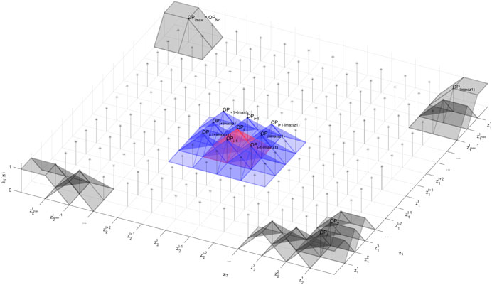
FIGURE 1. Illustrative example for pyramid-shaped membership functions $h_i(\underline{z})=h_i(z_1,z_2)$ with the two premise variables $\underline{z}={[z_1,z_2]}^T$ (formed by the triangular-shaped weighting functions w_1,l (z₁) and w_2,l (z₂), which are discretised in l (z_k)∈[1, l_max (z_k)] linearisation points; see Eq. 2 and exemplary visualisation of the $\text{eight}$ direct adjacent steady Operating Points (and linearisation points, respectively) $O{P}_{i-1-l_{\max }(z_1)}$ to $O{P}_{i+1+l_{\max }(z_1)}$ adjoining $O{P}_i$ with their membership functions (see the overlapping parts of the nine coloured pyramids) $h_{i-1-l_{\max }(z_1)}(z_1^{l-1},z_2^{l-1})$ to $h_{i+1+l_{\max }(z_1)}(z_1^{l+1},z_2^{l+1})$ (with $h_i(\underline{z})\ge 0$ within $z_1^{l-2}\le z_1\le z_1^{l+2}$ and $z_2^{l-2}\le z_2\le z_2^{l+2}$ for each of the nine steady operating points, while $h_i(\underline{z})=0$ holds for all the other steady operation points and $\underline{z}$, respectively; with i =(l (z₂)−1)l_max (z₁)+ l (z₁))

The weighting functions w_k,l (z_k) are combined to form the $(i_{\max }\equiv )Nr={\prod }_{k=1}^{k_{\max }}{l}_{\max }(z_k)$ membership functions $h_i(\underline{z})$ (with i ∈ [1, Nr]):

${\displaystyle \sum _{i=1}^{Nr}}{h}_i\left(\underline{z}\left(t\right)\right)={\displaystyle \prod _{k=1}^{k_{\max }}}{\displaystyle \sum _{l=1}^{l_{\max }\left(z_k\right)}}{w}_{k,l}\left(z_k\right).(3)$

In this contribution, the membership functions $h_i(\underline{z})$ just blend the i submodels, which are direct adjacent to the actual operation point (with $h_i(\underline{z})\ne 0$), while the membership functions of all other models are set to zero (i.e., $h_i(\underline{z})=0$), as described in e.g., (Pöschke et al., 2020) and illustrated in Figure 1.

In WT application, it is advantageous to define the reconstructed wind speed $\widehat{v}$ as the premise variable $\underline{z}\equiv \widehat{v}$.

Within this contribution individual input-matrices B_i, e.g., depending on the wind speeds v and rotor rotation speed ω_R, and a common output-matrix C_i ≡C, just describing the measurable states $\underline{y}$, are supposed.

2.1.2 Parallel-Distributed-Compensation-Controller With Feedforward Actuation

In the TS framework, a state-space controller $\underline{u}=-K\underline{x}$ with convexly blended state-feedback gains K_j—so-called Parallel Distributed Compensation (PDC) Controller (Wang et al. (1995), Tanaka and Wang (1997))—is usually used:

$\underline{u}=-{\displaystyle \sum _j^{Nr}}{h}_j\left(\underline{z}\right)K_j\left(\underline{x}-{\underline{x}}_{c,j}\right).(4)$

In Eq. 4 and the following, it is assumed, that $\underline{\widehat{z}}\to \underline{z}$ holds (as explained in Section 2.4.4).

If the disturbance attenuation is realised with a feedforward actuation, the PDC controller (Eq. 4) is extended to

$\underline{u}=\underset{{\underline{u}}_{FB}}{\underbrace{-{\displaystyle \sum _j^{Nr}}{h}_j\left(\underline{z}\right)K_j\left(\underline{x}-{\underline{x}}_{c,j}\right)}}+\underset{{\underline{u}}_{FF}}{\underbrace{{\displaystyle \sum _j^{Nr}}{h}_j\left(\underline{z}\right){\underline{u}}_{c,j}}}=-{\displaystyle \sum _j^{Nr}}{h}_j\left(\underline{z}\right)\left(K_j\left(\underline{x}-{\underline{x}}_{c,j}\right)-{\underline{u}}_{c,j}\right).(5)$

With the feedforward signal ${\underline{u}}_{FF}$ the disturbance is attenuated, while the feedback signal ${\underline{u}}_{FB}$ compensates control errors resulting from design model uncertainties.With Eq. 5 and ${\sum }_i^{Nr}{h}_i(z)=1$ in Eq. 1 the closed-loop dynamics (for i individual input matrices B_i, see Section 2.1.1)¹ is described by

$\begin{array}{ll}\hfill \underline{\dot{x}}& ={\displaystyle \sum _i^{Nr}}{h}_i\left(\underline{z}\right)\left(A_i\left(\underline{x}-{\underline{x}}_{c,i}\right)+B_i\left(\left(-{\displaystyle \sum _j^{Nr}}{h}_j\left(\underline{z}\right)\left(K_j\left(\underline{x}-{\underline{x}}_{c,j}\right)-{\underline{u}}_{c,j}\right)\right)-{\underline{u}}_{c,i}\right)\right)={\displaystyle \sum _i^{Nr}}{\displaystyle \sum _j^{Nr}}{h}_i\left(\underline{z}\right)h_j\left(\underline{z}\right)\left(A_i-B_i{K}_j\right)\left(\underline{x}-{\underline{x}}_{c,i}\right).\hfill \end{array}(6)$

2.1.3 Takagi-Sugeno Observer

For nonlinear systems $\dot{\underline{x}}=f(\underline{x},\underline{u})$ a weighted combination of linear Luenberger observers (Luenberge, (1971), Luenberger (1964)) can be used, which is denoted as Takagi-Sugeno Observer (TSO). The TS observer is obtained from the TS system Eq. 1 by introducing the output error-feedback term $L_i(\underline{y}-\underline{\widehat{y}})$ (Tanaka and Sano, 1994a). For a common output matrix C_i≡C (see Section 2.1.1) it holds²:

$\begin{array}{ll}\hfill \dot{\widehat{\underline{x}}}& ={\displaystyle \sum _i^{N_r}}{h}_i\left(\underline{z}\right)\left(A_i\left(\widehat{\underline{x}}-{\underline{x}}_{c,i}\right)+B_i\left(\underline{u}-{\underline{u}}_{c,i}\right)\right)+\left.{\displaystyle \sum _i^{Nr}}{h}_i\left(\underline{z}\right)\left(L_i\left(\underline{y}-\widehat{\underline{y}}\right)\right)\right|\widehat{\underline{y}}=C\widehat{\underline{x}}\hfill \\ \hfill & ={\displaystyle \sum _i^{N_r}}{h}_i\left(\underline{z}\right)\left(A_i\left(\widehat{\underline{x}}-{\underline{x}}_{c,i}\right)+B_i\left(\underline{u}-{\underline{u}}_{c,i}\right)+L_{i}C\left(\underline{x}-\widehat{\underline{x}}\right)\right)\hfill \end{array}(7)$

with the reconstructed states $\widehat{\underline{x}}$, the reconstructed outputs $\widehat{\underline{y}}$ and the error-feedback gains L_i.

For the error dynamics $\underline{\dot{e}}$

$\underline{e}≔\underline{x}-\underline{\widehat{x}}\Rightarrow \underline{\dot{e}}=\underline{\dot{x}}-\underline{\dot{\widehat{x}}}(8)$

it follows with Eqs 7, 1 in Eq. 8 (with the common output matrix C, see Section 2.1.1 and Section 2.2.2)²:

$\dot{\underline{e}}={\displaystyle \sum _i^{N_r}}{h}_i\left(\underline{z}\right)\left(A_i\left(\underline{x}-\underline{\widehat{x}}\right)+L_{i}C\left(\underline{x}-\widehat{\underline{x}}\right)\right)={\displaystyle \sum _i^{N_r}}{h}_i\left(\underline{z}\right)\left(A_i+L_{i}C\right)\underset{\underline{e}}{\underbrace{\left(\underline{x}-\widehat{\underline{x}}\right)}}.(9)$

Within this contribution (and the previously published works in (Gauterin et al., 2014) and (Pöschke et al., 2020)) the TS-observer is implemented to reconstruct the disturbing wind speed $\widehat{v}$, that is used as the premise variable $\underline{z}$, scheduling the feedforward and feedback signal (see Eq. 5 and Figure 3 with $\underline{z}=\widehat{v}$). Therefore, the TS-observer does not represent a typical disturbance observer for explicit disturbance rejection, rather than a premise observer to reconstruct the disturbance signal $\widehat{v}$ as premise variable $\underline{z}$, that is used to influence the controllable system inputs with the premise variable governed control signal scheduling (see explanation for Eq. 5 and Section 2.4.3). For the wind turbine application, the premise variable $\underline{z}$ often comprises the reconstructed, disturbing wind speed $\widehat{v}$ (within this contribution, the premise variable consists just of the reconstructed wind speed $\widehat{v}$, i.e. $\underline{z}=\widehat{v}$ holds), therefore the premise observer is also denoted as disturbance observer in the following (see also the observer classification in Section 2.4.3).

2.2 Global Lyapunov Approach Based Takagi-Sugeno Controller and Observer Design

The state-feedback gains K_j and error-feedback gains L_i are achieved from the stability condition, based on a Lyapunov approach: Assigning a simple, quadratic Lyapunov function, the following global stability condition yields

$\begin{array}{ll}\hfill V≔& {\underline{\mathcal{X}}}^{T}P\underline{\mathcal{X}}>0\hfill \\ \hfill \iff \dot{V}=& {\underline{\dot{\mathcal{X}}}}^{T}P\underline{\mathcal{X}}+{\underline{\mathcal{X}}}^{T}P\underline{\dot{\mathcal{X}}}<0\text{with}{P}^T=P\succ 0\hfill \end{array}(10)$

for the common and global, respectively, symmetric, positive definite matrix P ≻ 0 and the system-states $(\underline{\mathcal{X}},\dot{\underline{\mathcal{X}}})\equiv (\underline{x},\underline{\dot{x}})$ or error-states $(\underline{\mathcal{X}},\dot{\underline{\mathcal{X}}})\equiv (\underline{e},\underline{\dot{e}})$. That is, if the common, symmetric and positive definite matrix P exists, which holds the stability condition for the common and global, respectively, quadratic Lyapunov function V Eq. 10, the system is globally asymptotically stable and the state- and error-feedback-gain K_j and L_i can be derived from P as shown in the following two Subsection 2.2.1 and Subsection 2.2.2, further information given e.g., in (Lendek et al., 2010), (Wang et al., 1996) and (Tanaka and Sugeno, 1992).

Hereinafter, the Lyapunov approach Eq. 10 is denoted as the global Lyapunov approach.

2.2.1 Global Controller

LMI derivation

With Eq. 6 in Eq. 10 $(\underline{x}\equiv \underline{\mathcal{X}})$ it follows (for the individual input-matrices B_i)¹:

$\dot{V}={\underline{x}}^T\left({\displaystyle \sum _i^{Nr}}{\displaystyle \sum _j^{Nr}}{h}_i{h}_j\left(A_i^{T}P-K_j^T{B}_i^{T}P+P{A}_i-P{B}_i{K}_j\right)\right)\underline{x}<0.(11)$

With the pre- and postmultiplication P⁻¹ ⋅ □ and □⋅ P⁻¹, the thereby necessary substitution $X≔P^{-1}(\Rightarrow \stackrel{\mathrm{E}\mathrm{q}.\hspace{0.17em}10}{=}X)$ and the introduction of the slag parameter M_j = K_j X (to avoid the bilinear term K_j X within the resulting inequality) the following inequality for the Lyapunov function dynamics is derived from Eq. 11:

$\dot{V}={\underline{x}}^T\left({\displaystyle \sum _i^{Nr}}{\displaystyle \sum _j^{Nr}}{h}_i{h}_j\left(X{A}_i^T-M_j^T{B}_i^T+A_{i}X-B_i{M}_j\right)\right)\underline{x}<0.(12)$

The inequality Eq. 12 is solvable with a LMI-solver, if a discrete number of LMIs is derived from Eq. 12. Therefore, the convex properties of the membership functions h_i h_j are exploited to derive the following LMI set with the intended discrete number of LMIs:

$X{A}_i^T-M_j^T{B}_i^T+A_{i}X-B_i{M}_j\prec 0.(13)$

If the LMI set Eq. 13 is solvable, i.e., a positive definite matrix $X\left(=P^{-1}\right.$ with P ≻ 0, see Eq. 10) exists, the Lyapunov approach Eq. 10 (and its derivative Eq. 12) is fulfilled and the closed-loop system’s stability is guaranteed.

Controller design procedure

Once a common matrix P and the slag parameter M_j are found with the LMI solver, the state-feedback gains K_j are defined by K_j = M_j P. That is, for individual input matrices B_i the state-feedback gain K_j of the jth submodel and subcontroller, respectively, is designed in a way, that the subcontroller holds the LMI Eq. 10 and LMI set Eq. 13, the latter combining¹ the closed-loop dynamic of the jth submodel with the dynamic of all other or the direct adjacent submodels.

Number of LMIs

For the discrete number of combined¹ LMIs in the LMI set Eq. 13 it holds: $n_{\mathit{global,all}}^{\mathit{LMI,Cntrl}}=j_{\max }{i}_{\max }=N{r}^2$ (with i_max = j_max = Nr). This number can be reduced to $n_{\mathit{global,adj.}}^{\mathit{LMI,Cntrl}}<n_{\mathit{global,all}}^{\mathit{LMI,Cntrl}}$, if just submodels, that are direct adjacent to the jth submodel (see Section 2.1.1), are blended. Additionally, the stability condition Eq. 10 comprises a single LMI. That is, for the controller design with individual input matrices B_i the total LMI set consists of $n_{\mathit{global,all∕adj.}}^{\mathit{LMI,Cntrl}}+1$ LMIs. For the global Lyapunov approach with the global and single P-matrix, respectively this total LMI set is solved with a single execution of the LMI solver, i.e., the $n_{\mathit{global,all\; /\; adj.}}^{\mathit{LMI,Cntrl}}+1$ LMIs are solved simultaneously.

2.2.2 Global Observer

LMI derivation

With Eq. 9 in Eq. 13 $(\underline{e}\equiv \underline{\mathcal{X}})$ it follows (for the common output-matrix C_i ≡ C)²:

$\dot{V}={\underline{e}}^T\left({\displaystyle \sum _i^{Nr}}{h}_i\left(A_i^{T}P-C^T{L}_i^{T}P+P{A}_i-P{L}_{i}C\right)\right)\underline{e}<0.(14)$

With the introduction of the slag parameter N_i = P L_i (to avoid the bilinear term P L_i within the resulting inequality) the following inequality for the error dynamics is derived from Eq. 14:

$\dot{V}={\underline{e}}^T\left({\displaystyle \sum _i^{Nr}}{h}_i\left(A_i^{T}P-C^T{N}_i^T+P{A}_i-N_{i}C\right)\right)\underline{e}<0.(15)$

Eq. 15 holds (as explained for Eq. 12), if the LMI set

$A_i^{T}P-C^T{N}_i^T+P{A}_i-N_{i}C\prec 0(16)$

is satisfied, i.e., a positive definite matrix P ≻ 0 (see Eq. 10) exists, so that the Lyapunov approach Eq. 10 (and its derivative Eq. 15) is fulfilled and the error system’s stability is guaranteed.

Observer design procedure

Once a common matrix P and the slag parameter N_i are found with the LMI solver, the error-feedback gains L_i are defined by L_i = P⁻¹ N_i. That is, for a common output matrix C_i ≡ C the error-feedback gain L_i of the ith submodel and subobserver, respectively is designed in a way, that the subobserver holds the LMI Eq. 10 and the LMI set Eq. 16, the latter just comprising the error dynamics of each single submodel (A_i, B_i) in an individual and single LMI, respectively (and not combining the dynamics of all or direct adjacent submodels).

Number of LMIs

For the discrete number of individual LMIs in the LMI set Eq. 16 it holds: $n_{\mathit{global}}^{\mathit{LMI,Obs}}=i_{\max }=Nr$. As Eq. 16 defines a single LMI for each submodel and subobserver, respectively, there is no need to consider direct adjacent submodels in the observer design with a common output matrix C. Additionally, the stability condition Eq. 10 comprises a single LMI. That is, for the observer design with a common output matrix C the total LMI set consists of $n_{\mathit{global}}^{\mathit{LMI,Obs}}+1$ LMIs. For the global Lyapunov approach with the global and single P-matrix, respectively this total LMI set is solved with a single execution of the LMI solver. i.e., the $n_{\mathit{global}}^{\mathit{LMI,Obs}}+1$ LMIs are solved simultaneously.

2.3 Local Lyapunov Approach for Takagi-Sugeno Controller and Observer Design

For the proposed local Lyapunov approach the local stability condition

$\begin{array}{ll}\hfill V_i≔& {\underline{\mathcal{X}}}^T{P}_i\underline{\mathcal{X}}>0\hfill \\ \hfill \iff \dot{V_i}=& {\underline{\dot{\mathcal{X}}}}^T{P}_i\underline{\mathcal{X}}+{\underline{\mathcal{X}}}^T{P}_i\underline{\dot{\mathcal{X}}}<0\text{with}{P}_i^T=P_i\succ 0\text{and}i\in \left[1,Nr\right]\hfill \end{array}(17)$

holds for the individual and local, respectively, symmetric, positive definite matrix P_i ≻ 0 and the system-states $(\underline{\mathcal{X}},\dot{\underline{\mathcal{X}}})\equiv (\underline{x},\underline{\dot{x}})$ or error-states $(\underline{\mathcal{X}},\dot{\underline{\mathcal{X}}})\equiv (\underline{e},\underline{\dot{e}})$. Compared to the common and global Lyapunov-approach Eq. 10, a number of Nr individual Lyapunov functions V_i (with i ∈ [1, Nr]) are used instead of one common Lyapunov function V (in the global Lyapunov approach Eq. 10). That is, for each submodel (A_i, B_i) an individual Lyapunov function V_i is defined.

Accordingly, the LMI derived for the closed-loop dynamics Eq. 13 and error dynamics Eq. 16 is simplified, as the convex blending becomes obsolete, if the Lyapunov stability condition is defined for each submodel individually (compare Eq. 18 with Eq. 12 and Eq. 20 with Eq. 15).

2.3.1 Local Controller LMI

For the local Lyapunov approach the inequality derived for the closed-loop dynamics (with $(\underline{\mathcal{X}},\dot{\underline{\mathcal{X}}})\equiv (\underline{x},\underline{\dot{x}})$) results in

$\begin{array}{ll}\hfill \dot{V}& ={\underline{x}}^T\left(X_i{A}_i^T-M_i^T{B}_i^T+A_i{X}_i-B_i{M}_i\right)\underline{x}<0\hfill \\ \hfill \text{with}{X}_i& ≔P_i^{-1}\text{and}{M}_i=K_i{X}_i.\hfill \end{array}(18)$

The inequality (Eq. 18) holds, if the LMI

$X_i{A}_i^T-M_i^T{B}_i^T+A_i{X}_i-B_i{M}_i\prec 0(19)$

is satisfied, i.e., individual and local, respectively positive definite matrices X_i exist, which fulfill Eq. 19.

2.3.2 Local Observer LMI

The same simplification holds for the error dynamics, i.e. for the local Lyapunov approach the inequality derived for the error dynamics (with $(\underline{\mathcal{X}},\dot{\underline{\mathcal{X}}})\equiv (\underline{e},\underline{\dot{e}})$) results in:

$\begin{array}{ll}\hfill \dot{V}& ={\underline{e}}^T\left(A_i^T{P}_i-C^T{N}_i^T+P_i{A}_i-N_{i}C\right)\underline{e}<0\hfill \\ \hfill \text{with}{N}_i& =P_i{L}_i.\hfill \end{array}(20)$

The inequality (Eq. 20) holds, if the LMI

$A_i^T{P}_i-C^T{N}_i^T+P_i{A}_i-N_{i}C\prec 0(21)$

is satisfied, i.e. individual and local, respectively positive definite matrices P_i exist, which fulfill Eq. 21.

2.3.3 Local Controller and Observer Design Procedure

Once the individual matrix P_i and the slag parameter M_i (for local controller design) or N_i (for local observer design) is found with the LMI solver, the state-feedback gain K_i or error-feedback gain L_i is defined by K_i = M_i P_i or $L_i=P_i^{-1}{N}_i$. That is, the state-feedback gain K_i or error-feedback gain L_i of the ith submodel and subcontroller or subobserver, respectively is designed in a way, that the subcontroller or subobserver holds the LMI Eq. 17 and the LMI set Eq. 19 or Eq. 21, the latter just comprising the state or error dynamics of each single submodel (A_i, B_i) in an individual and single LMI, respectively (and not combining the dynamics of all or direct adjacent submodels).

2.3.4 Number of LMIs

As the local Lyapunov approach simplifies and reduces, respectively the set of combined LMIs (for the local Lyapunov approach the LMI set comprises just two LMIs: LMI Eq. 19 or Eq. 21 and the LMI of the positive definite matrix P_i ≻ 0, see Eq. 17), the parallel and simultaneously, respectively to be solved LMIs are reduced (from $n_{\mathit{global,all∕adj.}}^{\mathit{LMI,Cntrl}}+1>n_{\mathit{global}}^{\mathit{LMI,Obs}}(=Nr+1)$ to $n_{\mathit{Local}}^{\mathit{LMI,Cntrl∕Obs}}=2$ LMIs), too. Thereby, the LMI solver is executed Nr times consecutively for the local Lyapunov approach (due to the individual P_i-matrix in Eq. 17), while the LMI solver for the global Lyapunov approach is executed just once, because of the common P matrix in Eq. 10. Therefore, the flexibility of the LMI solver in assigning desired pole locations of the closed-loop system is increased for the local Lyapunov approach. The less conservative task for the LMI solver enables the specification of tighter performance constraints for the local Lyapunov approach, e.g., smaller pole regions (by implementing pole region constraints in form of additional LMIs, see Section 2.5), and results in more flexible and consistent specifications of the desired closed-loop dynamics, denoted as the general objective of the local Lyapunov approach.

2.3.5 Subsequent, Global Lyapunov Stability Analysis

Note: With the local Lyapunov approach and the resulting LMIs Eq. 19 and Eq. 21, just the small signal stability is evaluated, i.e., considering the operating point depicted in the linear submodel, if a positive definite matrix P_i exists. To ensure the global stability of the convexly blended submodels, a final stability analysis has to be performed, enveloping all combined closed-loop submodels. This final stability analysis is executed in the subsequent, global Lyapunov stability analysis described in Section 2.4.4.

2.4 Local Lyapunov Approach in Wind Turbine Control Application

2.4.1 Structural Dynamical Design Model

For the wind turbine (WT) controller design, the authors use simplified structural dynamical models, based on lumped-masses and joined with discrete spring- and damper-elements (e.g., (Bianchi et al., 2007), (Georg, 2015) or (Pöschke et al., 2020)). These models comprise just the essential and costly wind turbine components rotor, drive train and tower. Within this contribution, the rotor blade dynamic is represented, while the tower dynamic is neglected (see Figure 2). The rotor model is composed of the rotor $\mathcal{B}$lades, rotating as one rigid body in the rotor plane (denoted with rotor rotation (speed) ${\omega }_{\mathcal{R}}$ in Figure 2) and translating with $x_{\mathcal{B}}$ in and against the wind direction (denoted by the subscripted index $\mathcal{B}$). The drive train is represented by its rigid body Rotation (denoted by the subscripted index $\mathcal{R}$).

FIGURE 2

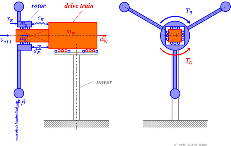
FIGURE 2. Structural dynamical design model of a wind turbine (in side- and front-view) with the two degree of freedom: • $\text{blade translation}{x}_{\mathcal{B}}$ (in up- and downwind direction) and • drive train dynamic, i.e., $\text{rotor and generator rotation (speed)}{\omega }_{\mathcal{R}}$ for the rigid body model of the rotor and drive train. The blue depicted ball bearings enable just the translation $x_{\mathcal{B}}$ of the discrete rotor model in relation to the discrete drive train model (i.e., in wind direction), while the red depicted bearings enable just the drive train rotation ${\omega }_{\mathcal{R}}$ along its horizontal axis and suspend any other coupling of drive train rotation and tower translation. Linear, single headed arrows represent translations, forces or translatory spring- and damper-elements, while linear, double headed arrows represent rotations. The parameters $m_{\mathcal{K}}$, $c_{\mathcal{K}}$ and $d_{\mathcal{K}}$ represent the discrete component masses, discrete spring coefficients and discrete damping coefficients of the discrete component model $\mathcal{K}$ (with $\mathcal{K}=\mathcal{B}$(lade) or $\mathcal{K}=\mathcal{R}$(otation) of the drive train.)

After linearising an elaborated WT simulation model for i stationary operating points OP_i (with i ∈ [1, Nr]), the controller design submodels $(A_{i\mathcal{B}/\mathcal{R}},B_{i\mathcal{B}/\mathcal{R}})$ are composed with the linearisation coefficients. Thereby, mechanical couplings between those components are specified or neglected, as explained in Section 2.4.4. The specification of the design submodels $(A_{i\mathcal{B}/\mathcal{R}},B_{i\mathcal{B}/\mathcal{R}})$ are given in Tables A2, A3 in the appendix.

2.4.2 Wind Turbine Control Objectives, Loading and Operation Concept

In wind turbine (WT) application the controller intends—besides energy yield optimisation—for mechanical load mitigation, due to vast environmental loads acting on the complete WT structure. Besides the ultimate, mechanical loads (that occur for single moments and the corresponding ultimate stress must not exceed the material strength), fatigue, mechanical loads have to be examined. Those fatigue loads, also denoted as Damage Equivalent Loads (DEL, i.e., a mean amplitude with the equivalent damaging effect like constantly or stochastically changing amplitudes, e.g., resulting from turbulent wind time series), characterise the damaging effect resulting from load cycles, occurring all over the components’ lifetime (Clem ens et al., 2020).

Ascribed to the generator characteristics, two operating modes have to be distinguished: In the partial load range, the generator is operated below rated power and the energy yield is optimised by generator torque T_G control, i.e., the generator torque T_G is one of the two actuating signals. In full load range, the generator is operated at rated power. Therefore, the energy extraction from the inflow with the WT rotor is restricted to rated generator power by the pitch angle β control, influencing the blade aerodynamics and mechanical torque T_R generation of the rotor by rotating the complete rotor blade along its longitudinal axis (see Figure 2). Hence, the pitch angle β is the second actuating signal of a wind turbine controller, i.e., $\underline{u}={[\beta ,T_G]}^T$ holds. In this contribution, a collective pitch control algorithm is utilised, i.e., all blades are actuated with the same pitch angle. In Appendix Table A1, the control signals ${\underline{u}}_{c,i}={[{\beta }_{c,i},T_{G,c,i}]}^T$ for all 27 stationary operating points in partial and full load range are listed.

2.4.3 Implemented Wind Turbine Controller Structure

Within this contribution an observer-based feedforward-feedback controller in TS framework is utilised and applied to wind turbine control.

For the feedforward-feedback controller the extended parallel distributed compensation (PDC) controller Eq. 5 is used.

To attenuate the effect of the disturbing wind speed, a disturbance-observer is used (see Section 2.1.3 and Figure 3) to determine the rotor effective wind speed v_eff. For the disturbance observer, the WT main component model (see Section 2.4.1 and Section 2.4.4) with the highest disturbance sensitivity is used, i.e., for wind turbine systems the downwind and upwind blade deflection $x_{\mathcal{B}}$³ is most sensitive to disturbances caused by wind speed fluctuations, due to the very low bending stiffness of the blades (in normal direction to its profile chord). Therefore, the disturbance observer reconstructs the disturbing, effective wind speed $\widehat{v}\equiv v_{\mathit{eff}}$ and blade translation speed ${\dot{\widehat{x}}}_{\mathcal{B}}$ from the blade translation error $e_{x_{\mathcal{B}}}$ determined from the measured and reconstructed blade translation $e_{x_{\mathcal{B}}}=x_{\mathcal{B}}-{\widehat{x}}_{\mathcal{B}}$. For this purpose, the disturbance observer design model is augmented by a simple wind model (Ekelund, 1994), expanding the state vector ${\underline{\widehat{x}}}_{\mathcal{B}}$ with the reconstructed wind speed $\widehat{v}$ (and disturbance signal $\underline{d}\equiv \widehat{v}$, respectively) ${\underline{\widehat{\tilde{x}}}}_{\mathcal{B}}={[{\underline{\widehat{x}}}_{\mathcal{B}},\widehat{v}]}^T$ and augmenting the state space model Eq. 7 and Eq. 9 accordingly (with ${\tilde{A}}_i,{\tilde{B}}_i$ and $\tilde{C}$; see also (Pöschke et al., 2020)). Therefore, the used TS disturbance observer, resulting from the integration of a disturbing model in the plant model and augmenting the state vector ${\underline{\widehat{x}}}_{\mathcal{B}}$ with the disturbing wind state $\widehat{v}$, is classified as an Extended State Observer (see (Li et al., 2014)), that is represented in the Takagi-Sugeno framework.

FIGURE 3

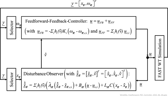
FIGURE 3. Block digram of the observer-based Takagi-Sugeno wind turbine controller.

The reconstructed wind speed $\widehat{v}$ is defined as premise variable $\underline{z}$, scheduling the nonlinearity of the system and utilised for the membership function $h_i(\underline{z})$ of the feedforward signal ${\underline{u}}_{FF}$ and feedback signal ${\underline{u}}_{FB}$ in Eq. 5. Therefore, the disturbance observer does not intend for a disturbance rejection, rather than for an observer-based controller scheme with disturbance reconstruction, influencing the controllable system inputs (see also Section 2.1.3).

Within this contribution, triangular-shaped⁴ membership functions h_i(z) are used, just blending directly adjacent submodels (A_i, B_i) (see Figure 1 and the explanations in Section 2.1.1). Because of the reduced number of (triangular) membership functions (i.e., just the direct adjacent membership functions are taken into account and not all membership functions), also the number of submodels included in the feedback controller and observer design—based on the global Lyapunov approach—is reduced (see Section 2.3) (Note: For the local Lyapunov approach an individual Lyapunov function V_i is defined for each submodel (A_i, B_i), because of the local stability condition Eq. 17. Therefore, the convex blending with the membership functions $h_i(\underline{z})$ is obsolete and the form of the membership functions has no influence on the design, as just the i th submodel is included in the observer design—see Section 2.3.)

The augmented state, input and output matrices ${\tilde{A}}_i,{\tilde{B}}_i$ and $\tilde{C}$, as well as the augmented steady system states ${\underline{\tilde{x}}}_{c,i}$ and steady input states ${\underline{u}}_{c,i}$, used within this contribution, are given in Table A2 to Table A6. Additionally, the state feedback gain matrices K_i and error-feedback gain matrices $L_{i\mathcal{B}}^w$ are listed in Table A7 and Table A8.

2.4.4 Decomposed Wind Turbine System and Subsequent Lyapunov Stability Analysis

Mechanical and mechatronic systems, like wind turbines (WT), are characterised by the pole locations of the coupled mechanical components. Due to the widely spaced, open-loop pole locations of the WT system (see Figure 4 and Section 4), it is advantageous for the controller and observer design models to decompose the coupled, nonlinear system submodel (A_i, B_i) into decoupled reduced submodels—denoted with component models—just comprising the dynamics of the individual, mechanical main components like the rotor blade submodels $(A_{i\mathcal{B}},B_{i\mathcal{B}})$ and drive train submodels $(A_{i\mathcal{R}},B_{i\mathcal{R}})$ (also described in (Pöschke et al., 2020), but now upgraded with the rotor blade submodels $(A_{i\mathcal{B}},B_{i\mathcal{B}})$).

FIGURE 4

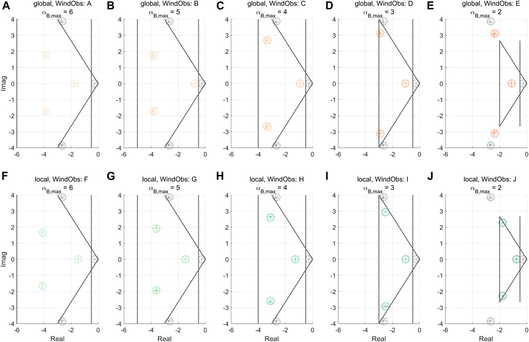
FIGURE 4. Pole locations of the error dynamics (achieved within the wind speed observer design) for an increasing upper bound ${\alpha }_{\mathcal{B},\max }$ (from left to right), applied to the $\text{global Lyapunov approach}$ (upper row) and $\text{local Lyapunov approach}$ (lower row), restricted to the four submodels i ∈[15,18] that are relevant for the wind turbine simulations with the prescribed wind speeds v(t) between 14 m/s and 16 m/s. The Open-Loop, real-valued poles $s_{P,i}^{OL,p}$ (with p = 1) of the wind model and the open-loop, conjugate complex-valued poles of the blade model $s_{P,i}^{OL,p}$ (with p = 2 ∨ p = 3) are depicted in grey colour, while the closed-loop real-valued (p = 1, see Section 3.2 and Table 2) and closed-loop, conjugate complex-valued (p = 2 ∨ p = 3) poles $s_{P,i}^{w,p}$ of the $\text{global wind observers}(\text{with}\hspace{0.17em}w\in [A,\hspace{0.17em}E])$ and the $\text{local wind observers}(\text{with}\hspace{0.17em}w\in [F,\hspace{0.17em}J])$ are depicted in green or orange colour and are distinguished by the superscripted index w.

Thereby, couplings between the components’ degree of freedom are neglected within the component controller and observer design models, like the missing axial coupling between drive train and main frame/tower depicted in Figure 2 (just plain ball bearings are defined). Despite this substantial assumption, the component design models achieve satisfying controller performance, while increasing the controller design flexibility significantly.

The corresponding design models are derived from the elaborated NREL FAST 5 MW reference wind turbine (Jonkman, 2016; Jonkman and Buhl (2005) and Jonkman et al. (2009)) simulation model, based on a convex sum of 27 linearised submodels (defined for piecewise equidistant, steady and effective wind speeds from v ∈ [3 m/s, 25 m/s]; see Table A1), received from the NREL FAST WT linearisation (Jonkman and Jonkman, 2016). Within this linearisation, all aerodynamic and structural dynamic characteristics defined in the elaborated NREL FAST 5 MW reference wind turbine are accounted (see also explanations given in (Pöschke et al., 2020)).

Once the component controllers and observers are designed, the corresponding state-feedback gains ($K_{i\mathcal{R}}$, $K_{i\mathcal{B}}$) and observer gains $\left(L_{i\mathcal{R}}\right.$, $L_{i\mathcal{B}}$) are superposed for the overall controller gain K_i and observer gain L_i. The stability of the convexly blended i submodels is analysed with the superposed gains K_i and L_i in a subsequent, global Lyapunov stability analysis (see Section 2.3.5), separately for the controller and error dynamics (Yoneyama et al. (1998), Ma et al. (1998)). Although, the separation principle and overall stability proof, respectively of separately designed observer and controller is just valid for measurable premise variables $\underline{z}$ (Yoneyama et al. (1998), Ma et al. (1998)), it is shown in (Pöschke et al., 2022) for a separated observer and controller design, that the overall stability is also ensured for reconstructed premise variables $\underline{\widehat{z}}$, under the assumption of a maximum estimation error in the premise variable with $\underline{\widehat{z}}\to \underline{z}$. Therefore, the stability proof and separation principle, respectively holds for $\underline{\widehat{z}}\to \underline{z}$. Even though the maximum error estimation is missing in this contribution, it is assumed, that $\underline{\widehat{z}}\to \underline{z}$ and the separation principle holds. The missing error estimation and overall stability proof corresponding to (Pöschke et al., 2022) has to be given in future work. That is, within this contribution just separated controller and observer syntheses are executed in regard to a pragmatic design process that intends for less conservative state and error state feedback gains K_i and L_i, like explained in Section 1. Thus, the design process is focused on an automated controller and observer design, i.e., the Lyapunov approach was selected to achieve the controller and observer gains in a systematic and traceable procedure, rather than to ensure the overall stability of the observer-based system dynamics. Though, the stability condition of the Lyapunov approach is exploited (separately in the controller and observer design) to abbreviate the iterative design process, i. e., all controller and observer design parameter specifications, resulting in unstable dynamics, are eliminated within the controller and observer synthesis to expedite the design process.

2.5 LMI Constraints of the Pole Regions

With the linear matrix inequalities Eqs 13, 16, 19 and Eq 21 the pole locations are just restricted to the left half of the complex pole map. Additional constraints need to be defined to tighten the pole location on smaller pole regions. As described in (Chilali and Pascal, 1996), additional bounds specified in the complex pole map can be transformed into LMI, which are applied to wind turbine control e.g., in (Pöschke et al., 2019). Within this contribution, just vertical upper and lower bounds (representing the maximum and minimum decay rate ${\alpha }_{\mathcal{B},\max }$ and ${\alpha }_{\mathcal{B},\min }$) and a cone angle θ (representing the Damping ratio D with D = cos(θ)) are used and described in the Appendix Section A1.3. With these constraints, pole regions with symmetrical trapezium shape are defined (see Figure 4).

3 Simulations and Results

With the local Lyapunov approach, the general objective of a more flexible specification of the pole locations and increased consistency in the desired and achieved closed-loop system dynamics is intended (see Section 2.3.4). This general objective is analysed within this contribution for a wind turbine specific, particular objective—the decreased observer performance and feedforward actuation—described in Section 3.1. The achieved results from wind turbine simulations are presented in Section 3.2.

3.1 Simulation Design: Particular Objective of the Local Lyapunov Approach Within this Contribution

Within this contribution, the general objective of the local Lyapunov approach (see Section 2.3.4) is assessed for a particular wind speed observer performance, hereinafter denoted with the particular objective, supposed to be beneficial regarding load mitigation: For turbulent wind excitation, high mechanical loads (especially fatigue loads) often result from brisk feedforward actuation⁵. Therefore, the proposed local Lyapunov approach shall yield for a decreased disturbance reconstruction $\widehat{v}$ performance—affecting the premise variable $\widehat{v}$—to attenuate the premise variable $\widehat{v}$ driven feedforward actuation ${\underline{u}}_{FF}(h_i(\widehat{v}))$ (see Eq. 5) with $\underline{z}\equiv \widehat{v}$) and to increase the feedback compensation ${\underline{u}}_{FB}(h_i(\widehat{v}))$ (see Section 2.1.2). That is for this particular objective, the closed-loop dynamics is defined in such a way, that the performance of the wind speed $\widehat{v}$ reconstruction and the precision of the feedforward actuation ${\underline{u}}_{FF}(h_i(\widehat{v}))$ is intentionally lowered to achieve rising deviations, which are compensated by increased feedback controller actuation ${\underline{u}}_{FB}(h_i(\widehat{v}))$. As the error-feedback gains L_i govern the observer performance and these gains are achieved from the observer design according to the specified error-feedback pole regions, the pole region specification is varied by shrinking its size. That is, a significant modification of the pole regions is conducted with the local Lyapunov approach to achieve the particular objective of a decreased observer performance, resulting in mitigated mechanical loads, especially mitigated fatigue loads. To lower the wind speed observer performance and error dynamics (i.e., the wind speed $\widehat{v}$ depending error-feedback gains L_i in ${\sum }_i^{Nr}{h}_i(\widehat{v})L_{i}C\left(\underline{x}-\widehat{\underline{x}}\right)=L(\widehat{v})C\underline{e}$⁶), the upper bound ${\alpha }_{\mathcal{B},\max }$ of the error dynamics’ pole region is increased, i.e., shifted towards the imaginary axis in the left half of the complex pole map, while the lower bound ${\alpha }_{\mathcal{B},\min }$ (located close to the open-loop poles) is kept constant (see Figure 4). It is expected, that the error-feedback gains L_i decrease with increasing upper bounds ${\alpha }_{\mathcal{B},\max }$ $({\alpha }_{\mathcal{B},\max }\nearrow \Rightarrow L_i\searrow )$, as the distances between open-loop poles and closed-loop poles of the error dynamics $\mathrm{\Delta }{s}_{P,i}^{w,p}({\alpha }_{\mathcal{B},\max })$ decrease with increasing upper bounds ${\alpha }_{\mathcal{B},\max }$ and the quantity of the error-feedback gain depends on this distance $|L_i|=f(\mathrm{\Delta }{s}_{P,i}^{w,p})$⁷.

To distinguish the pole locations $s_P^w$ (see Figure 4), error-feedback gains $L_i^w$ (see Table A8) or mechanical loads like $S_{eq}^w$ (see Figure 8), resulting from a number of w different error-feedback pole region specifications, the superscript index w (denoting the w different error-feedback pole regions and corresponding wind speed observers) is introduced in the following. To analyse the error-feedback gains $L_{i\mathcal{B}}^w$ of the $\mathcal{B}$lade model-based wind speed observer, the following state space equation is relevant (see Eq. 7), describing the reconstructed blade component dynamics:

$\begin{array}{ll}\hfill \underset{\underline{\dot{\widehat{\stackrel{̃}{x}}}}}{\underbrace{\left[\begin{array}{c}\hfill {\dot{\widehat{x}}}_{\mathcal{B}}\hfill \\ \hfill {\ddot{\widehat{x}}}_{\mathcal{B}}\hfill \\ \hfill \dot{\widehat{v}}\hfill \end{array}\right]}}& ={\displaystyle \sum _i^{N_r}}{h}_i\left(\underline{z}\right)\left(A_i\left(\widehat{\underline{\tilde{x}}}-{\underline{\tilde{x}}}_{c,i}\right)+B_i\left(\underline{u}-{\underline{u}}_{c,i}\right)\right)+\hfill \\ \hfill & {\displaystyle \sum _i^{Nr}}{h}_i\left(\widehat{v}\right)\underset{L_{i\mathcal{B}}^w}{\underbrace{\left[\begin{array}{c}\hfill L_{i\mathcal{B}}^{w,1}\hfill \\ \hfill L_{i\mathcal{B}}^{w,2}\hfill \\ \hfill L_{i\mathcal{B}}^{w,3}\hfill \end{array}\right]}}\underset{C_{\mathcal{B}}}{\underbrace{\left[100\right]}}\underset{\underline{e}}{\underbrace{\left[\begin{array}{c}\hfill x_{\mathcal{B}}-{\widehat{x}}_{\mathcal{B}}\hfill \\ \hfill {\dot{x}}_{\mathcal{B}}-{\dot{\widehat{x}}}_{\mathcal{B}}\hfill \\ \hfill v-\widehat{v}\hfill \end{array}\right]}}\hfill \end{array}$

$\begin{array}{ll}\hfill & ={\displaystyle \sum _i^{N_r}}{h}_i\left(\underline{z}\right)\left(A_i\left(\widehat{\underline{\tilde{x}}}-{\underline{\tilde{x}}}_{c,i}\right)+B_i\left(\underline{u}-{\underline{u}}_{c,i}\right)\right)+\hfill \\ \hfill & {\displaystyle \sum _i^{Nr}}{h}_i\left(\widehat{v}\right)\left[\begin{array}{ccc}\hfill L_{i\mathcal{B}}^{w,1}\hfill & \hfill 0\hfill & \hfill 0\hfill \\ \hfill L_{i\mathcal{B}}^{w,2}\hfill & \hfill 0\hfill & \hfill 0\hfill \\ \hfill L_{i\mathcal{B}}^{w,3}\hfill & \hfill 0\hfill & \hfill 0\hfill \end{array}\right]\left[\begin{array}{c}\hfill x_{\mathcal{B}}-{\widehat{x}}_{\mathcal{B}}\hfill \\ \hfill {\dot{x}}_{\mathcal{B}}-{\dot{\widehat{x}}}_{\mathcal{B}}\hfill \\ \hfill v-\widehat{v}\hfill \end{array}\right]\hfill \end{array}(22)$

with the j components ${\dot{\widehat{\stackrel{̃}{x}}}}^j$ of the reconstructed and augmented state vector $\stackrel{̇}{\widehat{\underline{\tilde{x}}}}$ and with j matrix elements $L_{i\mathcal{B}}^{w,j}$ of the error-feedback gain $L_{i\mathcal{B}}^w$.

Within this contribution, the general objective of an increased flexibility in the observer-based controller design and increased consistency of the desired and achieved system dynamics (see Section 2.3.4) is analysed with the particular objective of an decreased observer performance and feedforward actuation, resulting from shrinking pole regions. That is, for both Lyapunov approaches identical upper bound variation and shrinking pole regions are defined and the flexibility and consistency of both approaches are compared with the help of several metrics (like pole locations, error-feedback gains, reconstructed wind speeds, pitch angles, pitch rate and rotation speed deviations): Regarding the flexibility, the minimum pole region dimension is determined. That is, for all poles it is examined, if the poles are located inside the imposed pole region after executing the error-feedback gain L_i design. The intended, particular objective of a decreased observer performance of the local Lyapunov approach is fulfilled, if this approach leads to a smaller, minimum pole region than the global Lyapunov approach, enabling the specification of tighter performance constraints for the system dynamics. Regarding the consistency of desired and achieved system dynamics, it is analysed, if the shrinking poles regions result in decreased feedforward pitch angles β_FF and increased feedback pitch angles β_FB with decreased pitch rates $\dot{\beta }$ and increased, resulting rotation speed deviations Δω.

In addition, the control objectives of mitigated ultimate and fatigue loads are analysed for identical WT controller pole region specifications, but related to both disturbance observer design approaches.

3.2 Simulation Results: Disturbance Observer Variation, Resulting System Dynamics and Mechanical Loads

For each Lyapunov approach, five different disturbance observers for the $\text{global Lyapunov approach}$ (denoted in the following with the superscripted index $\text{w}\text{in}\left[A,,,E\right])$ and for the $\text{local Lyapunov approach}$ (denoted with $w\in \left[F,,,J\right]$ are designed—based on five different pole regions with shrinking size—and the resulting closed-loop dynamics as well as the resulting mechanical loads on the WT components are analysed.

Pole regions and submodels

In Table 1, the pole region specifications for both design approaches are listed. For the analysed wind time series excitation with prescribed wind speeds v(t) between 14 m/s and 16 m/s, just four of the i ∈ [1,27], from linearisation achieved submodels (denoted with the subscripted index i) are convexly blended. Therefore, just these four submodels (A_i, B_i) with i ∈ [15,18] are taken into account in the results and discussion.

TABLE 1

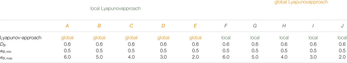
TABLE 1. Description of the TS disturbance observers (i.e., wind speed observers) (for the wind speed observers w in A to E, based on the $\text{global Lyapunov-approach}$ and for the wind observers w in F to J, based on the $\text{local Lyapunov-approach}$, with the cone angle, and the lower and the upper bounds of the five pole regions (see Figure 4), defined by the $\mathcal{B}$lade error state damping $D_{\mathcal{B}}$ and the $\mathcal{B}$lade decay rates ${\alpha }_{\mathcal{B},\min }$ and ${\alpha }_{\mathcal{B},\max }$).

Pole locations

Figure 4 shows the resulting p pole locations $s_{P,i}^{OL/w,p}$ of the corresponding open-loop dynamics (denoted with the superscripted index OL), as well as the closed-loop dynamics (denoted with the superscripted index w for the $\text{w} \text{in}\left[A,,,E\right])$ $\text{global}\text{wind speed observers}$ and $w\in \left[F,,,J\right]\text{local wind observers}$) and error dynamics, respectively, achieved within the disturbance observer design, in the complex pole map. As the disturbance observer design model and wind speed observer design model, respectively, consists of the vibrating $\mathcal{B}$lade model (with its two states ${\widehat{x}}_{\mathcal{B}},{\dot{\widehat{x}}}_{\mathcal{B}}$ see Eq. 22) and the non-vibrating wind model (with the wind speed state $\widehat{v}$), the design model posses three poles (i.e., p ∈ [1,3]): the conjugated-complex blade poles $s_{P,i}^{OL/w,2\vee 3}$ (inside the pole map, for p = 2 ∨ p = 3) and the real-valued wind model pole $s_{P,i}^{OL/w,1}$ (on the real axis of the pole map, for p = 1). In Table 2 the distances

$\mathrm{\Delta }{s}_{P,i}^{w,p}=\sqrt{{\left(\text{Re}\left(s_{P,i}^{OL,p}\right)-\text{Re}\left(s_{P,i}^{w,p}\right)\right)}^2+{\left(\text{Im}\left(s_{P,i}^{OL,p}\right)-\text{Im}\left(s_{P,i}^{w,p}\right)\right)}^2}(23)$

between open-loop poles $s_{P,i}^{OL,p}$ and closed-loop poles $s_{P,i}^{w,p}$ in the pole map are given for each of the p ∈ [1,3] poles of the wind and blade model. Additionally, the related average distance

$\mathrm{\Delta }{s}_{P,i}^{w,\bar{p}}=\frac{1}{3}{\displaystyle \sum _{p=1}^3}\mathrm{\Delta }{s}_{P,i}^{w,p}=\frac{1}{3}\left(\mathrm{\Delta }{s}_{P,i}^{w,1}+\mathrm{\Delta }{s}_{P,i}^{w,2}+\mathrm{\Delta }{s}_{P,i}^{w,3}\right)(24)$

of the single submodel i and the average distance

$\mathrm{\Delta }{s}_{P,\bar{i}}^{w,\bar{p}}=\frac{1}{4}{\displaystyle \sum _{i=15}^{18}}\mathrm{\Delta }{s}_{P,i}^{w,\bar{p}}=\frac{1}{4}\left(\mathrm{\Delta }{s}_{P,15}^{w,\bar{p}}+\mathrm{\Delta }{s}_{P,16}^{w,\bar{p}}+\mathrm{\Delta }{s}_{P,17}^{w,\bar{p}}+\mathrm{\Delta }{s}_{P,18}^{w,\bar{p}}\right)(25)$

of all four submodels are listed in Table 2.

TABLE 2

TABLE 2. Distances $\mathrm{\Delta }{s}_{P,i}^{w,p}$ between the open-loop pole location $s_{P,i}^{OL,p}$ and closed-loop pole locations $s_{P,i}^{w,p}$ of each of the p ∈ [1,3] poles (with p = 1 for the real-valued pole of the wind model and p = 2,3 for the complex-valued poles of the blade model) of a single submodel i in the pole map for the wth wind speed observer; average distance $\mathrm{\Delta }{s}_{P,i}^{w,\bar{p}}$ of the single submodel i; average distance $\mathrm{\Delta }{s}_{P,\bar{i}}^{w,\bar{p}}$ of all four submodels.

Error feedback gains

The related error-feedback gain matrices $L_{i\mathcal{B}}^{w,j}$ (with their j elements $L_{i\mathcal{B}}^{w,j}$ described in Eq. 22) are summarised in Table A8. To assess the $L_{i\mathcal{B}}^{w,j}$ deviations resulting from the shrinking pole regions, two different mean Euclidian norms $\Vert L_{\bar{i}\mathcal{B}}^{w,\bar{j}}{\Vert }_2$ and $\Vert L_{\bar{i}\mathcal{B}}^{w,{\bar{j}}_3/{\bar{j}}_{\mathrm{1,2}}}{\Vert }_2$ are calculated as metrics of the error-feedback gains $L_{i,\mathcal{B}}^{w,j}$ for each of the $w\in \left[A,,,E\right]\text{global wind speed}\text{observers}$ and $w\in \left[F,,,J\right]\text{local wind speed observers}$ and both metrics averaging all, four incorporated submodels i ∈ [15, 18]:

The metric $\Vert L_{\bar{i}\mathcal{B}}^{w,\bar{j}}{\Vert }_2$ cumulates all three $L_{i\mathcal{B}}^{w,j}$ elements (with j ∈ [1, 3])

$\begin{array}{ll}\hfill \Vert L_{\bar{i}\mathcal{B}}^{w,\bar{j}}{\Vert }_2& =\frac{1}{4}{\displaystyle \sum _{i=15}^{18}}\Vert L_{i\mathcal{B}}^{w,\bar{j}}{\Vert }_2\hfill \\ \hfill & =\frac{1}{4}\left(\Vert L_{15\mathcal{B}}^{w,\bar{j}}{\Vert }_2+\Vert L_{16\mathcal{B}}^{w,\bar{j}}{\Vert }_2+\Vert L_{17\mathcal{B}}^{w,\bar{j}}{\Vert }_2+\Vert L_{18\mathcal{B}}^{w,\bar{j}}{\Vert }_2\right)\hfill \end{array}(26)$

$\begin{array}{ll}\hfill \text{with}\Vert L_{i\mathcal{B}}^{w,\bar{j}}{\Vert }_2& =\sqrt{{\left(L_{i\mathcal{B}}^{w,1}\right)}^2+{\left(L_{i\mathcal{B}}^{w,2}\right)}^2+{\left(L_{i\mathcal{B}}^{w,3}\right)}^2}.\hfill \end{array}$ The metrics $\Vert L_{\bar{i}\mathcal{B}}^{w,{\bar{j}}_3/{\bar{j}}_{\mathrm{1,2}}}{\Vert }_2$ are calculated separately for $L_{i\mathcal{B}}^{w,{\bar{j}}_3}$ (to gain the wind speed state $\dot{\widehat{v}}$, see Eq. 22) and $L_{i\mathcal{B}}^{w,{\bar{j}}_{\mathrm{1,2}}}$ (to gain the blade states ${\dot{\widehat{x}}}_{\mathcal{B}}$ and ${\ddot{\widehat{x}}}_{\mathcal{B}}$):

$\begin{array}{ll}\hfill \Vert L_{\bar{i}\mathcal{B}}^{w,{\bar{j}}_3/{\bar{j}}_{\mathrm{1,2}}}{\Vert }_2& =\frac{1}{4}{\displaystyle \sum _{i=15}^{18}}\Vert L_{i\mathcal{B}}^{w,{\bar{j}}_3/{\bar{j}}_{\mathrm{1,2}}}{\Vert }_2\hfill \\ \hfill & =\frac{1}{4}\left(\Vert L_{15\mathcal{B}}^{w,{\bar{j}}_3/{\bar{j}}_{\mathrm{1,2}}}{\Vert }_2+\Vert L_{16\mathcal{B}}^{w,{\bar{j}}_3/{\bar{j}}_{\mathrm{1,2}}}{\Vert }_2+\Vert L_{17\mathcal{B}}^{w,{\bar{j}}_3/{\bar{j}}_{\mathrm{1,2}}}{\Vert }_2+\Vert L_{18\mathcal{B}}^{w,{\bar{j}}_3/{\bar{j}}_{\mathrm{1,2}}}{\Vert }_2\right)\hfill \\ \hfill \text{with}\Vert L_{i\mathcal{B}}^{w,{\bar{j}}_3}{\Vert }_2& =\sqrt{{\left(L_{i\mathcal{B}}^{w,3}\right)}^2}\text{and}\Vert L_{i\mathcal{B}}^{w,{\bar{j}}_{\mathrm{1,2}}}{\Vert }_2=\sqrt{{\left(L_{i\mathcal{B}}^{w,1}\right)}^2+{\left(L_{i\mathcal{B}}^{w,2}\right)}^2}.\hfill \end{array}(27)$

The results are depicted in Table 3.

TABLE 3

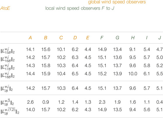
TABLE 3. Mean Euclidean norm $\Vert L_{i\mathcal{B}}^{w,\bar{j}}{\Vert }_2$ and average, mean Euclidean norm $\Vert L_{\bar{i}\mathcal{B}}^{w,\bar{j}}{\Vert }_2$ of the error-feedback gain matrices L_i(v_i) of the $\text{global wind speed} \text{observers}$ $A \text{to} E$ (i.e., w ∈ [A, E]) and $\text{local wind speed observers}F\text{to}J$ (i.e., w ∈ [F, J], see Table A8) for increasing upper bounds ${\alpha }_{\mathcal{B},\max }$ (with $\Vert L_{\bar{i}\mathcal{B}}^{w,\bar{3}}{\Vert }_2$ for the average, mean Euclidean norm of the wind model error-feedback gains (j = 3) and $\Vert L_{\bar{i}\mathcal{B}}^{w,\overline{(\mathrm{1,2})}}{\Vert }_2$ for the average, mean Euclidean norm of the $\mathcal{B}$lade error-feedback gains (j = 1,2))

Membership functions

To visualise the convex blending of direct adjacent submodels (A_i, B_i), the time series of the membership functions h_i for a step-shaped wind time series are depicted in Figure 5. Note: As the premise variable in this contribution is defined by one parameter $(\underline{z}\equiv \widehat{v})$, the membership function h_i(z) is identical to the weighting function w_k,l(z) (see Section 2.4.3, especially footnote⁴). Therefore, just two submodels are blended at the same time (for all operating points between two steady state operating points OP_i; see also the triangular-shaped h_i(z) progression (with h_i(z) ≡ w_k,l (z_k) for z_k = z₁ = z with k_max = 1) in Figure 1).

FIGURE 5

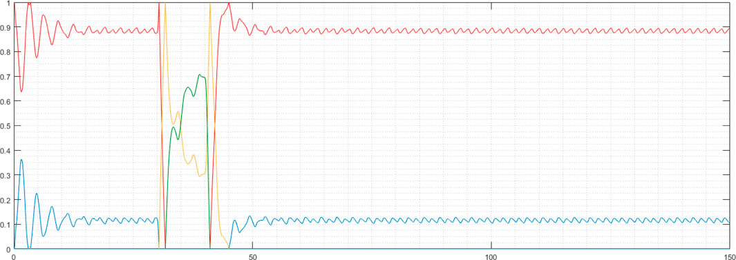
FIGURE 5. Exemplarily time series of the membership functions h_i for the $\text{global wind speed observer}A$ (with i ∈[15,18]) for the step-shaped wind time series depicted in Figure 6.

Wind turbine simulations, actuation signals, pitch rate deviations, rotation speed deviations and resulting mechanical loads

To assess the closed-loop system dynamics (see Figure 6), a disturbing step-shaped time series of 150 s duration is applied to the system, visualising the effect of the particular wind speed observer design (with decreased performance, see Section 3.1) on the actuation signals. The resulting time series ${\widehat{v}}^w(t)$, ${\beta }_{FF}^w(t)$ and ${\beta }_{FB}^w(t)$ were achieved with NREL FAST 5 MW reference wind turbine simulations, embedded in a Matlab Simulink model, using the wind speed observer-based PDC controller Eq. 5 (i.e., for all simulations the same PDC feedback-controller⁸ is utilised) with step-shaped wind time series as disturbing excitation. For clarity, the simulations are restricted to the full load range with pitch angle actuation, i.e., the generator torque is kept constant (see Section 2.4.2 and Table A1).

FIGURE 6

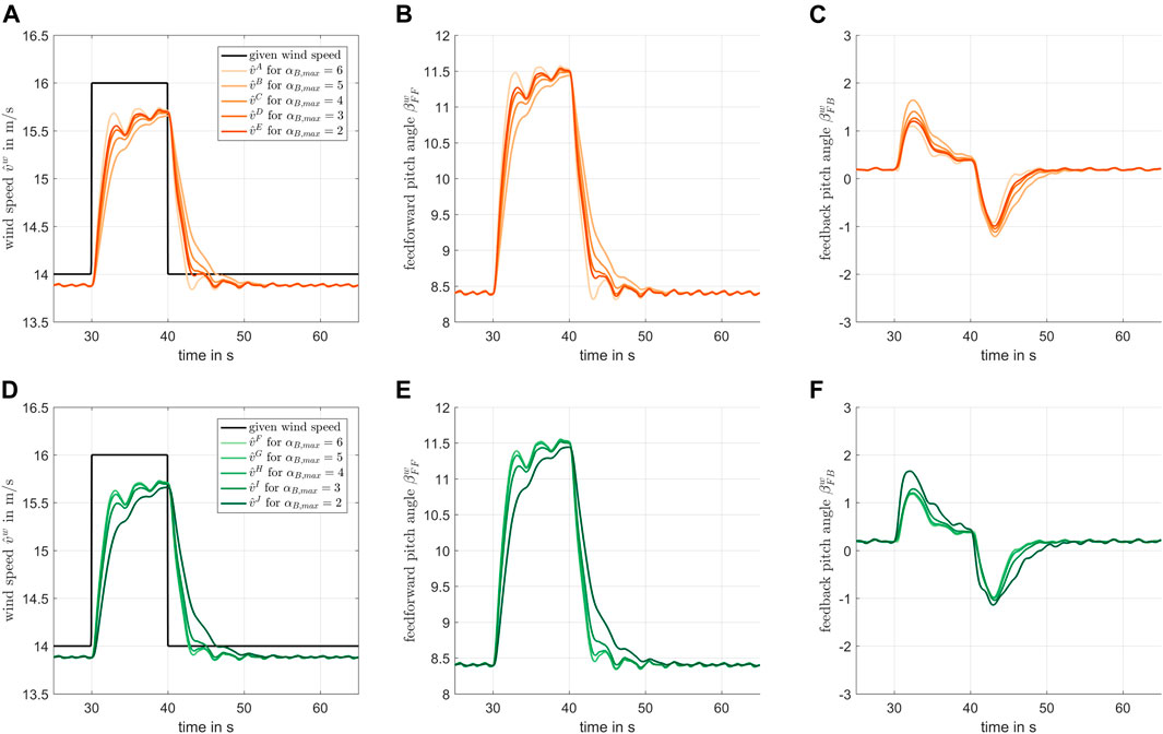
FIGURE 6. Time series segment of wind speed reconstruction $\widehat{v}$ (left column), feedforward pitch actuation β_FF (mid column) and feedback pitch actuation β_FB (right column), with the observer-based controller and step disturbance signals for an increasing upper bound ${\alpha }_{\mathcal{B},\max }$ resulting in shrinking pole regions, applied to the $\text{global Lyapunov approach}$ (with w ∈ [A, E], see upper subplots) and $\text{local Lyapunov approach}$ (with w ∈ [F, J], see lower subplots).

The given wind speeds v and the reconstructed wind speeds ${\widehat{v}}^w$ of the step-shaped wind time series are depicted in the left column of Figure 6, the actuated feedforward and feedback pitch angles ${\beta }_{FF}^w(t)$ and ${\beta }_{FB}^w(t)$ are depicted in the mid and right column of Figure 6. The resulting ultimate and mean pitch angle deviations, i.e. the pitch rates $\text{max}(\dot{\beta })$ and $\text{mean}(\dot{\beta })$ are depicted in the left column of Figures 7A,B; the closed-loop system dynamics, i.e. the ultimate and standard drive train rotation speed deviations $\text{max}(\mathrm{\Delta }\omega )=\text{max}(\frac{\omega -{\omega }_r}{{\omega }_r})$ and $\text{std}(\mathrm{\Delta }\omega )=\text{std}(\frac{\omega -{\omega }_r}{{\omega }_r})$ (with the rated rotation speed ω_r), are depicted in the right column of Figures 7A,B.

FIGURE 7

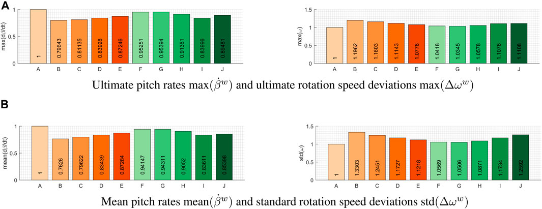
FIGURE 7. Actuation speed and pitch angle deviations, respectively (so called pitch rate $\dot{\beta }=d\beta /dt$), i.e. ultimate $\text{max}({\dot{\beta }}^w)$ and mean $\text{mean}({\dot{\beta }}^w)$ pitch rates for the $w\in \left[A,E\right]\hspace{0.17em}\text{global wind speed observers and}$ $w\in \left[F,J\right]\hspace{0.17em}\text{local wind speed observers}$ (normalised to $\text{max}({\dot{\beta }}^A)$ and $\text{mean}({\dot{\beta }}^A)$; see left column of subplot A,B). Rotation speed deviations Δω^w (with $\mathrm{\Delta }{\omega }^w=\frac{{\omega }^w-{\omega }_r}{{\omega }_r}$ and the rated rotation speed ω_r), i.e. ultimate max(Δω^w) and standard std(Δω^w) rotation speed deviations [normalised to max(Δω^A) and std(Δω^A); see right column of subplot A,B]. The ultimate deviations $\text{max}({\dot{\beta }}^w)$ and max(Δω^w) (see subplot A) result from the ultimate load analysis and the mean deviations $\text{mean}({\dot{\beta }}^w)$ and standard deviations std(Δω^w) (see subplot B) result from the fatigue load analyses of the step-shaped wind time series, depicted in Figure 8.

In addition, the step-shaped wind time series – representing a typical wind increase and wind decrease event (i.e. a disturbing step up and step down signal) within a turbulent wind excitation time series – is used to assess the ultimate and fatigue loads resulting from the closed-loop system dynamics of both approaches. For this load assessment, five different loads are analysed that are crucial or at least very important for the wind turbine’s main component design of tower, blades and the drive train:

• The tower bending moment in wind direction (also denoted with the fore-aft bending moment, TwrBsMyt) and normal to the wind direction (also denoted with the side-to-side bending moment, TwrBsMxt), calculated for the tower base,

• the blade bending moment in wind direction (i.e., resulting from blade bending out of the rotor plane, also denoted with the flapwise or out-of-plane bending moment, RootMyb1) and blade bending moment inside the rotor plane (edgewise or in-plane bending moment, RootMxb1), calculated for the blade root (next to the hub body) of the first blade, and

• the torsional torque (ΔTq) along the drive train axis.

The ultimate and fatigue loads, resulting from the closed-loop system dynamics, are depicted in Figure 8. To eliminate effects, resulting from simulation initialisation, the time period 0s ≤ t_CutOff ≤ 10s of all time series is not taken into account in the load evaluation. (Note: If the fatigue loads in Figure 8 just differ even in the third or fourth decimal place, these differences are of significance. Because, the listed fatigue loads in Figure 8 result from a wind times series of extremely short duration (of 150 s), while wind turbines typically operate for 20 years with approximately 97% availability. That is, also fourth decimal place differences in the fatigue loads, depicted in Figure 8, do have an enormous impact on the expected wind turbine lifetime, as all damages cumulate over the complete lifetime. This cumulation does not apply to ultimate loads, as these loads occur rarely in a wind turbine’s lifetime).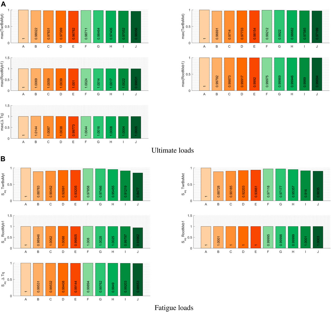

FIGURE 8

FIGURE 8. Ultimate loads max^w (…) and fatigue loads $S_{eq}^w(\dots )$ (also denoted with Damage Equivalent Loads or Damage Equivalent Amplitudes S_eq) resulting from the closed-loop dynamics of a step-shaped wind time series with a mean wind speed of $\bar{v}=14m/s$ (see Figure 6), for the $w\text{different global wind speed observers}$ $(\text{resulting from the global Lyapunov design approach with}w\in \left[A,,,E\right])$ and the $w\hspace{0.17em}\text{local wind speed observers}\text{(resulting from the local Lyapunov design approach with}\hspace{0.17em}w$$\in \left[F,J\right])$, normalised to the ultimate load max^A (…) or fatigue load $S_{eq}^A(\dots )$ of the global wind speed observer A. For the ultimate and fatigue loads, the tower bending moment TwrBsMyt and TwrBsMxt (at the tower base—top row), the blade bending moment RootMyb1 and RootMxb1 (at the blade root section—mid row) and the drive train torque ΔTq (bottom row) are depicted.

4 Discussion

Both Lyapunov approaches fulfill the particular objective to decrease the disturbance observer performance and feedforward actuation, while increasing the feedback actuation for shrinking pole region dimensions, resulting in mitigated mechanical loads (see Section 3.1). But the local approach achieves significantly increased flexiblity and consistency of the desired and resulting system dynamics than the global approach:

Pole locations

The open-loop poles of the wind turbine system, depicted with gray symbols in Figure 4, are widely spaced, as significant distances between the real-valued wind model poles $s_{P,i}^{OL,1}$ (on the real axis of the pole map) and the conjugated-complex blade poles $s_{P,i}^{OL,2\vee 3}$ (in the pole map) exist. With increasing upper bounds ${\alpha }_{\mathcal{B},\max }$, resulting in shrinking pole regions⁹, the closed-loop pole locations $s_{P,i}^{w,p}$ are shifted for both design approaches inside the left half of the pole map in direction of the imaginary axis and towards the open-loop poles $s_{P,i}^{OL,p}$. Thereby, the average distances $\mathrm{\Delta }{s}_{P,\bar{i}}^{w,\bar{p}}$ in the complex pole map decrease (i.e., $\mathrm{\Delta }{s}_{P,\bar{i}}^{w,\bar{p}}>\mathrm{\Delta }{s}_{P,\bar{i}}^{(w+1),\bar{p}}$, e.g., $\mathrm{\Delta }{s}_{P,\bar{i}}^{B,\bar{p}}>\mathrm{\Delta }{s}_{P,\bar{i}}^{C,\bar{p}}$, see Figure 4 and Table 2). Just for the last global and local wind speed observers the distances increase, i.e., $\mathrm{\Delta }{s}_{P,\bar{i}}^{D,\bar{p}}<\mathrm{\Delta }{s}_{P,\bar{i}}^{E,\bar{p}}$ and $\mathrm{\Delta }{s}_{P,\bar{i}}^{I,\bar{p}}<\mathrm{\Delta }{s}_{P,\bar{i}}^{J,\bar{p}}$, as the closed-loop poles (and their real-values $\mathrm{R}\mathrm{e}(s_{P,i}^{w,p})$, respectively) are shifted beyond the open-loop poles $\mathrm{R}\mathrm{e}(s_{P,i}^{OL,p})$ in direction of the imaginary axis. Therefore, those two wind speed observers E and J are not accounted in the following evaluations, but they are relevant for the local approach assessment, as described in the following with regard to the pole region violation.—For the wind speed observer poles, based on the local Lyapunov approach (see w ∈ [F, I] in Table 2), the pole distances $\mathrm{\Delta }{s}_{P,\bar{i}}^{w,\bar{p}}$ decrease steadily, while the distances $\mathrm{\Delta }{s}_{P,\bar{i}}^{w,\bar{p}}$ for the wind speed observer poles, based on the global Lyapunov approach (see w ∈ [A, D]), show a local maximum for the wind speed observer B (i.e., $\mathrm{\Delta }{s}_{P,\bar{i}}^{B,\bar{p}}>\mathrm{\Delta }{s}_{P,\bar{i}}^{A,\bar{p}}>\mathrm{\Delta }{s}_{P,\bar{i}}^{C,\bar{p}}>\mathrm{\Delta }{s}_{P,\bar{i}}^{D,\bar{p}}$). Thus, the local Lyapunov approach is rated to be more coincident in regard to a desired pole location specification. Additionally, it is obvious from the pole locations depicted in Figure 4, that the local Lyapunov approach is more effective and flexible, respectively, as all poles are located inside the specified pole regions, while the global Lyapunov approach is not able to satisfy the pole region specifications for the smallest pole region, resulting in poles located outside the specified pole regions (see the pole location $s_{P,i}^{E,p}$ of the global wind speed observer E in Figure 4E). That is, the local Lyapunov approach is more flexible in assigning desired pole locations than the global Lyapunov approach.

(Note, that the LMI solver is capable to find solutions, even if the pole region LMIs are violated. However, the resulting poles are still located in the left half of the complex pole map and fulfill the basic stability condition for the corresponding closed-loop or error dynamics.)

Error-feedback gains

With the decreasing pole distances $\mathrm{\Delta }{s}_{P,\bar{i}}^{w,\bar{p}}$, also the error-feedback gains $L_{i\mathcal{B}}^{w,j}$—representing a measure or the effort of all error states acting on the wth observer—are mitigated. For all¹⁰ local wind speed observer designs these gains decrease expectedly with increasing upper bound ${\alpha }_{\mathcal{B},\max }$ and with the reduced pole distances $\mathrm{\Delta }{s}_{P,\bar{i}}^{w,\bar{p}}$ (i.e., $\Vert L_{\bar{i}\mathcal{B}}^{F,\bar{j}}{\Vert }_2>\Vert L_{\bar{i}\mathcal{B}}^{G,\bar{j}}{\Vert }_2>\Vert L_{\bar{i}\mathcal{B}}^{H,\bar{j}}{\Vert }_2>\Vert L_{\bar{i}\mathcal{B}}^{I,\bar{j}}{\Vert }_2$). Corresponding to the pole distances $\mathrm{\Delta }{s}_{P,\bar{i}}^{w,\bar{p}}$, the local wind speed observer gains $L_{i\mathcal{B}}^{w,j}$ are mitigated steadily (and yield lower gains $\Vert L_{\bar{i}\mathcal{B}}^{B,\bar{j}}{\Vert }_2>\Vert L_{\bar{i}\mathcal{B}}^{G,\bar{j}}{\Vert }_2,\Vert L_{\bar{i}\mathcal{B}}^{C,\bar{j}}{\Vert }_2>\Vert L_{\bar{i}\mathcal{B}}^{H,\bar{j}}{\Vert }_2\text{and}\Vert L_{\bar{i}\mathcal{B}}^{D,\bar{j}}{\Vert }_2>\Vert L_{\bar{i}\mathcal{B}}^{I,\bar{j}}{\Vert }_2$), while the global wind speed observer gains show a local maximum of $\Vert L_{\bar{i}\mathcal{B}}^{w,\bar{j}}{\Vert }_2$ for the wind speed observer B (i.e., $\Vert L_{\bar{i}\mathcal{B}}^{B,\bar{j}}{\Vert }_2>\Vert L_{\bar{i}\mathcal{B}}^{A,\bar{j}}{\Vert }_2>\Vert L_{\bar{i}\mathcal{B}}^{C,\bar{j}}{\Vert }_2>\Vert L_{\bar{i}\mathcal{B}}^{D,\bar{j}}{\Vert }_2$), demonstrating the increased consistency of the desired and achieved error-feedback gains $L_{i\mathcal{B}}^{w,j}$ of the local Lyapunov approach.

Wind speed reconstruction and actuation signals

With the mitigated error-feedback gains $L_{i\mathcal{B}}^{w,j}$, the reconstructed states $\underline{\widehat{x}}$, especially the reconstructed wind speeds $\widehat{v}$, are mitigated, too (see Eq. 7¹¹): While the reconstructed wind speed ${\widehat{v}}^w(t_1)$ of a single and arbitrary time point t = t₁ decreases steadily for the wind speed observer design with local Lyapunov approach (i.e., ${\widehat{v}}^F(t_1)\approx {\widehat{v}}^G(t_1)>{\widehat{v}}^H(t_1)>{\widehat{v}}^I(t_1)[>{\widehat{v}}^J(t_1)]$¹⁰, see left column in Figure 6), the reconstructed wind speed ${\widehat{v}}^w(t_1)$ for the wind speed observer design with global Lyapunov approach decreases unsteadily (i.e., ${\widehat{v}}^A(t_1)>{\widehat{v}}^D(t_1)[>{\widehat{v}}^E(t_1)]>{\widehat{v}}^C(t_1)>{\widehat{v}}^B(t_1)$, corresponding to the unsteady decrease of the mean Euclidean norm of the wind error state gains $\Vert L_{\bar{i}\mathcal{B}}^{w,\bar{\mathit{3}}}{\Vert }_2$ of the global wind speed observers (with w [A, E], see Table 3; i.e., $\Vert L_{\bar{i}\mathcal{B}}^{A,\bar{3}}{\Vert }_2>\Vert L_{\bar{i}\mathcal{B}}^{D,\bar{3}}{\Vert }_2>\Vert L_{\bar{i}\mathcal{B}}^{C,\bar{3}}{\Vert }_2>\Vert L_{\bar{i}\mathcal{B}}^{B,\bar{3}}{\Vert }_2$)¹⁰.

The mitigated, reconstructed wind speeds ${\widehat{v}}^w$ of both approaches result in the following actuation signals: The mitigated wind speeds ${\widehat{v}}^w$ lead to less dominant feedforward pitch actuation β_FF—just governed by the wind speed driven feedforward actuation ${\underline{u}}_{FF}(h_j(\underline{z}))$ (with u_FF ≡ β_FF and $\underline{z}\equiv {\widehat{v}}^w$) according to Eq. 5 and the steady state pitch angles β_c,i (listed in Table A1)—and increase the feedback pitch angles β_FB (see mid and right column in Figure 6). That is, corresponding to the decreased, reconstructed wind speeds ${\widehat{v}}^w$ (and mean wind state feedback gains $\Vert L_{\bar{i}\mathcal{B}}^{w,\bar{\mathbf{3}}}{\Vert }_2$), the feedforward pitch angles of the local wind speed observers ${\beta }_{FF}^w$ (with w ∈ [F, I]¹⁰) are mitigated steadily (i.e., ${\beta }_{FF}^F\approx {\beta }_{FF}^G>{\beta }_{FF}^H>{\beta }_{FF}^I[>{\beta }_{FF}^J]$, see mid column in Figure 6) and yield steadily increased feedback pitch angles (i.e., ${\beta }_{FB}^F<\dots <{\beta }_{FF}^I[<{\beta }_{FB}^J]$, see right column in Figure 6), while the feedforward pitch angles of the global wind speed observers ${\beta }_{FF}^w$ (with w ∈ [A, D]) decrease unsteadily (i.e., ${\beta }_{FF}^A<{\beta }_{FF}^D<{\beta }_{FF}^C<{\beta }_{FF}^B$) and yield correspondingly increasing feedback pitch angles ${\beta }_{FB}^w$ (with w ∈ [A, D]). Thus, the intended particular objective of a steadily decreasing feedforward-actuation with increasing feedback-compensation (see Section 3.1) is achieved with the local, not with the global Lyapunov wind speed observer design approach.

Pitch rate deviations and rotation speed deviations

The pitch angle deviations result in corresponding pitch and rotation speed metrics: With the steadily mitigated premise variable ${\widehat{v}}^F>{\widehat{v}}^G>{\widehat{v}}^H>{\widehat{v}}^I$ of the local wind speed observer F to I, the ultimate pitch rates $\text{max}(\dot{\beta })(=\text{max}({\dot{\beta }}_{FF}+{\dot{\beta }}_{FB})\mathrm{w}\mathrm{i}\mathrm{t}\mathrm{h}\text{max}({\dot{\beta }}^F)\approx \text{max}({\dot{\beta }}^G)>\text{max}({\dot{\beta }}^H)>\text{max}({\dot{\beta }}^I))$ and mean pitch rates $\text{mean}(\dot{\beta })$ (with $\text{mean}({\dot{\beta }}^F)\approx \text{mean}({\dot{\beta }}^G)>\text{mean}({\dot{\beta }}^H)>\text{mean}({\dot{\beta }}^I)$) decrease steadily, too (see left column in Figures 7A,B), while the unsteadily decreasing wind speeds ${\widehat{v}}^A>{\widehat{v}}^D>{\widehat{v}}^C>{\widehat{v}}^B$ of the global wind speed observers A to D lead to unsteadily decreasing ultimate pitch rates $\text{max}({\dot{\beta }}^A)>\text{max}({\dot{\beta }}^D)>\text{max}({\dot{\beta }}^C)>\text{max}({\dot{\beta }}^B)$ and mean pitch rates $\text{mean}({\dot{\beta }}^A)>\text{mean}({\dot{\beta }}^D)>\text{mean}({\dot{\beta }}^C)>\text{mean}({\dot{\beta }}^B)$. As the pitch rates $\dot{\beta }$ decrease, increasing system dynamic deviations appear, e.g. represented by the metric of the drive train rotation speed deviations max(Δω) and std(Δω), that increase steadily for the local wind speed observers (with max(Δω^F) ≈ max(Δω^G) and std(Δω^F) ≈ std(Δω^G)) and unsteadily for the global wind speed observers (see right column in Figure 7 A,B). Thus, the local Lyapunov approach achieves the expected system dynamics with increased consistency between the desired and achieved pitch rate deviations and rotation speed deviations, compared to the global Lyapunov approach.

Load mitigation

The ultimate and fatigue loads resulting from closed-loop dynamics with the step-shaped wind excitation (depicted in Figure 8) are satisfying for both approaches, but especially for the local Lyapunov approach. In the following, the ultimate and fatigue loads are first evaluated separately for each of the two Lyapunov approaches (see Table A9), then the loads from both approaches are compared with each other (see Table A10).

• Ultimate Loads (see Figure 8A): The ultimate tower bending moments max(TwrBsMyt) and max(TwrBsMxt), as well as the ultimate in-plane blade bending moments max(RootMxb1) are mitigated for both Lyapunov approaches, and for the local Lyapunov approach these ultimate loads decrease even steadily (see lines 1 to 3 in Table A9; with one marginal exception for max^F(TwrBsMxt) < max^G(TwrBsMxt)). The ultimate out-of-plane blade bending moments max(RootMyb1) and the ultimate drive train torque max(ΔTq) increase slightly, but not significantly (see Figure 8A and lines 4 to 5 in Table A9). – Comparing both approaches with each other, for most pole regions lower ultimate loads are achieved with the local Lyapunov design approach (see Figure 8B and lines 1 to 5 in Table A10).

  If a controller variation yields comparable or even lower ultimate loads, the controller (design approach) assessment depends on the fatigue loads.

• Fatigue Loads (see Figure 8B): The fatigue tower bending moments S_eq(TwrBsMyt) and S_eq(TwrBsMxt), as well as the fatigue drive train torque S_eq(ΔT) are mitigated for both Lyapunov approaches, and for the local Lyapunov approach these fatigue loads decrease steadily (see lines 6 to 8 in Table A9; with one exception for $S_{eq}^F(TwrBsMxt)<S_{eq}^G(TwrBsMxt)$). The fatigue out-of-plane blade bending moments S_eq(RootMyb1) and in-plane blade bending moments S_eq(RootMxb1) increase slightly, but for the local Lyapunov approach the out-of-plane blade bending fatigue loads $S_{eq}^w(RootMyb1)$ decrease steadily (see Figure 8B and lines 9 to 10 in Table A9). – Comparing both approaches with each other, for most pole regions lower fatigue loads are achieved with the local Lyapunov design approach, again (see Figure 8B and lines 6 to 10 in Table A10).

  Additionally, the local wind speed observer design approach with the smallest pole region (see wind speed observer J) achieves the lowest fatigue loads for those bending moments and torsional torque compared to the fatigue loads, resulting from the global wind speed observer design (compare the fatigue loads of local wind speed observer J with the fatigue loads of all global wind speed observers for S_eq(TwrBsMyt), S_eq(TwrBsMxt)¹², S_eq(RootMyb1) and S_eq(ΔTq) in Figure 8). – Just the in-plane blade fatigue bending moments S_eq(RootMxb1) increase for the local wind speed observer design approach (as well as for the global approach). This fatigue load increase might result from the increasing rotation speed deviations max(Δω) and std(Δω). Because, for identical wind times series and system excitations, respectively, increasing fatigue loads result from increasing amplitude and/ or increasing load cycles. As the rotation speed deviations max(Δω) and std(Δω) increase with the shrinking pole region dimension (see max(Δω) and std(Δω) for WindObs w with w ∈ [G, J] in the right column of Figures 7A,B), it seems reasonable, that the fatigue load increase results from the increasing rotation speed, rather than from an amplitude increase. This assumption is also confirmed by the ultimate loads that decrease with the shrinking pole region size (see max(RootMxb1) for WindObs w with w ∈ [F, J] in Figure 8), i.e. not the amplitudes of ultimate and fatigue loads, but the load cycles of the fatigue loads increase. Additionally, with the increasing rotor speed deviations, the number of blade passages through the tower shadow¹³ increases, resulting in increasing load cycles and leading to increased fatigue loads.

Therefore, it seems promising as a subject of future work, to split the wind speed observer, based on a local Lyapunov approach, into two, separated wind speed observers: A feedforward wind speed observer—specified with a similar pole region (like wind speed observer I, used within this contribution)—with decreased reconstruction performance to assign the premise variable ${\widehat{v}}_{FF}$ to the feedforward actuation ${\underline{u}}_{FF}(h({\widehat{v}}_{FF}))$. To compensate the decreased feedforward pitch rates ${\dot{\beta }}_{FF}$, an additional feedback wind speed observer with increased performance will be implemented, to assign its reconstructed wind speed ${\widehat{v}}_{FB}$ to the feedback actuation. For this feedback wind speed observer, a tight pole region will be specified, located left from the open-loop poles, resulting in significantly increased error-feedback gains L_i,FB and reconstructed wind speeds ${\widehat{v}}_{FB}$, so that the feedback pitch rates ${\dot{\beta }}_{FB}$ increase, resulting in mitigated rotation speed deviations and fatigue loads. Summing up the load evaluation, the local Lyapunov approach is rated to gain an increased consistency between intended and achieved load mitigation compared to the global approach. While the ultimate loads, achieved with the global and local wind speed observer approach are comparable, the local approach achieves an increased fatigue load mitigation. Because, for steadily shrinking pole regions with steadily decreasing feedforward actuation, the fatigue loads decrease steadily, too.

5 Conclusion

With this contribution a local Lyapunov approach is introduced for controller and observer design in the Takagi-Sugeno framework. Compared to the common global Lyapunov approach, a more dedicated closed-loop dynamic is intended with the local Lyapunov approach, i.e., an increased flexibility in the design process and increased consistency between desired and achieved system dynamics is aspired.

The applicability and effectiveness of the local Lyapunov approach to wind turbine control is analysed with wind turbine simulations. The simulation results show, that the local Lyapunov approach makes it possible to influence the pole locations, the resulting error-feedback gains and closed-loop system dynamics more flexible and with an increased consistency between desired and achieved system dynamics than the global Lypunov approach. That is, with the local Lyapunov approach, the assignment of smaller pole regions is possible, enabling a higher flexibility in assigning desired system dynamics. Additionally, the local Lyapunov approach reaches an improved similarity between the desired and achieved closed-loop system dynamics, indicating the increased consistency of the local Lyapunov approach. As the local Lyapunov approach is less conservative, but more dedicated to the desired system dynamics, i.e., the design process achieves an increased flexibility and increased consistency, it is rated to have a higher potential in fulfilling primary and secondary control objectives, like energy yield optimisation and load mitigation in wind turbine application.

The evaluation of the local Lyapunov approach will be continued in oncoming studies, with the controller structure adapted to the new possibilities arising from the local design approach, like the separated reconstruction of the feedforward and the feedback premise variable in a split wind speed observer.

Data Availability Statement

The original contributions presented in the study are included in the article/Supplementary Material, further inquiries can be directed to the corresponding author.

Author Contributions

Eckhard Gauterin and Horst Schulte devised the basic Takagi-Sugeno observer-based feedforward control concept for wind turbine control and conceptualized this study. Florian Pöschke developed the linearised wind turbine model in Takagi-Sugeno framework and conceived the local Lyapunov approach. Florian Pöschke expedited the implementation and development of the control concept in the simulation software, while Eckhard Gauterin conducted the simulation studies. All three authors analysed the results and Eckhard Gauterin created the manuscript, that was reviewed by all three authors.

Conflict of Interest

The authors declare that the research was conducted in the absence of any commercial or financial relationships that could be construed as a potential conflict of interest.

Publisher’s Note

All claims expressed in this article are solely those of the authors and do not necessarily represent those of their affiliated organizations, or those of the publisher, the editors and the reviewers. Any product that may be evaluated in this article, or claim that may be made by its manufacturer, is not guaranteed or endorsed by the publisher.

Footnotes

¹With individual input matrices B_i a weighted combination of the ith submodel with all and the direct adjacent submodels (see Section 2.1.1), respectively, is derived for the closed-loop dynamics, due to the individual weighting ${\sum }_i{h}_i(\underline{z})B_i$ of the individual input matrices B_i for each submodel. Therefore, the double summation ∑_i ∑_j is necessary in Eq. 6.

²With a common output matrix C_i ≡ C the weighted combination of the ith submodel with all and the direct adjacent submodels, respectively, is superfluous for the reconstructed closed-loop dynamics, as ${\sum }_i{h}_i(\underline{z})C=C{\sum }_i{h}_i(\underline{z})=C\cdot 1=C$ holds for all submodel. Therefore, the single summation ∑_i is sufficient in Eq. 7 and Eq. 9.

³Note: Within this contribution just the blade tip translations $x_{\mathcal{B},1/2/3}$ are assumed to be measurable, whereat the mean value $x_{\mathcal{B}}=(1/3)(x_{\mathcal{B},1}+x_{\mathcal{B},2}+x_{\mathcal{B},3})$ is utilised for calculating the error $e_{\mathcal{B}}=x_{\mathcal{B}}-{\widehat{x}}_{\mathcal{B}}$, fed back and amplified with the error gains L_i to reconstruct the blade tip speed ${\dot{\widehat{x}}}_{\mathcal{B}}$, blade tip acceleration ${\ddot{\widehat{x}}}_{\mathcal{B}}$ and temporal wind speed variations ${\dot{\widehat{v}}}_{\mathcal{B}}$.

⁴The triangular shape of the membership functions holds, if just one premise variable z_k = z (with k = k_max = 1) is defined. Because in this case, the membership function h_i(z) (Eq. 1) is identical to the triangular-shaped weighting function w_k,l(z), see Eq. 2.

⁵These brisk feedforward-actuation result from feedforward specifications without dynamics (i.e., without any damping influence, e.g., from the K_i gains), but simple convex blending of the steady states ${\underline{u}}_{c,j}$ (see ${\underline{u}}_{FF}$ in Eq. 5).

⁶with ${\sum }_i^{Nr}{h}_i(\widehat{v})L_{i}C\left(\underline{x}-\widehat{\underline{x}}\right)=\underset{=:L(\widehat{v})}{\underbrace{{\sum }_i^{Nr}{h}_i(\widehat{v})L_i}}C\underline{e}=L(\widehat{v})C\underline{e}$, see Eq. 7 (with $\underline{z}\equiv \widehat{v}$) and Eq. 8.

⁷As the pole location distance $\mathrm{\Delta }{\text{s}}_{\text{P},\text{i}}^{\text{w},\text{p}}$ depends on the difference between $s_{P,i}^{OL,p}$ and $s_{P,i}^{w,p}$ (i.e., $\mathrm{\Delta }{s}_{P,i}^{w,p}=f(s_{P,i}^{OL,p}-s_{P,i}^{w,p})$, see Section 3.2 with $s_{P,i}^{OL,p}=eig(A_i)$ and $s_{P,i}^{w,p}=eig(A_i-L_i^{w}C)$, i.e., $\mathrm{\Delta }{s}_{P,i}^{w,p}=f(eig(A_i)-eig(A_i-L_i^{w}C))$), this distance $\mathrm{\Delta }{s}_{P,i}^{w,p}$ in-/decreases, if the error-feedback gain $L_i^w$ in-/decreases—and vice versa, i.e., $L_i^w$ in-/decreases for in-/decreasing $\mathrm{\Delta }{s}_{P,i}^{w,p}$.

⁸PDC feedback controller: ct1010001

⁹to realise the shrinking pole region size, compare the pole regions’ size (and location) in Figure 4 for the wind speed observer design A and F with E and J

¹⁰The global and local wind speed observers E and J are not taken into account, because of their (closed-loop) pole locations, which are moved beyond the open-loop pole locations, as explained before in the subsection Pole locations.

¹¹If Eq. 7 is evaluated for a single and arbitrary time point, it is obvious, that $\underline{\dot{\widehat{x}}}$ (and $\underline{\widehat{x}}$) decreases, if $L_{i\mathcal{B}}^{w,j}$ is mitigated, while all other parameters and states do not change.

¹²with two exceptions for the tower side-to-side-bending moments $S_{eq}^B(TwrBsMxt)<S_{eq}^J(TwrBsMxt)$ and $S_{eq}^C(TwrBsMxt)<S_{eq}^J(TwrBsMxt)$ (see Figure 8B and line 7 in Table A9 as well as line 7 in Table A10.

¹³Tower shadow (effect): The tower poses as an obstacle in the inflow that increases the dynamic pressure and decreases the wind speed in front, i.e. in upwind direction of the tower.

¹⁴with two exceptions for the tower side-to-side-bending moments $S_{eq}^B(TwrBsMxt)<S_{eq}^C(TwrBsMxt)<S_{eq}^J(TwrBsMxt)$

¹⁵Tower shadow (effect): The tower poses as an obstacle in the inflow that increases the dynamic pressure and decreases the wind speed in front, i.e., in upwind direction of the tower

References

Bianchi, F. D., De Battista, H., and Mantz, R. J. (2007). Wind turbine control systems - principles, modelling and gain scheduling design. London, United Kingdom: Springer-Verlag, London Limited.

Google Scholar

Bossanyi, E. A. (2000). The design of closed loop controllers for wind turbines. Wind Energy (Chichester). 3, 149–163. doi:10.1002/we.34

CrossRef Full Text | Google Scholar

Boyd, S., El Ghaoui, L., Feron, E., and Balakrishnan, V. (1994). Linear matrix inequalities in system and control theory. Philadelphia: SIAM.

Google Scholar

Chilali, M., and Pascal, G. (1996). H_∞ design with Pole placement constraints: an LMI approach. IEEE Trans. Autom. Contr. 41, 358–367. doi:10.1109/9.486637

CrossRef Full Text | Google Scholar

Clemens, C., Gauterin, E., Pöschke, F., and Schulte, H. (2020). “Assessment criteria for the mechanical loads of wind turbines applied to the example of active power control, s. 1-7, berlin, Germany,” in Proceedings of IFAC World Congress 2020, Berlin, Germany, 341–347.

CrossRef Full Text | Google Scholar

Ekelund, T. (1994). “Speed control of wind turbines in the stall region,” in IEEE conference on control applications (Glasgow, United Kingdom), 227–232.

CrossRef Full Text | Google Scholar

Gauterin, E., Kammerer, P., Martin, K., and Schulte, H. (2015). Effective wind speed estimation: comparison between kalman filter and takagi-sugeno observer techniques. ISA-Transactions 62, 60–72.

PubMed Abstract | CrossRef Full Text | Google Scholar

Gauterin, E., Schulte, H., and Georg, S. (2014). Disturbance compensation by wind speed reconstruction based on a takagi-sugeno wind turbine model. J. Phys. Conf. Ser. 524, 012072. Proceedings ‘The Science of Making Torque from Wind 2014’. IOP Publishing. doi:10.1088/1742-6596/524/1/012072

CrossRef Full Text | Google Scholar

Georg, S. (2015). Fault diagnosis and fault-tolerant control of wind turbines nonlinear Takagi-Sugeno and sliding mode techniques. PhD thesis. Rostock, Germany: University Rostock, Fakultät für Maschinenbau und Schiffstechnik.

Google Scholar

Jena, D., and Rajendran, S. (2015). A review of estimation of effective wind speed based control of wind turbines. Renew. Sustain. Energy Rev. 43, 1046–1062. doi:10.1016/j.rser.2014.11.088

CrossRef Full Text | Google Scholar

Johansen, T. A., Shorten, R., and Murray-Smith, R. (2000). On the interpretation and identification of dynamic takagi-sugeno fuzzy models. IEEE Trans. Fuzzy Syst. 8 (3), 297–313. doi:10.1109/91.855918

CrossRef Full Text | Google Scholar

Jonkman, J. (2016). NWTC Design Codes (FAST). v8.16 edition. Golden, CO: National Renewable Energy Laboratory (NREL).

Google Scholar

Jonkman, J. B., and Jonkman, B. J. (2016). “Fast modularization framework for wind turbine simulation: full-system linearization,” in The science of making torque from wind, Vol. 753, 082010.

CrossRef Full Text | Google Scholar

Jonkman, J., Butterfield, S., Musial, W., and Scott, G. (2009). Definition of a 5-MW reference wind turbine for offshore system development. Technical report, NREL/TP-500-38060. Golden, Colorado: National Renewable Energy Laboratory.

Google Scholar

Jonkman, J. M., and Buhl, M. L. (2005). FAST user’s guide. Technical report, NREL/EL-500-38230. Golden, Colorado: National Renewable Energy Laboratory.

Google Scholar

Lendek, Z., Guerra, T. M., Babuška, R., and De Schutter, B. (2010). Stability analysis and nonlinear observer design using takagi-sugeno fuzzy models. Berlin: Springer-Verlag Berlin Heidelberg.

Google Scholar

Li, S., Yang, J., Chen, W.-H., and Chen, X. (2014). Disturbance observer-based control: Methods and applications. 1st edition. Boca Raton: CRC Press Taylor and Francis Group.

Google Scholar

Luenberger, D. G. (1971). An introduction to observers. IEEE Trans. Autom. Contr. 16, 596–602. doi:10.1109/tac.1971.1099826

CrossRef Full Text | Google Scholar

Luenberger, D. G. (1964). Observing the state of a linear system. IEEE Trans. Mil. Electron. 8, 74–80. doi:10.1109/tme.1964.4323124

CrossRef Full Text | Google Scholar

Lyapunov, A. M. (1992). The general problem of the stability of motion. Int. J. Control 55, 531–534. doi:10.1080/00207179208934253

CrossRef Full Text | Google Scholar

Ma, X.-J., Sun, Z.-Q., and He, Y.-Y. (1998). Analysis and design of fuzzy controller and fuzzy observer. IEEE Trans. Fuzzy Syst. 6 (1), 41–51. doi:10.1109/91.660807

CrossRef Full Text | Google Scholar

Ma, X., Poulsen, N. K., and Bindner, H. (1995). Estimation of wind speed in connection to a wind turbine. Technical report. The Technical University of Denmark.

Google Scholar

Ostergaard, K. Z., Brath, P., and Stoustrup, J. (2007). Estimation of effective wind speed. J. Phys. Conf. Ser. 75, 012082. doi:10.1088/1742-6596/75/1/012082

CrossRef Full Text | Google Scholar

Pöschke, F., Gauterin, E., Martin, K., Fortmann, J., and Schulte, H. (2020). Load mitigation and power tracking capability for wind turbines using a non-linear model-based controller. Wind Energy 23, 1792–1809.

Google Scholar

Pöschke, F., Gauterin, E., and Schulte, H. (2019). “Lmi region-based nonlinear disturbance observer with application to robust wind turbine control,” in New trends in observer-based control, emerging methodologies and applications in modelling, identification and control. Editors O. Boubaker, Q. Zhu, M. Mahmoud, J. Ragot, H. Reza Karimi, and J. Dávila 1 edition (Elsevier Books), 35–75.

Google Scholar

Pöschke, F., Petrović, V., Berger, F., Neuhaus, L., Hölling, M., Martin, K., et al. (2022). Model-based wind turbine control design with power tracking capability: a wind-tunnel validation. Control Eng. Pract. 120, 105014. doi:10.1016/j.conengprac.2021.105014

CrossRef Full Text | Google Scholar

Rauh, A., Dehnert, R., Romig, S., Lerch, S., and Tibken, B. (2021). Iterative solution of linear matrix inequalities for the combined control and observer design of systems with polytopic parameter uncertainty and stochastic noise. Algorithms 14, 205. doi:10.3390/a14070205

CrossRef Full Text | Google Scholar

Schlipf, D., Fischer, T., Carcangiu, C. E., Rossetti, M., and Bossanyi, E. (2010). “Load analysis of look-ahead collective pitch control using lidar,” in Deutsche Windenergiekonferenz DEWEK, Bremen, Germany.

Google Scholar

Schulte, H., and Gauterin, E. (2015). Fault-tolerant control of wind turbines with hydrostatic transmission using takagi-sugeno and sliding mode techniques. Annu. Rev. Control 40, 82–92. doi:10.1016/j.arcontrol.2015.08.003

CrossRef Full Text | Google Scholar

Takagi, T., and Sugeno, M. (1985). Fuzzy identification of systems and its applications to modeling and control. IEEE Trans. Syst. Man. Cybern. 15 (1), 116–132. doi:10.1109/tsmc.1985.6313399

CrossRef Full Text | Google Scholar

Tanaka, K., and Wang, H. O. (2001). Fuzzy control systems design and analysis: A linear matrix inequality approach. New York: John Wiley & Sons.

Google Scholar

Tanaka, K., Ikeda, T., and Wang, H. (1998). Fuzzy regulators and fuzzy observers: relaxed stability conditions and LMI-based designs. IEEE Trans. Fuzzy Syst. 6, 250–265. doi:10.1109/91.669023

CrossRef Full Text | Google Scholar

Tanaka, K., and Sano, M. (1994). A robust stabilization problem of fuzzy control systems and its application to backing up control of a truck-trailer. IEEE Trans. Fuzzy Syst. 2 (2), 119–134. doi:10.1109/91.277961

CrossRef Full Text | Google Scholar

Tanaka, K., and Sano, M. (1994). “On the concept of fuzzy regulators and fuzzy observers,” in IEEE Conference on Fuzzy Systems, Orlando, FL, 767–772.

Google Scholar

Tanaka, K., and Sugeno, M. (1992). Stability analysis and design of fuzzy control systems. Fuzzy Sets Syst. 45 (2), 135–156. doi:10.1016/0165-0114(92)90113-i

CrossRef Full Text | Google Scholar

Tanaka, K., and Wang, H. O. (1997). “Fuzzy regulators and fuzzy observers: a linear matrix-inequality approach,” in IEEE International Conference on Decision and Control, San Diego, CA, 1315–1320.

Google Scholar

VanAntwerp, J. G., and Braatz, R. D. (2000). A tutorial on linear and bilinear matrix inequalities. J. Process Control 10, 363–385. doi:10.1016/s0959-1524(99)00056-6

CrossRef Full Text | Google Scholar

Wang, H. O., Tanaka, K., and Griffin, M. F. (1996). An approach to fuzzy control of nonlinear systems: stability and design issues. IEEE Trans. Fuzzy Syst. 4 (1), 14–23. doi:10.1109/91.481841

CrossRef Full Text | Google Scholar

Wang, H. O., Tanaka, K., and Griffin, M. F. (1995). “Parallel distributed compensation of nonlinear systems by takagi-sugeno fuzzy model,” in Proceedings of FUZZ IEEE/IFES’95, Yokohoma, Japan, 531–538.

Google Scholar

Yoneyama, J., Nishikawa, M., Katayama, H., and Ichikawa, A. (1998). Output stabilization of takagi sugeno fuzzy systems. FUZZY sets Syst. 111, 253–266. doi:10.1016/s0165-0114(98)00121-3

CrossRef Full Text | Google Scholar

Zemouche, A., Zerrougui, M., Boulkroune, B., Rajamani, R., and Zasadzinski, M. (2016). “A new lmi observer-based controller design method for discrete-time lpv systems with uncertain parameters,” in 2016 American Control Conference, Boston, MA, 2802–2807.

CrossRef Full Text | Google Scholar

Appendix

Specification of all steady operation points OP_i

In Table A1 all steady Operation Points OP_i of this work are listed.

Specification of the component submodels

In Tables A2–A8, all matrices and steady states are listed, necessary to replicate the achieved results of this work with the help of NREL FAST 5MW reference wind turbine simulation software (see NREL (XXXX), Jonkman and Buhl (2005) and Jonkman et al. (2009)). Note: As the disturbing wind time series and excitation, respectively is restricted to wind speeds from v = 14m/s to v = 16m/s, the corresponding i submodels are restricted to i ∈ (Lendek et al., 2010; Jonkman and Jonkman, 2016) (see also explanation in Section 3.2).

TABLE A1

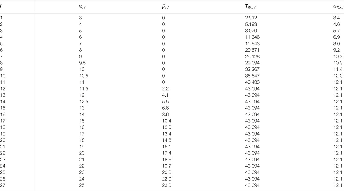
TABLE A1. States of the i steady state operations points OP_i of the NREL FAST 5MW reference wind turbine with the wind speed v_c,i, rotor rotational speed ${\omega }_{\mathcal{R},c,i}$, generator torque T_G,c,i and pitch angle β_c,i.

TABLE A2

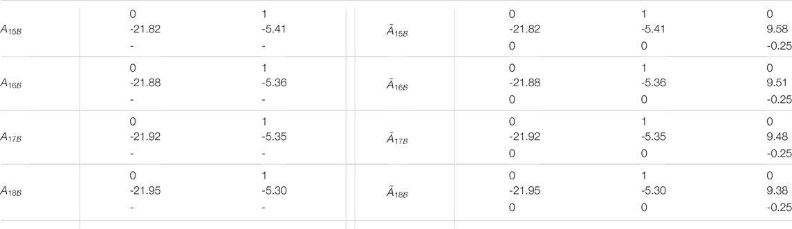
TABLE A2. State matrices $A_{i\mathcal{B}}$ and augmented state matrices ${\tilde{A}}_{i\mathcal{B}}$ of the $\mathcal{B}$lade model (for the submodels i ∈ [15,18]).

TABLE A3

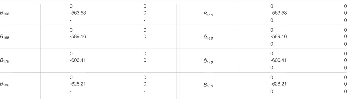
TABLE A3. Input matrices $B_{i\mathcal{B}}$ and augmented input matrices ${\tilde{B}}_{i\mathcal{B}}$ of the $\mathcal{B}$lade model (for the submodels i ∈ [15,18]).

TABLE A4

TABLE A4. Common output matrix $C_{\mathcal{B}}$ and augmented common output matrix ${\tilde{C}}_{\mathcal{B}}$ of the $\mathcal{B}$lade model (for all submodels).

TABLE A5

TABLE A5. Steady states ${\underline{x}}_{c,i\mathcal{B}}$ and augmented steady states ${\underline{\tilde{x}}}_{c,i\mathcal{B}}$ of the $\mathcal{B}$lade model (for the submodels i ∈ [15,18]).

TABLE A6

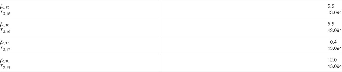
TABLE A6. Steady state pitch angle β_c,i and generator torque T_G,i (for the submodels i ∈ [15,18]).

TABLE A7

TABLE A7. State feedback matrices $K_{i\mathcal{R}}$ of the (rigid body) $\mathcal{R}$otion drive train model (for the submodels i ∈ [15,18]).

TABLE A8

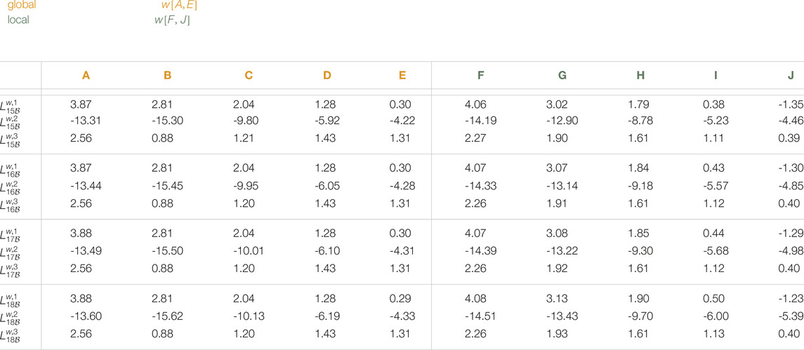
TABLE A8. Error state feedback gain matrices $L_{i\mathcal{B}}^{w,j}$ of the blade model based wind speed observers $\mathcal{B}$ for:- $\text{global}$ Lyapunov approach with $w\in \left[A,,,E\right]$- $\text{local}$ Lyapunov approach with $w\in \left[F,,,J\right]$- submodels i ∈ [15,18]- matrix elements j ∈ [1,3].

TABLE A9

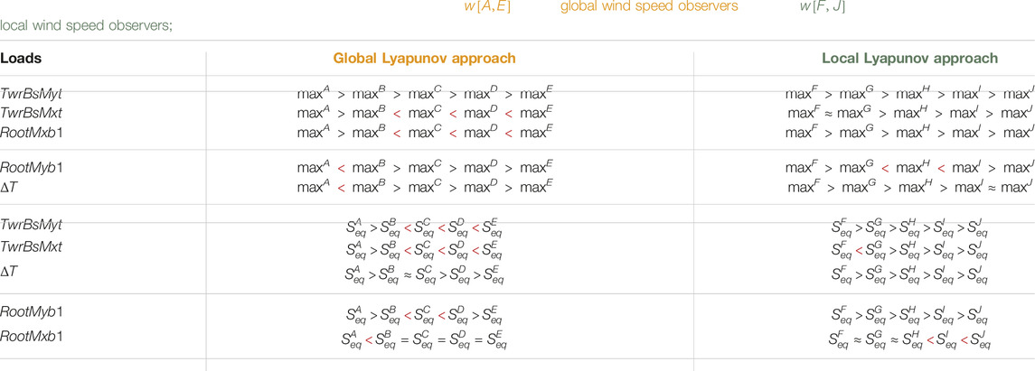
TABLE A9. Analysis of the ultimate loads max^w and fatigue loads $S_{eq}^w$ resulting from five different wind speed observers regarding the steady increase or decrease of the loads (evaluated separately for each of the two Lyapunov approaches with $w\in \left[A,,,E\right]$ for the $\text{global wind speed observers}$ and with $w\in \left[F,,,J\right]$ for the $\text{local wind speed observers;}$ based on the loads depicted in Figure 8).

TABLE A10

TABLE A10. Analysis of the ultimate loads max^w and fatigue loads $S_{eq}^w$ resulting from five different wind speed observers regarding the steady increase or decrease of the loads (comparing both Lyapunov approaches with each other with $w\in \left[A,,,E\right]$ for the $\text{global wind speed observers}$ and with $w\in \left[F,,,J\right]$ for the $\text{local wind speed observers;}$ based on the loads depicted in Figure 8).

All states and parameters are expressed in SI units, despite the generator torque T_G (that is expressd in kNm), pitch angles (that are expressed in (angular) degree) and the rotation speed (expressed in revolution per minute).

Specification of the LMI constraints

Restrictions for the decay rates α_{min  / max} and natural frequencies of the system response (characterised by the real part and imaginary part of the closed-loop poles Re(s_P,i) and Im(s_P,i)) can be specified with bounds, e.g. with horizontal lines (with α_max < Re(s_P,i) < α_min)) and diagonal origin lines (with $\text{tan}(\theta )<\frac{\text{Im}(s_{P,i})}{\text{Re}(s_{P,i})}\iff \theta <\text{arctan}\frac{\text{Im}(s_{P,i})}{\text{Re}(s_{P,i})}$, also denoted as cone angle) in the complex pole map, resulting in bounded pole map segments and pole regions, respectively (Pöschke et al., 2019).

In (Chilali and Pascal, 1996), LMI representations for these bounded pole map segments, i.e. the restricted location of the poles and eigenvalues of a linear system, respectively, are derived.

For the upper vertical bound ${\alpha }_{\mathcal{B},\max }$ of the error dynamics, based on the blade design model, the following LMI holds (with $N_i^w=P_i^w{L}_{i\mathcal{B}}^w$, defined in (20)):

$A_{i\mathcal{B}}^T{P}_i-C_{\mathcal{B}}^T{N}_i^{w^T}+P_i{A}_{i\mathcal{B}}-N_i^w{C}_{\mathcal{B}}\succ -2{\alpha }_{\mathcal{B},\max }{P}_i,(23)$

and for the lower vertical bound ${\alpha }_{\mathcal{B},\min }$ it holds:

$A_{i\mathcal{B}}^T{P}_i-C_{\mathcal{B}}^T{N}_i^{w^T}+P_i{A}_{i\mathcal{B}}-N_i^w{C}_{\mathcal{B}}\prec -2{\alpha }_{\mathcal{B},\min }{P}_i.(24)$

For the cone angle bound θ of the error dynamics, based on the blade design model, the following LMI holds:

$\left[\begin{array}{c}\hfill \sin \left(\theta \right)\left(-A_{i\mathcal{B}}^T{P}_i-C_{\mathcal{B}}^T{N}_i^{w^T}+P_i{A}_{i\mathcal{B}}-N_i^w{C}_{\mathcal{B}}\right)\hfill \\ \hfill \text{cos}\left(\theta \right)\left(-A_{i\mathcal{B}}^T{P}_i+C_{\mathcal{B}}^T{N}_i^{w^T}+P_i{A}_{i\mathcal{B}}-N_i^w{C}_{\mathcal{B}}\right)\hfill \\ \hfill \text{cos}\left(\theta \right)\left(-A_{i\mathcal{B}}^T{P}_i-C_{\mathcal{B}}^T{N}_i^{w^T}-P_i{A}_{i\mathcal{B}}+N_i^w{C}_{\mathcal{B}}\right)\hfill \\ \hfill \sin \left(\theta \right)\left(-A_{i\mathcal{B}}^T{P}_i-C_{\mathcal{B}}^T{N}_i^{w^T}+P_i{A}_{i\mathcal{B}}-N_i^w{C}_{\mathcal{B}}\right)\hfill \end{array}\right]\prec 0.(25)$

The matrices used in (23) to (25) are listed in Tables A2, A4, A8.

All simulations were executed with the controller ct1210013. The following global Lyapunov approach based wind speed observers were used: A ≡ ot1210027, B ≡ ot1210030, C ≡ ot1210033, D ≡ ot1210051, E ≡ ot1210049, F ≡ ot1210036, G ≡ ot1210039, H ≡ ot1210042, I ≡ ot1210043, J ≡ ot1210044.

The state observer ot1010001 was utilised.

For the wind excitation the Imp14.hh wind time series is used.

To calculate the mean Euclidian norm ${\Vert L_{i\mathcal{B}}^{w,\overline{j}}\Vert }_2$ of the error-feedback gains $L_{i\mathcal{B}}^{w,j}$ [see (26)] and the average, mean Euclidian norm ${\Vert L_{\overline{i}\mathcal{B}}^{w,\overline{j}}\Vert }_2$ [see (27)] the worksheet Uebersicht_L_Matrizen_Pitchwinkel-YYYY_MM_DD.xlsx is used.

Load analysis

For the ultimate loads $ma{x}^w$ and fatigue loads $S_{eq}^w$, resulting from five different wind speed observers (i.e. for the $w\in \left[A,,,E\right]$ $\text{global}\hspace{0.17em}\text{wind speed observers}$ and $w\in \left[A,,,E\right]$ $\text{local wind speed observers}$; see Figure 8), the steady increase or decrease of the loads is evaluated separately for each of the two observer approaches (see Table A9) and in comparison to each other (see Table A10).