Evaluation of the ocean component on different coupled hurricane forecasting models using upper-ocean metrics relevant to air-sea heat fluxes during Hurricane Dorian (2019)

1 Introduction

In the last three decades there has been a 50%–70% reduction in the forecast error of the storm track in operational Atlantic hurricane models (https://www.nhc.noaa.gov/verification/verify5.shtml). On the other hand, the error reduction in the intensity forecast has been marginal, particularly for short (24–48 h) lead forecast times (https://www.nhc.noaa.gov/verification/verify5.shtml). There are several reasons why tropical cyclone intensity forecasting has remained a challenge. This includes inaccuracies in ocean initial conditions and the difficulty of correctly representing the upper-ocean mass properties and processes that feedback into the hurricane through air-sea heat and momentum fluxes in coupled atmosphere-ocean models (Chen et al., 2007; Zhang et al., 2008; Halliwell et al., 2011; Jaimes et al., 2011).

The classical theory of tropical cyclones establishes that the intensity of a storm, measured as the minimum central surface pressure, is the result of the balance between the air-sea enthalpy fluxes, energy loss due to frictional dissipation, and heat loss to the surroundings (Emanuel, 1986). It is then clear that both the atmospheric conditions as well as the oceanic conditions are important in the genesis, development, and intensity changes of tropical cyclones. In particular, it has been shown that the upper-ocean thermal (Emanuel, 1999; Shay et al., 2000) and salinity structures (Balaguru et al., 2012, 2020; Domingues et al., 2015; Dong et al., 2017) play a key role in the intensification of tropical cyclones. For example, it has been reported that a number of tropical cyclones intensify when they travel over warm ocean features (Leipper and Volgenau, 1972; Shay et al., 2000; Lin et al., 2009; Le Hénaff et al., 2021) or over low salinity barrier layers (Domingues et al., 2015), and that a reduced sea surface temperature cooling of the ocean area under the storm inner-core is linked to storm intensification (Cione and Uhlhorn, 2003).

Since 2011 the National Oceanic and Atmospheric Administration, with the participation of other government, academic, and private industry partners, is leading efforts to conduct ocean observations from an array of underwater gliders in support of hurricane research and forecast, in areas of the North Atlantic Ocean, tropical Atlantic Ocean, the Gulf of Mexico, and the Caribbean Sea, where tropical storms form and evolve (e.g., Glenn et al., 2016; Miles et al., 2017, 2021; Domingues et al., 2019). These efforts are complemented by the already in place components of the sustained ocean observing system and of targeted observations dedicated specifically to tropical cyclone research. The use of data from these sustained and targeted observations has been shown to reduce the error in intensity forecasts within various experimental and operational schemes and models (Mainelli et al., 2008; Dong et al., 2017; LeHenaff et al., 2021).

On 19 August 2019, Hurricane Dorian developed from a tropical wave off the west coast of Africa and moved through the Caribbean Sea gaining strength. On 28th August, it transitioned from a tropical storm to a category 1 hurricane. Around this date, the path of Dorian moved through a glider array (Figure 1) operated by the NOAA Atlantic Oceanographic and Meteorological Laboratory (AOML) and the Caribbean Regional Association of the integrated Ocean Observing System (CARICOOS), in the Caribbean Sea off Puerto Rico and the U.S. Virgin Islands. After traveling through this glider array, Dorian continued moving northwestward and made landfall in Great Abaco Island (Bahamas) on September 1st as a category 5 hurricane, becoming the strongest hurricane on record to make landfall in the Bahamas. None of the operational hurricane forecast models captured the correct intensity evolution during the 5 days prior to Dorian reaching its maximum strength (Avila et al., 2020).

Figure 1

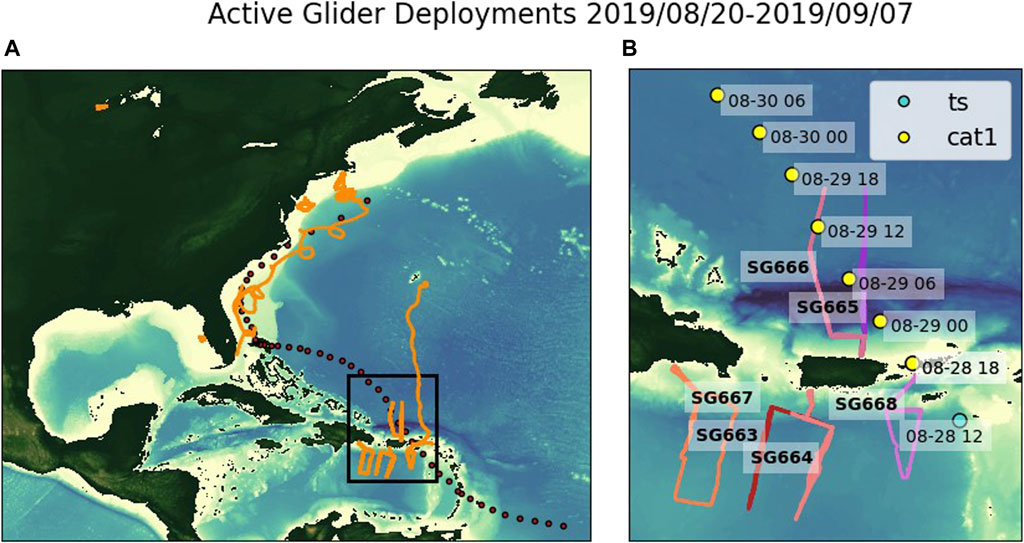
Figure 1. (A) North Atlantic map showing the path of hurricane Dorian (red dots) and the glider trajectories between 20 August and 7 September 2019 (orange lines). (B) Zoom in on the black rectangle in (A) showing the path and category (circles) of Hurricane Dorian and the glider trajectories.

The goal of this manuscript is to present an assessment of how different initialization strategies used in coupled atmosphere-ocean hurricane models affected the representation of upper-ocean thermal fields that are key for air-sea heat fluxes during Hurricane Dorian. In order to accomplish this, we evaluated the upper-ocean thermal structure simulated by three NOAA coupled atmosphere-ocean hurricane models during the approach of Dorian to the Bahamas. The data set used here contains 587 temperature and salinity profiles from the array of underwater gliders present south of Puerto Rico from August 28 00 UTC to September 02 06 UTC, 2019. We also evaluated the data-assimilative Navy operational Global Ocean Forecasting System (GOFS 3.1) in order to provide a baseline for the skill of several ocean metrics from a data-assimilative model as compared to the free-running ocean component of the hurricane forecasting models.

As part of the work, we assessed four upper-ocean metrics that have been previously identified as being linked to the intensification of tropical storms. The first two metrics are the mean temperature and mean salinity within the surface mixed layer. The surface mixed layer is the surface portion of the water column where turbulent processes, such as wind-driven mixing, make water density nearly uniform (de Ruijter, 1983). The disequilibrium between the air surface temperature and the sea surface temperature, estimated here as the mixed layer temperature, controls the magnitude and direction of the air-sea sensible and latent heat fluxes (Malkus and Riehl, 1960; Emanuel, 1986). The mixed layer salinity is important since a low salinity mixed layer is often associated with the presence of salinity-induced barrier layers. Barrier layers form when a surface layer of fresh water dominates the upper layer density structure over temperature changes, so that the depth of the isothermal layer (the layer of quasi-constant temperature at the ocean surface) and the depth of the mixed layer (the layer of quasi-constant density at the ocean surface) differ. Barrier layers are often observed in the eastern Caribbean Sea, portions of the Tropical Atlantic, and in the northern Gulf of Mexico. The surface layer of low salinity waters in the Caribbean Sea and adjacent portions of the Tropical Atlantic is the result of the spreading of the Amazon and/or Orinoco river plumes (Hu et al., 2004). Data retrieved from the Optimally Interpolated Sea Surface Salinity Global Dataset V2 (https://podaac.jpl.nasa.gov/dataset/OISSS_L4_multimission_7day_v2) shows that during the passage of Hurricane Dorian through the Caribbean, the influence of the Amazon/Orinoco river plumes extended north, affecting the sea surface salinity south and north of Puerto Rico, with average salinity values of 34.5 and 35.5, respectively. Similarly, barrier layers in the northern Gulf of Mexico are created by the outflow of fresh waters from the Mississippi river. There is evidence that when storms travel over barrier layers, these layers can promote the intensification of tropical cyclones by enhancing the vertical stability of the water column and, therefore, reducing the storm-induced vertical mixing (Balaguru et al., 2012, 2020; Domingues et al., 2015; Rudzin et al., 2019). The third metric analyzed in this work is the ocean heat content (OHC), defined as the excess of heat in the surface ocean above the 26 degrees isotherm (Whitaker, 1967; Leipper and Volgenau, 1972). The OHC or Tropical Cyclone Heat Potential (TCHP) is a metric that has been shown to be correlated with the intensification of major hurricanes in the Atlantic Ocean (Mainelli et al., 2008). The fourth metric is the depth-averaged temperature in the top 100 m (T100). T100 was proposed as a metric that quantifies the resulting sea surface temperature after the passage of a hurricane that fully mixes the top 100 m, accounting for the effect of cold subsurface water and the strength of vertical mixing on storm weakening (Price, 2009).

This manuscript is organized as follows. The glider observations and the hurricane forecasting models used here are described in Section 2. The results of the model evaluation are reported in Section 3. The implications and conclusions of our results for coupled atmosphere-ocean models are presented in Section 4.

2 Methods

2.1 Observational data sources

A fleet of 54 underwater gliders was deployed in the Caribbean Sea and tropical Atlantic, Gulf of Mexico, the South and Mid-Atlantic Bight during the 2019 hurricane season as part of a U.S. government, academic, and private industry wide effort to carry out ocean observations in support of Atlantic hurricane research and forecasts (Miles et al., 2021). Underwater gliders are autonomous vehicles that use variable buoyancy to travel in a sawtooth-like profile and are equipped to collect a variety of ocean variables. This effort complemented other observations carried out by profiling floats, surface drifters, eXpendable BathyThermographs (XBTs), moorings, and other observational platforms. During the passage of Hurricane Dorian through the Caribbean region, six gliders operated by the NOAA/AOML and the CARIbbean Coastal Ocean Observing System (CARICOOS), collected temperature and salinity profiles along fixed predetermined transects to 500 m depth with an approximate repeat interval of 2 h (Figure 1). The data from these six gliders are used in this study as the main observational asset to evaluate the coupled models outputs.

2.2 Numerical data sources

We first evaluated the US Navy Global Ocean Forecasting System (GOFS 3.1) (Metzger et al., 2017). GOFS 3.1 is based on the HYbrid Coordinate Ocean Mode (HYCOM) coupled with the Los Alamos Sea Ice Code (CICEv4) with a 3-dimensional variational (3DVar) data assimilation algorithm implemented in the Navy Coupled Ocean Data Assimilation (NCODA). GOFS3.1 has 41 hybrid vertical layers and a horizontal resolution of 0.08 of a degree in latitude and longitude between 40 degrees South and 40 degrees North. Poleward of 40 degrees North/South, the grid has a resolution of 0.08 degrees in longitude and 0.04 in latitude. It is forced by the US Navy Global Environmental Model (NAVGEM; Hogan et al., 2014). NCODA assimilates satellite altimeter data, satellite and in situ sea surface temperature, in situ vertical temperature and salinity from Argo floats, buoys, gliders, and XBTs (temperature only). Details about the GOFS 3.1/NCODA system can be found in the GOFS 3.1 validation test report (Metzger et al., 2017). The hindcast output for GOFS 3.1 used here can be accessed at https://tds.hycom.org/thredds/dodsC/GLBv0.08/expt93.0/ts3z.html.

In addition, three coupled atmosphere-ocean hurricane forecast models were evaluated in this work:

(1) The Hurricane Weather and Forecasting model (HWRF) coupled to the Message Passing Interface Princeton Ocean Model—Tropical Cyclone (MPIPOM-TC), which was until 2022 one of the operational hurricane forecasting systems ran by NOAA National Centers for Environmental Prediction (NCEP) (Biswas et al., 2018). Hereafter, we will call this coupled system HWRF2019-POM. The MPIPOM-TC of HWRF2019-POM was initialized from the Generalized Digital Environmental Model (GDEM) monthly ocean temperature and salinity climatology (Carnes, 2009; Teague et al., 1990) and a feature-based modeling procedure (Yablonski and Ginis, 2008), to sharpen thermal fronts using information of remote sensed sea surface temperature and the Naval Oceanographic Office (NAVO) frontal analysis (Rhodes et al., 2001). The atmospheric component of HWRF2019-POM used initial and boundary conditions from the Global Forecasting System (GFS) v15.1 (GDAS/GFS v15.0.0, 2018). For this configuration, MPIPOM-TC contains 40 terrain-following vertical levels, with a vertical resolution that ranges between 2 and 20 m in the top 100 m of the water column. For the North Atlantic domain, the grid extends from 7.5 to 45.0 degrees North and from −98.5 to −15.3 degrees West, with a uniform horizontal resolution of 9.2 km in latitude and 10.5 in longitude. The vertical mixing parameterization used in the upper ocean mixed layer is Mellor-Yamada 2.5 turbulence closure model (Mellor and Yamada, 1982).

(2) An experimental coupled model, HWRF2020-POM, with the same ocean component, vertical and horizontal resolution, and model physics as HWRF2019-POM but initialized from the HYCOM-based NOAA’s Real Time Ocean Forecasting System (RTOFS) (Garraffo et al., 2020). During the 2019 hurricane season, RTOFS was initialized daily from GOFS 3.1. But since December 2020, it has used its own flow-dependent 3DVar data-assimilative system with quality control, variational analysis and diagnostics. This system was originally based on the Navy Coupled Data Assimilation System (Cummings and Smedstad, 2013), and includes assimilation of ADT SSH, satellite SST, satellite SSS, satellite ice coverage, in situ SST, SSS, and profiles.

(3) An experimental system, HWRF coupled to HYCOM, HWRF2020-HYCOM, was also initialized from RTOFS (Kim et al., 2014, 2022). The difference from HWRF2020-POM is the model configuration, subgrid mixing physics and a set of feedback forcing variables (Biswas et al., 2018). HYCOM uses the same model configuration as the global RTOFS. In the open ocean, the vertical coordinate is isopycnal and transitions to z-levels in the weakly stratified upper-ocean mixed layer. In shallow waters, the vertical coordinate is terrain-following sigma and transitions to z-levels in the upper mixed layer. In the configuration used, HYCOM has 41 hybrid vertical layers, with a vertical resolution ranging between 2 and 20 m in the top 100 m of the water column. For the North Atlantic domain, the grid extends from 1 to 45.7 degrees North and from −98.2 to −7.5 degrees West. The horizontal resolution is of approximately 9 km in longitude and ranges from 8.7 km to 6.1 km in latitude. HYCOM supports several vertical mixing schemes. This configuration used the K profile parameterization (KPP) (Large et al., 1994).

The models used in this analysis are summarized in Table 1.

2.3 Upper-ocean metrics

In this study we considered four upper-ocean metrics: mixed layer temperature, mixed layer salinity, ocean heat content, and average temperature in the upper 100 m.

Table 1

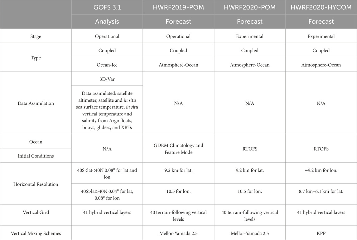
Table 1. Summary of numerical models.

The mixed layer depth (MLD) was estimated as the surface portion of the water column within which changes of hydrographic characteristics are smaller than a threshold value. We used two definitions of the MLD, one based on a temperature criteria with the threshold value of 0.2°C (Eq. 1), and the other based on a density criteria with a threshold value 0.125 kg m⁻³ (Eq. 2) (de Boyer Montégut et al., 2004).

$\mathrm{T}-{\mathrm{T}}_{10}\le {0.2}^{\mathrm{o}}\mathrm{C}(1)$

${\mathrm{\rho }}_{10}-\mathrm{\rho }\le 0.125\text{kg}{\mathrm{m}}^{-3}(2)$

Where T₁₀ and ρ₁₀ are the water temperature and density at 10 m depth, respectively. The choice of 10 m as a reference depth does not affect the estimates of the mixed layer depth because this depth is always within the low salinity layer that is often found at the ocean surface in the study area. In general, there is no guarantee that the temperature and density criteria cannot be satisfied for depths deeper than the MLD. However, in our study area of the 587 density profiles analyzed, the density criteria was never satisfied below the MLD, implying that density was monotonically increasing with depth. The average temperature and salinity within the mixed layer are calculated as the average temperature and salinity of the portion of the vertical profile that is within the mixed layer.

The Ocean Heat Content (OHC) is defined as the depth-integrated excess above 26°C between the sea surface and the depth of the 26°C isotherm (Z26) (Whitaker, 1967; Leipper and Volgenau, 1972):

$\text{OHC}={\mathrm{C}}_{\mathrm{p}}{\mathrm{\rho }}_0{\int }_{z26}^0\left(T\left(z\right)-26\right)dz,forT\left(z\right)>26(3)$

Where C_p is the heat capacity of sea water, ρ₀ is the mean density of the water column down to Z26, and T(z) is temperature at different depths in degrees Celsius.

The depth-averaged temperature in the top 100 m (T100) is a metric that estimates the potential resulting SST after the passage of a hurricane due to vertical mixing processes. A depth of 100 m is chosen as a typical depth of complete vertical mixing under a category 3 hurricane (Price, 2009; Domingues et al., 2015). This metric is particularly informative in waters where the OHC cannot be estimated, i.e., for temperatures lower than 26°C, but still provides information on the subsurface temperature structure. However, in regions where salinity significantly contributes to the vertical stratification of the upper water column, e.g., regions with barrier layers, T100 may not be a good approximation for the resulting SST due to the storm-induced vertical mixing. In this case, a more general metric should be used where the depth over which the temperature is averaged, depends on the assumption that the bulk Richardson number of the surface mixed layer is less than 0.6 (Price, 2009).

2.4 Taylor diagrams and bias

In order to quantify the skill of the four models in reproducing the upper-ocean thermal structure, we estimated the normalized standard deviation and correlation between the observational and the model data. We used all the available temperature and salinity profiles from the six gliders located north and south of Puerto Rico when Hurricane Dorian was transiting through that region, from 28 August to 2 September 2019 (Figure 1). In order to conduct these comparisons, we found the corresponding grid points and timestamps in the different models for the observed temperature and salinity profiles, by linearly interpolating in space and time the measurement locations and times onto the model’s grids and times. For the hurricane forecasting models, we used the forecasting cycle 2019082800 that started at 00 UTC on 28 August, and included the time when Hurricane Dorian transitioned from a Tropical Storm to a Category 1 hurricane as it was passing through the glider array. We want to point out that, because of a 2-day latency between the last data assimilation and the state estimate in the RTOFS system used in 2019, the ocean estimates from RTOFS, which are used in the HWRF2020-POM and the HWRF2020-HYCOM products, do not include observations past August 26 00 UTC in the considered cycle. This means that the coupled models were not fed with recent observations at the time of the passage of the hurricane. For GOFS 3.1, we used the aggregated analysis time series, which includes data assimilation throughout the study period.

The normalized standard deviation and correlation for all the different metrics can be visualized together by constructing a Taylor diagram (Taylor, 2001), giving us a compact way to assess the skill of each coupled atmosphere-ocean hurricane forecast model. The bias and the bias percentage are:

$\text{Bias}=\text{Xmodel}-\text{Xobs},\text{and}(4)$

$\text{Bias}\%=\left(\text{Xmodel}-\text{Xobs}\right)/\text{Xobs}\times 100\%(5)$

Where Xobs is the observed mean value of a specific metric and Xmodel is the mean value of the same metric obtained from the outputs of the various models.

2.5 Cross track radius and sea surface heat loss per unit area

The cross track radius (r) of a geographical point at a specific time is defined as the distance from the center of the storm to that specific point. The normalized cross track radius is defined as the cross track radius divided by the radius of maximum winds (Rmax).

The sea surface heat loss per unit area (SSHL), is defined as the enthalpy flux, i.e., the sum of the sensible and latent heat flux, integrated over time (Shay and Uhlhorn, 2008; Jaimes et al., 2015), Eq. 6,

$\text{SSHL}\left(\mathrm{r}/\text{Rmax}\right)={\int }_{to}^{T}Q\left(t\right)dt(6)$

where Q represents the enthalpy flux and dt is the time interval that the storm travels along the storm path. Since we are using the HWRF output to estimate SSHL, dt is equal to 3 h, which is the time interval between consecutive model outputs.

3 Results

3.1 Model evaluation

The temperature transects from the glider observations show that the surface temperatures in the tropical Atlantic Ocean just north of Puerto Rico at the end of August were close to 30°C and that the Z26 was approximately at 100 m depth (Figure 2A). A qualitative comparison of the temperature field between the glider transect SG665, GOFS 3.1, and the three coupled hurricane forecast models (forecast cycle 2019082800) from 28 August to 2 September 2019, shows that Z26 is approximately 100 m in the observations, and around 10 m shallower for all the models (Figures 2B–E).

Figure 2

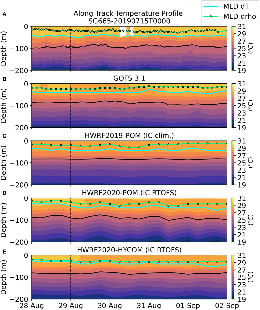
Figure 2. (A) Temperature transect for glider SG665 from 29 August to 2 September. (B–E) The same along-track transect as for SG665 but interpolated onto the respective model grid and timestamp. The cyan and green lines show the mixed layer depths based on the temperature criteria (Eq. 1, “MLD dT” in the legend) and the density criteria (Eq. 2, “MLD drho” in the legend), respectively. The black contour in figures (A–E) shows the 26°C isotherm. The dashed vertical line in all figures shows the time when Hurricane Dorian was the closest to glider SG665. For this figure we used the forecast cycle 2019082800 for the hurricane forecasting models and the aggregated analysis time series for GOFS 3.1.

The glider observations also show that the MLD based on the temperature criteria (Eq. 1) is about 25 m deeper than the MLD based on the density criteria (Eq. 2) (Figures 2–4). Overall, all four models exhibit the same pattern of a deeper MLD based on the temperature criteria, although the MLDs differ from the value obtained from the observations, and among the models. For example, the mean value from 28 August to 2 September 2019 of the MLD based on the density criteria is: 20.5 m for the glider observations, 19.3 m for GOFS 3.1, 18.4 m for HWRF2019-POM, 24.4 m for HWRF2020-POM, and 27.9 m for HWRF2020-HYCOM. Therefore, the current operational models appear limited in their capacity to represent and, consequently, predict the mixed layer thickness and its evolution.

Figure 3

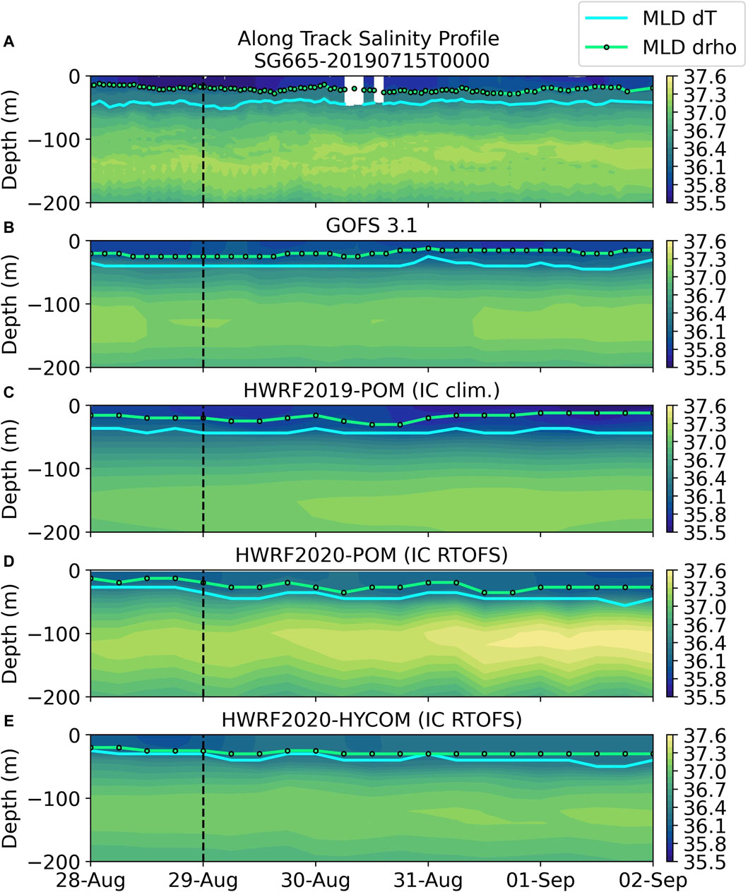
Figure 3. (A) Salinity transect for glider SG665 from August 29 to September 2. (B–E) The same along-track transect as for SG665 but interpolated onto the respective model grid and timestamp. The blue and green lines show the mixed layer depths based on the temperature criteria (Eq. 1, “MLD dT” in the legend) and the density criteria (Eq. 2, “MLD drho” in the legend). The dashed vertical line in all figures shows the time when Hurricane Dorian was the closest to glider SG665. For this figure we used the forecast cycle 2019082800 for the hurricane forecasting models and the aggregated analysis time series for GOFS 3.1.

Figure 4

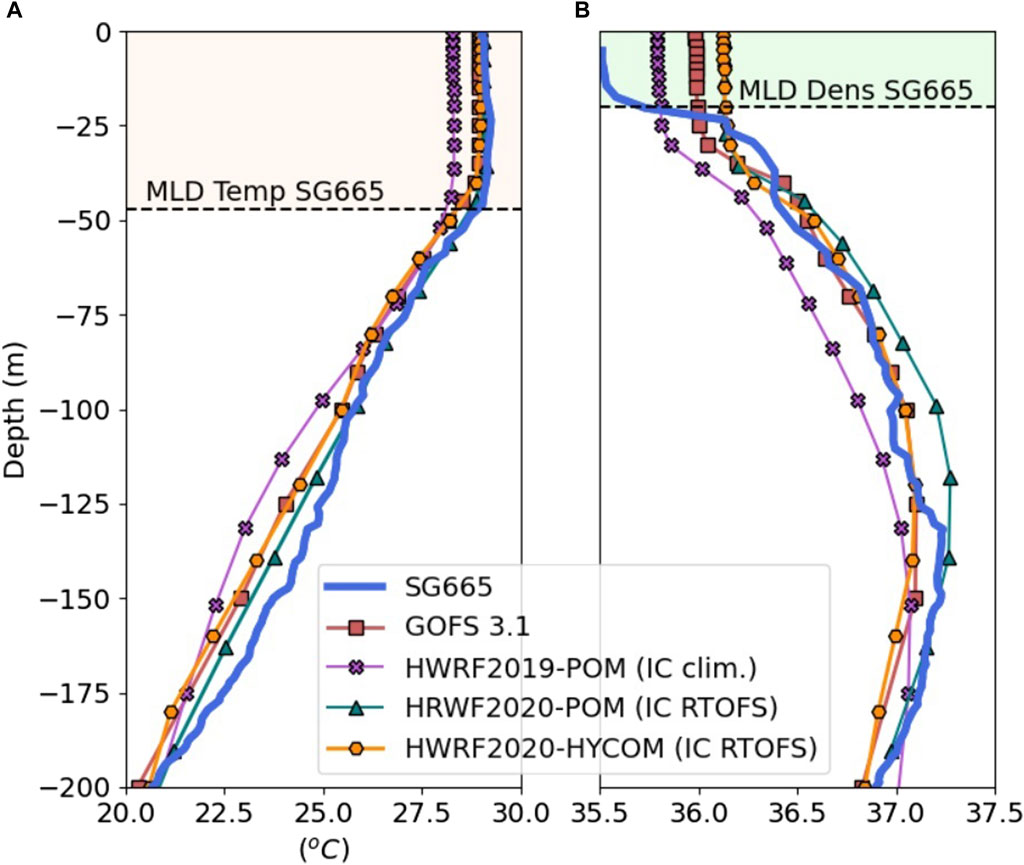
Figure 4. Vertical profiles of (A) temperature, and (B) salinity, for glider SG665 (blue), GOFS 3.1 (red), HWRF2019-POM (IC clim.) (purple), HWRF2020-POM (IC RTOFS) (green) and HWRF2020-HYCOM (IC RTOFS) (orange) at the time when Hurricane Dorian was the closest to glider SG665. For this figure we used the forecast cycle 2019082800 for the hurricane forecasting models and the aggregated analysis time series for GOFS 3.1. The dashed lines show the mixed layer depth based on (A) the temperature criteria and on (B) the density criteria, in both for glider SG665.

The difference in the MLD estimates using the two different criteria is caused by the presence of barrier layers. During the passage of Hurricane Dorian close to the glider array, there was a barrier layer north of Puerto Rico, with surface salinity values of 35.5, consistent with the data retrieved from the Optimally Interpolated Sea Surface Salinity Global Dataset V2, as it is shown in the salinity transect from glider SG665 (Figure 3A) and salinity vertical profile (Figure 4B). As a consequence, salinity rather than temperature controlled the vertical stratification at the surface in that portion of the Tropical Atlantic. For this reason, we will use the estimate of the surface mixed layer depth based on the density criteria from now on in our analysis.

Despite the general agreement in the Z26, there are differences of about 0.9°C to 0.1°C between the observed and the model-derived mixed layer temperature (MLT) (Figure 5A). HWRF2019-POM, initialized from climatology, is ∼1°C colder than observations. HWRF2020-POM and HWRF 2020- HYCOM, both initialized from RTOFS, have a similar temperature of 29.3°C as the observations during the first 24 h, but beyond this point the mixed layer temperature gets progressively colder. GOFS 3.1, the data assimilative model, starts colder than the glider temperature but it approaches the observed temperature values at 12Z on August 30.

Figure 5

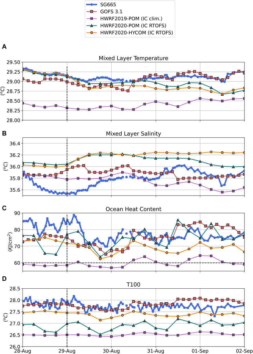
Figure 5. Time series of (A) mixed layer temperature (MLT), (B) mixed layer salinity, (C) ocean heat content (OHC) and (D) depth-averaged temperature in the top 100 m (T100) for glider SG665 (blue), GOFS 3.1 (red), HWRF2019-POM (IC clim.) (purple), HWRF2020-POM (IC RTOFS) (green) and HWRF2020-HYCOM (IC RTOFS) (orange). The dashed vertical line in all figures shows the time when Hurricane Dorian was the closest to glider SG665. For this figure we used the forecast cycle 2019082800 for the hurricane forecasting models and the aggregated analysis time series for GOFS 3.1.

The time series of the mixed layer salinity (Figure 5B) shows that around the time of the passage of Hurricane Dorian through the glider array, none of the models captured the lower salinity that characterized the surface layer at that time. Additionally, the vertical structure of salinity in the different models has a surface layer of low salinity that is deeper and less sharp than the observations reveal. The first key result shown here is that the models failed to capture the upper-ocean salinity values and the vertical structure of the associated barrier layer during this period (Figures 3B–E, 4B, 5B).

Before the passage of Dorian, the OHC observed by the glider SG665 (located north of Puerto Rico) is ∼85 kJ cm⁻², well above 60 kJ cm⁻² (Figure 5C), which is a statistically-determined threshold shown to favor storm intensification in the Atlantic (Mainelli et al., 2008). The OHC in HWRF2019-POM during that same time-frame is ∼60 kJ cm⁻², which is well below the observed value. The other models exhibit an OHC closer to the measured OHC, although HWRF2020-HYCOM is consistently lower than the glider estimate. In agreement with the results for the OHC, T100 from HWRF2019-POM is the lowest of all the models, while GOFS3.1 exhibits values between 27.8°C and 28.1°C, being closer to the observations (Figure 5D).

We obtained the skill of the models by obtaining the normalized Taylor diagram and calculating the bias between the glider observations and the different models. The normalized Taylor diagram shows that all the models have a good skill in the temperature (Temp) and salinity (Salt) averaged over the entire observed water column, i.e., down to 500 m (Figure 6A). However, the models’ skill substantially decreases for the upper-ocean metrics. A second key result is that the four metrics relevant for the air-sea heat fluxes: mixed layer temperature (MLT), mixed layer salinity (MLS), ocean heat content (OHC) and depth average temperature in the top 100 m (T100), are not well represented in the different models. In particular, HWRF2019-POM, initialized from climatology has the lowest skill for the upper-ocean metrics (Figure 6B), while HWRF2020-HYCOM, initialized from RTOFS, and GOFS 3.1, the data assimilative model, have the highest skill for the same metrics.

Figure 6

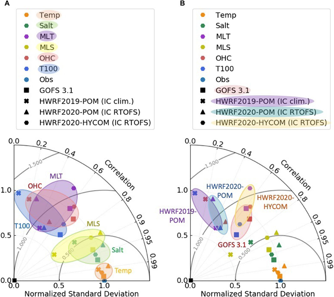
Figure 6. Normalized Taylor diagram showing the skill of the four models evaluated: GOFS 3.1, HWRF2019-POM (IC clim.), HWRF2020-POM (IC RTOFS) and HWRF2020-HYCOM (IC RTOFS). In (A) the skill is grouped by different quantities, namely, temperature (Temp) and salinity (Salt) over the full depth covered by the glider profiles, mixed layer temperature (MLT) and mixed layer salinity (MLS) using the density criteria (Eq. 2), ocean heat content (OHC) (Eq. 3) and depth average temperature in the top 100 m (T100). In (B) the skills for the three thermal upper-ocean metrics, i.e., MLT, OHC, and T100, are grouped according to the different models. For this figure we used the forecast cycle 2019082800 for the hurricane forecasting models and the aggregated analysis time series for GOFS 3.1 from 28 August to 2 September 2019.

The bias (Table 2) for the MLT shows that all the models are colder than observations within the ocean surface mixed layer, with HWRF2019-POM initialized from climatology being the coldest. We see a similar pattern for the OHC. HWRF2019-POM presents a 22% (−18.8 kJ cm⁻²) deficit in OHC with respect to the observations, while data assimilative model GOFS 3.1 has only a deficit of 3.6% (−3.1 kJ cm⁻²). Among the coupled hurricane forecast models, HWRF2020-HYCOM has the lowest MLT and OHC bias. The bias for the MLS shows that all the models tend to predict higher salinity values in the mixed layer. A key third result obtained here is that the model with the lowest MLS is GOFS 3.1, demonstrating the benefits of ocean data assimilation to correct the biases not only in temperature but also in salinity.

Table 2

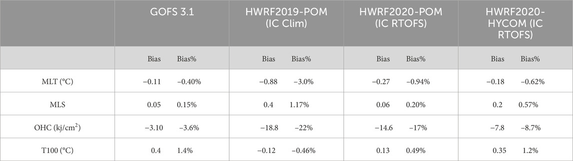
Table 2. Bias (Eq. 4) and bias percentage (Eq. 5) between the observations and the different models for the mixed layer temperature (MLT), mixed layer salinity (MLS), ocean heat content (OHC) and depth average temperature in the top 100 m (T100).

3.2 Mixed layer temperature and sea surface heat loss

We estimated the mixed layer temperature (MLT) and sea surface heat loss (SSHL) at three different times along Dorian’s forecasted track (Figure 7): At 18 h forecast lead time, T1, Dorian’s intensity is close to category 1 in all models, At 66 h lead time, T2, the intensity of the different models differ by at least 1 category, and at 84 h lead time, T3, all the models are predicting approximately a category 4 hurricane.

Figure 7

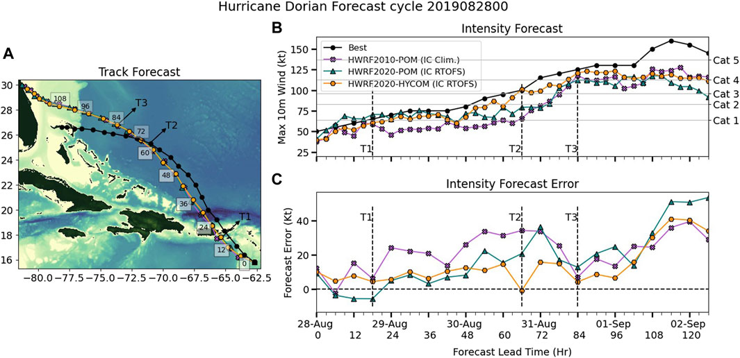
Figure 7. (A) Best track (black line) and Forecasted tracks, (B) observed (black line) and forecast intensity, and (C) Absolute relative intensity error for the three coupled hurricane forecasting models evaluated: HWRF2019-POM (IC Clim.) in purple, HWRF2020-POM (IC RTOFS) in green, and HWRF2020-HYCOM (IC RTOFS) in yellow. The forecast cycle used here is cycle 2019082800. The forecasted lead times highlighted in the figures are the 18 h (T1), 66 h (T2), and the 84 h (T3) lead times.

For all the models the spatial structure of MLT around the eye of the storm shows significant variability (Figure 8). Most notably, there is a clear cold wake on the southeast quadrant at T3, when the storm becomes a major hurricane. The mean MLT as a function of the normalized cross track radius shows that the MLT of HWRF2019-POM (IC Clim) is consistently colder than the MLT of the other two models at the three different times for all the radius (Figure 8 right column). HWRF2020-HYCOM (IC RTOFS) has the highest mean MLT at T1 but it is comparable to HWRF2020-POM (IC RTOFS) at T2 and T3.

Figure 8

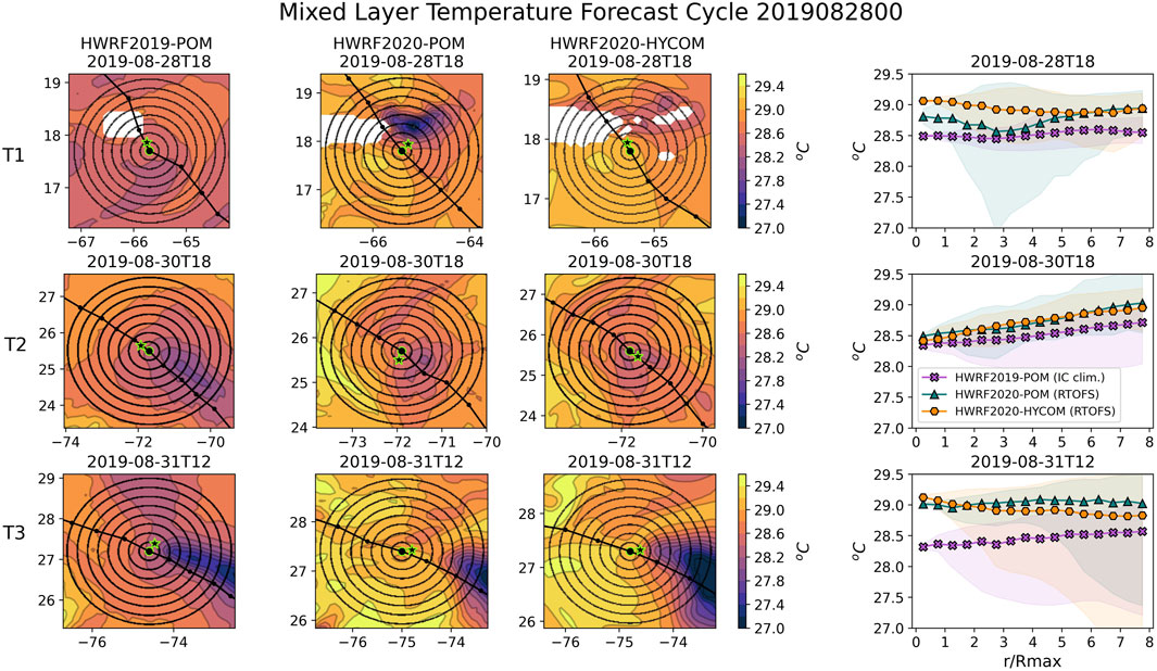
Figure 8. Mixed layer temperature (MLT) for three different forecast lead times for cycle 2019082800: 18 h (T1), 66 h (T2), and 84 h (T3) (shown in Figure 5) and for three hurricane forecasted models: HWRF2019-POM (IC Clim.), HWRF2020-POM (IC RTOFS), and HWRF2020-HYCOM (IC RTOFS). The circles are centered at the storm eye and show from 1 radius to 8 radius of maximum winds. The green start shows the location of the maximum winds. The last column shows the mean (markers) and the spread around the mean (shades) as a function of the normalized radius r/Rmax. For the calculation of the mean, the MLT field was grouped in bins of 0.5 normalized radius.

The SSHL per unit area is largest at the radius of maximum winds (eye wall region) in all cases (Figure 9), however there are marked spatial differences among the models. For instance on T3, SSHL values larger than 0.7 kJ/cm² are concentrated to a radius less than 2Rmax in HWRF2019-POM, while these values extent up to 4Rmax in the other two models, showing that the largest energy input from the ocean is found in a larger area in HWRF2020-POM and HWRF2020-HYCOM. Consistently HWRF2020-HYCOM is the model with the highest mean SSHL values for radii less than 4Rmax and HWRF2019-POM is the model with the lowest values for all radii for the three different times (Figure 9 right column).

Figure 9

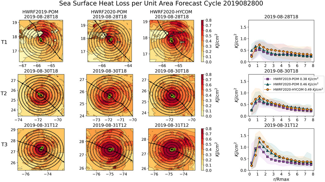
Figure 9. Sea surface heat loss (SSHL) per unit area for three different forecast lead times: 18 h (T1), 66 h (T2), and 84 h (T3) (shown in Figure 5) and for three hurricane forecasted models: HWRF2019-POM (IC Clim.), HWRF2020-POM (IC RTOFS), and HWRF2020-HYCOM (IC RTOFS). The circles are centered at the storm eye and show from 1 radius to 8 radius of maximum winds. The green start shows the location of the maximum winds. The last column shows the mean sea surface heat loss per unit area (markers) and the spread around the mean (shades) as a function of the normalized radius r/Rmax. For the calculation of the mean, the SSHL field was grouped in bins of 0.5 normalized radius. The figures correspond to the forecast cycle 2019082800.

Another quantity that reflects the differences in the spatial variability of SSHL is the area integrated SSHL, which provides information about the potential cumulative effect of an improved representation of air-sea fluxes along the hurricane track (Figure 10). This quantity is larger in HWRF2020-HYCOM for almost all lead times and as a consequence, the accumulated thermal energy input from the ocean to the atmosphere during the first 84 h is larger in HWRF2020-HYCOM by 17% compared to HWRF2019-POM. The same quantity is 12% higher in HWRF2020-POM than in HWRF2019-POM. Along with this result, we found that the MLT along the storm track for HWRF2019-POM is the coldest, about 0.5 degrees colder than HWRF2020-HYCOM (Figure 8, right column), for all forecast lead times. This implies that even a modest difference of about −0.5 degrees in the MLT can cause a cumulative decrease in the estimated total energy delivered from the ocean to the atmosphere of about 17% in a forecast cycle.

Figure 10

Figure 10. Area integrated sea surface heat loss as a function of forecast lead time. The area of integration is ± 2 degrees of longitude and latitude around the storm eye. The total energy delivered from the ocean to the atmosphere, which is the area under the curve, between 6 h and 84 h lead time for each model is shown in the legend of the figure.

4 Discussion and conclusion

Of the three coupled hurricane forecasting models evaluated, the model for which the ocean component was initialized from climatology, HWRF2019-POM, is the model with the largest MLT and OHC bias of −0.9°C and −18.8 kJ cm⁻², respectively, at the location and time of the glider observations during the passage of Hurricane Dorian North of Puerto Rico. In addition, this model is the hurricane forecasting model in which the ocean component has the lowest skill for the four metrics relevant to the air-sea heat fluxes assessed here.

Conversely, HWRF2020-HYCOM, initialized from RTOFS, is the hurricane forecasting model in which the ocean component has the highest skill for the four upper-ocean metrics and is the closest in skill to the data assimilative model GOFS 3.1. This gives us confidence that of the three air-sea coupled hurricane forecasting models evaluated, HWRF2020-HYCOM is the one that best represents the upper-ocean fields.

Nonetheless, HWRF2020-HYCOM and GOFS 3.1 do not excel in the upper-ocean metrics skills in spite of having a good skill to represent the temperature and salinity of the entire observed water column (down to 500 m). In particular, the salinity in the upper mixed layer was not properly represented. In this study, none of the models captured the salinity and depth of the barrier layer at the location of the glider array.

The barrier layer in the Caribbean Sea and tropical North Atlantic is caused by the spreading of the Amazon and Orinoco river plumes. The barrier layer spatial and vertical extend is controlled not only by the seasonal variability but also by the interannual variability of the river discharge (Hu et al., 2004), which cannot be captured by the ocean models studied here because only a monthly climatology river discharge was provided as input. This explains why salinity is rather ill-simulated and highlights the need to better take into account real-time river runoff, rather than monthly climatology, in ocean models, in addition to assimilate high quality in situ salinity.

Another aspect that needs improvement is the representation of vertical mixing processes in the surface boundary layer, which will lead to a better representation of the SST response during tropical cyclones. The traditional vertical mixing schemes, e.g., KPP mixing scheme, underpredict the vertical mixing in global models when compared to large eddy simulations. There exists vertical mixing parameterizations that include the effects of Langmuir turbulence that have shown to enhance vertical mixing when compared to the non-Langmuir schemes, but there are still large discrepancies on the estimate of the mixed layer depth among those (Li et al., 2019). Under hurricane wind conditions, there is evidence that including Langmuir turbulence can improve the SST evolution (Li et al., 2019; Zhou et al., 2023). In addition, Kim et al. (2022) demonstrates that the skill of 3-way coupled simulations for Hurricane Laura is improved over 2-way coupled forecasts, by explicitly including the Langmuir turbulence to the KPP mixing with HYCOM. This suggests that future hurricane forecast systems can improve the forecast skills by including a 3-way atmosphere-ocean-wave coupling.

Along hurricane Dorian’s forecasted track, the MLT in HWRF2019-POM is about −0.5 degrees colder than the MLT in HWRF2020-HYCOM. Accordingly, the area integrated and time integrated SSHL in HWRF2020-HYCOM is 17% higher than the SSHL in HWRF2019-POM during the first 84 h of the forecast cycle. This result indicates that even differences of several tenths of a degree in the MLT in hurricane forecasting models, can lead to substantial differences in the total enthalpy fluxes delivered from the ocean to the atmosphere throughout the storm’s synoptic history.

The upper-ocean fields assessed in this work, which are relevant to the air-sea heat fluxes, were not accurately represented in the three coupled atmosphere-ocean hurricane forecasting models evaluated here, and need to be better captured on future models currently under development. In particular, a more accurate representation of barrier layers could improve the model forecast skill during storms. This work also shows that large biases in the upper-ocean conditions can be introduced if the ocean model is initialized with climatological temperature and salinity fields. Therefore, there is a critical need to improve the upper-ocean initial conditions leading to better ocean representation in coupled atmosphere-ocean models, as part of the larger effort to improve the different aspects that control the hurricane intensity forecast.

In addition, this study demonstrates a methodology to assess a model skill of the upper-ocean conditions that contribute to the TC intensity forecast, and it makes the case that the upper-ocean profile observations of temperature and salinity are a very valuable asset to help improve, through data assimilation techniques, the ocean representation, particularly of barrier layers and of ocean heat content, which have been linked to hurricane intensity changes.

Data availability statement

The original contributions presented in the study are included in the article. Further inquiries can be directed to the corresponding author.

Author contributions

MA: Conceptualization, Formal Analysis, Software, Visualization, Writing–original draft. H-SK: Conceptualization, Resources, Writing–review and editing. ML: Conceptualization, Funding acquisition, Writing–review and editing. TM: Conceptualization, Funding acquisition, Writing–review and editing. SG: Conceptualization, Funding acquisition, Writing–review and editing. GG: Conceptualization, Funding acquisition, Writing–review and editing.

Funding

The authors declare that financial support was received for the research, authorship, and/or publication of this article. The author MA was supported by the NOAA Integrated Ocean Observing System (IOOS) through the award NA16NOS0120020. This work was also supported by the Disaster Related Appropriation Supplemental: Improving Forecasting and Assimilation (DRAS 19 IFAA), award NA19OAR0220184, and NA19OAR0220189. It was also supported by the FY19 Disaster Supplemental: Improving Forecasting of Hurricanes, Floods, and Wildfires (FY 19 IFHFW) award NA20OAR4600263. ML was partly supported under the auspices of the Cooperative Institute for Marine and Atmospheric Studies (CIMAS), a cooperative institute of the University of Miami and NOAA, cooperative agreement NA20OAR4320472. GG and ML were supported by NOAA/AOML. TM and SG were supported by Rutgers University.

Acknowledgments

This work was a collaboration between NOAA NOS, NWS and OAR researchers. We thank Ben LaCour for his help to get access to the NOAA high performance computing platforms. We also thank all the sponsors, institutions and researchers that provided their glider data to the IOOS Glider DAC.

Conflict of interest

Author MA was employed by Lynker at NOAA/NCEP/EMC.

The remaining authors declare that the research was conducted in the absence of any commercial or financial relationships that could be construed as a potential conflict of interest.

The authors declared that they were an editorial board member of Frontiers, at the time of submission. This had no impact on the peer review process and the final decision.

Publisher’s note

All claims expressed in this article are solely those of the authors and do not necessarily represent those of their affiliated organizations, or those of the publisher, the editors and the reviewers. Any product that may be evaluated in this article, or claim that may be made by its manufacturer, is not guaranteed or endorsed by the publisher.

References

Avila, L., Stewart, S., Berg, R., and Ab, H. (2020). Tropical cyclone report hurricane Dorian (al052019). Miami, FL, USA: National Hurricane Center. 24 August–7 September 2019.

Google Scholar

Balaguru, K., Chang, P., Saravanan, R., Leung, L. R., Xu, Z., Li, M., et al. (2012). Ocean barrier layers’ effect on tropical cyclone intensification. Proc. Natl. Acad. Sci. 109 (36), 14343–14347. doi:10.1073/pnas.1201364109

PubMed Abstract | CrossRef Full Text | Google Scholar

Balaguru, K., Foltz, G. R., Leung, L. R., Kaplan, J., Xu, W., Reul, N., et al. (2020). Pronounced impact of salinity on rapidly intensifying tropical cyclones. Bull. Am. Meteorological Soc. 101 (9), E1497–E1511. doi:10.1175/bams-d-19-0303.1

CrossRef Full Text | Google Scholar

Biswas, M. K., Abarca, S., Bernardet, L., Ginis, I., Grell, E., Iacono, M., et al. (2018). Hurricane weather research and forecasting (hwrf) model: 2018 scientific documentation. https://dtcenter.org/HurrWRF/users/docs/scientificdocuments/HWRFv4.0aScientificDoc.pdf.

Google Scholar

Carnes, M. J. (2009). Description and evaluation of GDEM-V 3.0. Washington, DC, USA: Naval Research Laboratory technical report, 27. NRL/MR/7330--09-9165.

Google Scholar

Chen, S. S., Price, J. F., Zhao, W., Donelan, M. A., and Walsh, E. J. (2007). The CBLAST-Hurricane program and the next-generation fully coupled atmosphere–wave–ocean models for hurricane research and prediction. Bull. Am. Meteorological Soc. 88 (3), 311–318. doi:10.1175/bams-88-3-311

CrossRef Full Text | Google Scholar

Cione, J. J., and Uhlhorn, E. W. (2003). Sea surface temperature variability in hurri-canes: implications with respect to intensity change. Mon. Weather Rev. 131 (8), 1783–1796. doi:10.1175//2562.1

CrossRef Full Text | Google Scholar

Cummings, J. A., and Smedstad, O. M. (2013). “Variational data assimilation for the Global Ocean,” in Data assimilation for atmospheric, oceanic and hydrologic applications. Editors S. Park, and L. Xu (Berlin, Germany: Springer), II, 303–343. Chapter 13.

CrossRef Full Text | Google Scholar

de Boyer Montégut, C., Madec, G., Fischer, A. S., Lazar, A., and Iudicone, D. (2004). Mixed layer depth over the global ocean: an examination of profile data and a profile-based climatology. J. Geophys. Res. Oceans 109 (C12). doi:10.1029/2004jc002378

CrossRef Full Text | Google Scholar

de Ruijter, W. P. (1983). Effects of velocity shear in advective mixed-layer models. J. Phys. Oceanogr. 13 (9), 1589–1599. doi:10.1175/1520-0485(1983)013<1589:eovsia>2.0.co;2

CrossRef Full Text | Google Scholar

Domingues, R., Goni, G., Bringas, F., Lee, S. K., Kim, H. S., Halliwell, G., et al. (2015). Upper-ocean response to Hurricane Gonzalo (2014): salinity effects revealed by targeted and sustained underwater glider observations. Geophys. Res. Lett. 42 (17), 7131–7138. doi:10.1002/2015gl065378

CrossRef Full Text | Google Scholar

Domingues, R., Kuwano-Yoshida, A., Chardon-Maldonado, P., Todd, R. E., George, H., Kim, H.-S., et al. (2019). Ocean observations in support of studies and forecasts of tropical and extratropical cyclones. Front. Mar. Sci. 6, 446. doi:10.3389/fmars.2019.00446

CrossRef Full Text | Google Scholar

Dong, J., Domingues, R., Goni, G., George, H., Kim, H.-S., Lee, S.-K., et al. (2017). Impact of assimilating underwater glider data on Hurricane Gonzalo (2014) forecasts. Weather Forecast. 32 (3), 1143–1159. doi:10.1175/waf-d-16-0182.1

CrossRef Full Text | Google Scholar

Emanuel, K. A. (1986). An air-sea interaction theory for tropical cyclones. part i: steady-state maintenance. J. Atmos. Sci. 43 (6), 585–605. doi:10.1175/1520-0469(1986)043<0585:aasitf>2.0.co;2

CrossRef Full Text | Google Scholar

Emanuel, K. A. (1999). Thermodynamic control of hurricane intensity. Nature 401 (6754), 665–669. doi:10.1038/44326

CrossRef Full Text | Google Scholar

Garraffo, Z. D., Cummings, J. A., Paturi, S., Hao, Y., Iredell, D., Spindler, T., et al. (2020). “RTOFS-DA: real Time Ocean-Sea Ice coupled three dimensional variational global data assimilative ocean forecast system,” in Research activities in Earth system modelling. Editor E. Astakhova (Geneva, Switzerland: WMO, World Climate Research Program Report No.6) July, 2020).

Google Scholar

GDAS/GFS v15.0.0 (2018). Implementation of NGGPS/FV3GFS V1.0, GDAS/GFS V15.0.0 for Q2FY2019. https://www.emc.ncep.noaa.gov/emc/docs/FV3GFS_OD_Briefs_10-01-18_4-1-2019.pdf.

Google Scholar

Glenn, S., Miles, T., Seroka, G., Xu, Y., Forney, R., Yu, F., et al. (2016). Stratified coastal ocean interactions with tropical cyclones. Nat. Commun. 7 (1), 10887–10910. doi:10.1038/ncomms10887

PubMed Abstract | CrossRef Full Text | Google Scholar

Halliwell, G., Shay, L. K., Brewster, J., and Teague, W. J. (2011). Evaluation and sensitivity analysis of an ocean model response to hurricane ivan. Mon. Weather Rev. 139 (3), 921–945. doi:10.1175/2010mwr3104.1

CrossRef Full Text | Google Scholar

Hu, C., Montgomery, E. T., Schmitt, R. W., and Muller-Karger, F. E. (2004). The dispersal of the amazon and orinoco river water in the tropical atlantic and caribbean sea: observation from space and s-palace floats. Deep Sea Res. Part II Top. Stud. Oceanogr. 51 (10-11), 1151–1171. doi:10.1016/j.dsr2.2004.04.001

CrossRef Full Text | Google Scholar

Jaimes, B., Shay, L. K., and Halliwell, G. R. (2011). The response of quasigeostrophic oceanic vortices to tropical cyclone forcing. J. Phys. Oceanogr. 41 (10), 1965–1985. doi:10.1175/jpo-d-11-06.1

CrossRef Full Text | Google Scholar

Jaimes, B., Shay, L. K., and Uhlhorn, E. W. (2015). Enthalpy and momentum fluxes during hurricane earl relative to underlying ocean features. Mon. Weather Rev. 143 (1), 111–131. doi:10.1175/mwr-d-13-00277.1

CrossRef Full Text | Google Scholar

Kim, H.-S., Lozano, C., Tallapragada, V., Iredell, D., Sheinin, D., Tolman, H. L., et al. (2014). Performance of ocean simulations in the coupled hwrf–hycom model. J. Atmos. Ocean. Technol. 31 (2), 545–559. doi:10.1175/jtech-d-13-00013.1

CrossRef Full Text | Google Scholar

Kim, H. S., Meixner, J., ThomasReichl, B. G. B., Liu, B., Mehra, A., Wallcraft, A., et al. (2022). Skill assessment of NCEP three-way coupled HWRF–HYCOM–WW3 modeling system: hurricane Laura case study. Weather Forecast. 37 (8), 1309–1331. doi:10.1175/waf-d-21-0191.1

CrossRef Full Text | Google Scholar

Large, W. G., McWilliams, J. C., and Doney, S. C. (1994). Oceanic vertical mixing: a review and a model with a nonlocal boundary layer parameterization. Rev. Geophys. 32 (4), 363–403. doi:10.1029/94rg01872

CrossRef Full Text | Google Scholar

Le Hénaff, M., Domingues, R., Halliwell, G., Zhang, J. A., Kim, H.-S., Aristizabal, M., et al. (2021). The role of the Gulf of Mexico ocean conditions in the intensification of Hurricane Michael (2018). J. Geophys. Research–Oceans 126 (5), e2020JC016969. doi:10.1029/2020jc016969

CrossRef Full Text | Google Scholar

Leipper, D. F., and Volgenau, D. (1972). Hurricane heat potential of the Gulf of Mexico. J. Phys. Oceanogr. 2 (3), 218–224. doi:10.1175/1520-0485(1972)002<0218:hhpotg>2.0.co;2

CrossRef Full Text | Google Scholar

Li, Q., Reichl, B. G., Fox-Kemper, B., Adcroft, A. J., Belcher, S. E., Danabasoglu, G., et al. (2019). Comparing ocean surface boundary vertical mixing schemes including Langmuir turbulence. J. Adv. Model. Earth Syst. 11 (11), 3545–3592. doi:10.1029/2019ms001810

CrossRef Full Text | Google Scholar

Mainelli, M., DeMaria, M., Shay, L. K., and Goni, G. (2008). Application of oceanic heat content estimation to operational forecasting of recent atlantic category 5 hurricanes. Weather Forecast. 23 (1), 3–16. doi:10.1175/2007waf2006111.1

CrossRef Full Text | Google Scholar

Malkus, J. S., and Riehl, H. (1960). On the dynamics and energy transformations in steady-state hurricanes. Tellus 12 (1), 1–20. doi:10.3402/tellusa.v12i1.9351

CrossRef Full Text | Google Scholar

Metzger, E. J., Helber, R. W., Hogan, P. J., Posey, P. G., Thoppil, P. G., Townsend, T. L., et al. (2017). Global ocean forecasting system 3.1, validation test. Washington, DC, USA: Naval Research Laboratory. NRL/MR/7320—17-9722.

Google Scholar

Miles, T., Seroka, G., and Glenn, S. (2017). Coastal ocean circulation during hurricane sandy. J. Geophys. Res. Oceans 122 (9), 7095–7114. doi:10.1002/2017jc013031

CrossRef Full Text | Google Scholar

Miles, T. N., Zhang, D., Foltz, G. R., Zhang, J. A., Meinig, C., Bringas, F., et al. (2021). Uncrewed ocean gliders and saildrones support hurricane forecasting and research. Oceanography 34 (4), 78–81. doi:10.5670/oceanog.2021.supplement.02-28

CrossRef Full Text | Google Scholar

Price, J. (2009). Metrics of hurricane-ocean interaction: vertically-integrated or vertically-averaged ocean temperature? Ocean Sci. 5 (3), 351–368. doi:10.5194/os-5-351-2009

CrossRef Full Text | Google Scholar

Rhodes, R. C., Hurlburt, H. E., Wallcraft, A. J., Barron, C. N., Martin, P. J., Metzger, E. J., et al. (2001). Navy real-time global modeling systems. Washington, DC, USA: NAVAL RESEARCH LAB STENNIS SPACE CENTER MS OCEANOGRAPHY DIV.

Google Scholar

Rudzin, J. E., Shay, L. K., and Benjamin Jaimes de la, C. (2019). The impact of the Amazon–Orinoco River plume on enthalpy flux and air–sea interaction within Caribbean Sea tropical cyclones. Mon. weather Rev. 147 (3), 931–950. doi:10.1175/mwr-d-18-0295.1

CrossRef Full Text | Google Scholar

Shay, L. K., and Eric, W. U. (2008). Loop current response to hurricanes isidore and lili. Mon. weather Rev. 136 (9), 3248–3274. doi:10.1175/2007mwr2169.1

CrossRef Full Text | Google Scholar

Shay, L. K., Goni, G. J., and Black, P. G. (2000). Effects of a warm oceanic feature on hurricane opal. Mon. Weather Rev. 128 (5), 1366–1383. doi:10.1175/1520-0493(2000)128<1366:eoawof>2.0.co;2

CrossRef Full Text | Google Scholar

Taylor, K. E. (2001). Summarizing multiple aspects of model performance in a single diagram. J. Geophys. Res. Atmos. 106 (D7), 7183–7192. doi:10.1029/2000jd900719

CrossRef Full Text | Google Scholar

Whitaker, W. D. (1967). Quantitative determination of heat transfer from sea to air during passage of hurricane betsy. Unpublished doctoral dissertation. College Station, TX, USA: Texas A&M University.

CrossRef Full Text | Google Scholar

Zhang, J. A., Black, P. G., French, J. R., and Drennan, W. M. (2008). First direct measurements of enthalpy flux in the hurricane boundary layer: the CBLAST results. Geophys. Res. Lett. 35 (14). doi:10.1029/2008gl034374

CrossRef Full Text | Google Scholar

Zhou, X., Hara, T., Ginis, I., D’Asaro, E., and Reichl, B. G. (2023). Evidence of Langmuir mixing effects in the upper ocean layer during tropical cyclones using observations and a coupled wave-Ocean Model. J. Geophys. Res. Oceans 128 (10), e2023JC020062. doi:10.1029/2023jc020062

CrossRef Full Text | Google Scholar