(DA-DOPF): A Day-Ahead Dynamic Optimal Power Flow With Renewable Energy Integration in Smart Grids

1 Introduction

Optimal power flow (OPF) is an efficient and legitimately organized tool to control the settings of decision variables of the power system. The trade-off can be accomplished between the economy and the security of the power system by getting an ideal arrangement of these control factors. In this manner, OPF is a critical tool to give an ideal arrangement of control boundaries while fulfilling the imperatives (Surender Reddy et al., 2014; Surender Reddy et al., 2017). Generally, the OPF problem is formulated as a highly complex and non-linear optimization problem due to finding the feasible values in a large number of continuous and discrete control variables (Carpentier, 1962). Moreover, equality and inequality constraints can further enhance its computational complexity. OPF can also be integrated with other energy management systems (EMSs), to provide preventive and secure modes of operation. In the preventive mode, they can prevent frequency-mode problems which can be worse in terms of the blackout, while in the secure mode, they made corrective changes in the power flow pattern to provide feasible economic conditions. Researchers have been involved in the development of OPF to make it more reliable and to get optimal solutions with fast convergence (Momoh et al., 1997).

Since the OPF study provides the knowledge of feasible control variables under constraints on different variables, they are a major tool for the reliable operation of the power system. The significance of OPF issue is very much distinguished, and different old-style strategies, for example, gradient method (GM) (Dommel and Tinney, 1968a; Lee et al., 1985), Newton algorithm (NA) (Talukdar et al., 1983; Sun et al., 1984), linear programming (LP) (Fahd and Sheble, 1992), and quadratic programming (QP) (Reid and Hasdorff, 1973) have been applied to tackle the issues of being trapped in local minima, step size, and slow convergence. Recently, hybrid energy systems are getting more importance in which energy sources of two or more forms are combined. This combination minimizes the different attributes of the power system such as cost, loss, and emission and also increases the reliability and the life span of the power system (Chedid and Rahman, 1997; Chedid et al., 2000). Hence, hybrid renewable energy systems (HRESs) are becoming popular these days, even though the intermittency of VESs is a problem to integrate these sources. However, the combination of different renewable energy sources compensates each other to improve the stochastic nature of these sources (Banos et al., 2011; Ahn et al., 2012). There are two types of HRESs, standalone and grid-connected. Standalone systems have storage devices to fulfill load demands in a time of shortage of solar or wind energy. Though on account of the framework-associated system, storage devices can be taken out as the power deficiency can be repaid from the network power. These network-associated HRESs give power either to the heap or to the matrix, where in grid-connected systems, the power electronics converters are installed to address the issues of frequency, voltage stability, reactive power compensation, harmonics filtering, and load sharing. HRESs can be further classified into two categories: island HRESs and grid-connected HRESs. Island HRESs supply to the local loads, while grid-connected HRESs are those in which RESs are at distributed places.

The generation cost minimization is one of the common objectives of OPF by finding the optimal combination of generators, and this can be considered an economic dispatch problem. Due to pollution issues, this economic dispatch (ED) problem can be further solved as an economic environmental dispatch (EED) problem. Furthermore, depleting reserves of fossil fuel and global warming issues forced the energy-based research toward the utilization of clean and green energy sources. Nevertheless, uncertainties of these weather-driven renewable energy sources make it difficult to schedule dispatchable generation. With the increase in the penetration of clean and green electricity generation sources like wind and solar (PV), it is necessary to guide research toward the formulation of generation scheduling problem by paying attention to the intermittent and non-dispatchable characteristics of such sources. Since wind and solar are free and abundant in nature, penetration of these VESs minimizes the overall cost of electricity generation. Moreover, the voltage stability of the power system is always at stake due to the increasing electricity demand. Therefore, OPF algorithms are quite capable of handling the voltage stability issue by managing the power flow in transmission lines.

While paying attention to the scheduling of non-dispatchable sources of energy, it is desirable to incorporate artificial intelligence (AI) and machine learning (ML) algorithms with the traditional OPF program. Nowadays, AI and ML algorithms are performing tasks much like a human would do. In particular, artificial neural networks (ANNs) can predict process models for process control using the data collected by the sensors and transducers. Moreover, these algorithms are capable of learning patterns and producing results in alternate ways instead of doing hectic calculations. They are inspired by the biological neural system of the human brain and are capable of duplicating the learning, consolidation, adaptation, and generalization skills of the human brain (McCulloch and Walter, 1943). When it comes to non-linear problems, ANNs are the most powerful tools to solve them. ANNs consist of neurons, which are the highly interconnected processing units. Information is passed between these neurons. Each neuron decides based on two input values: one is an input and the other is the weight. The ANNs are not developed to perform a specific task; in fact, they are designed to learn patterns by gathering, storing, and generalizing information. ANNs consist of many layers, and to reach the target, different stochastic algorithms renew the weights of ANNs. The backpropagation network (BPN) is the most common algorithm to update weights in the ANN (İnal and Aras, 2005). In the past decade, the use of ANNs has been increasing substantially, and this is due to their versatility, robustness, availability of data, and increased computational power. Their ability to learn from sequence patterns enables ANNs to work with noise data, fuzzy information, and non-linear and ill-defined problems. Their fault tolerance capability further expands the implementation of ANNs. Recently, ANNs have become an ideal tool to apply in the fields of medicine, economics, meteorology, psychology, neurology, and many others. Medical imaging, identification of military targets, market forecasting, weather forecasting, flood forecasting, and electrical and thermal load forecasting are some common examples of ANN applications.

It is suggested that the integration of VESs enhances the overall efficiency of the existing grid. However, it is an obvious fact that these sources are weather dependent like a photovoltaic (PV) cell depending on solar irradiance or sunlight intensity to produce electrical energy. Similarly, wind turbines produce electrical energy by using the natural pressure of the wind. Moreover, this natural dependence forces the utility to install these generation sources at distributed places, which are favorable for these sources in regard to electricity generation. Although these VESs bring stability and reliability to the power system and are the cause of a green and clean environment, yet many concerns are associated with the integration of these VESs into the existing grid. The intermittent nature of these VESs makes it difficult to guess the available power from these sources. However, the utility needs to know the available power to estimate the reserve capacity of the generation system. Additionally, on the facade of force framework activity and control, the circulated idea of these sources and a variety of inaccessible forces makes it hard to set the estimations of control factors of the force framework. Subsequently, the force framework administrator needs notable anticipated estimations of these control factors to keep up the overall influence stream in the framework. Along these lines, there is space to build up a strategy to give the most plausible estimations of control factors of the force framework to the framework administrator. In such a manner, the proposed strategy will utilize an ANN model to anticipate the breeze and sunlight–based irradiance for wind and sun–oriented age plants. Afterward, it will foresee the practical warm age plants to limit the age cost regarding punishment cost, save cost, and all-out cost. In doing so, we need to make sure that the variables of the power system will remain within their boundary limits. Therefore, the power system will remain at its state of equilibrium.

From the above discussion, it is revealed that there is enough room to propose the optimal scheduling strategy, which can handle the intermittency of VESs. This study is presented to solve the power flow problem in a dynamic power system. The major components of this dynamic power system are conventional thermal generators, wind farms, and solar PV plants. The key problem of this study is to schedule these power generation sources at optimal values. Moreover, along with different constraints of the power system, the problem becomes more complicated. Furthermore, VESs like wind and solar generators cannot be scheduled in the same manner as conventional thermal generators, due to the inherent property of weather dependency, e.g., wind velocity and solar irradiation. The uncertainty and intermittency of these VESs make this challenge more difficult. In addition to this, load on a power system is variable, and the availability of VESs is irrelevant to this variable load. A system operator cannot know the actual real-time (RT) conditions for a specified day-ahead (DA) schedule. To solve this day-ahead dynamic optimal power flow (DA-DOPF) problem, an RT-OPF problem is integrated with the ANN model to predict the wind speed and solar irradiance. Therefore, the novelty of the proposed DA-DOPF approach is a two-stage optimization approach consisting of an LM algorithm–based ANN model and particle swarm optimization–based economic load dispatch along with OPF problem constraints with an effective constraint handling technique. The former precisely generates the available power of VESs with respect to the wind speed and solar irradiance, and the latter provides the best-fit generation schedule of the generation sources along with the satisfaction of power system constraints. Our proposed study characterizes the structure of the predicted output of the ANN model and RT-OPF. And to the best of authors’ knowledge, it is not presented in the previous existing literature. Furthermore, the main contribution of the present study is listed in the next section.

1.1 Contribution of the Paper

The real contributions of this work are given as follows:

• The improvement in RT-OPF is evaluated by incorporating ANN-based predictive modeling in the OPF program. Here, the ANN uses real and noticed climatic information which incorporates both meteorological changes and barometric impacts, such as temperature and overcast cover.

• Improvement in loss minimization is achieved by using the Levenberg–Marquardt (LM) algorithm for the adopted three-layer shallow ANN (Section VI).

• An efficient constraint handling technique is adopted to guide the search process toward a global optimal solution and thoroughly discussed in Section IV-E.

• Real-time scheduling of generation sources is achieved in a single run of the program by incorporating T-FMF, to compute the CFs at the start of DA-DOPF.

• A systematic approach is used to combine all the above-mentioned techniques with a particle swarm optimization (PSO) economic dispatched algorithm for the IEEE 30-bus system, and critical analysis of simulation results has been done to identify the effectiveness of the proposed approach.

Simulations results depict that the proposed approach efficiently handles the complexities of the OPF problem. Moreover, the present study shows the efficient integration of RESs and maximum power utilization from these sources can be made possible by using NNs.

The remainder of this paper is organized as follows: Section II presents literature review. Section III provides details of inspiration. Section IV presents the numerical demonstration and issue definition. Section V gives the force models of VESs. The breeze and sun–oriented determining models are discussed in Section VI. The proposed DA-DOPF approach is introduced in Section VII. The results and conversations are examined in detail in Section VIII. Conclusions are outlined in Section IX.

2 Literature Review

As of late, the OPF issue has acquired a lot of consideration from scientists since OPF is an essential requirement for the smooth and dependable activity of the power system. The power system administrator needs to limit the general age cost, limit system misfortune, and keep up as far as possible by controlling the responsive power stream in the current transmission system. Subsequently, OPF is a fundamental instrument for power system administrators in the activity and control of power systems. Notwithstanding, because of the non-linear and non-convex nature alongside different limitations, numerous calculations and improvement methods are created to tackle the OPF issue. These methods are comprehensively grouped into two classifications: 1) traditional advancement procedures and 2) transformative enhancement strategies. A wide assortment of traditional improvement strategies have been utilized to tackle OPF such as non-straight programming (Dommel and Tinney, 1968b; Alsac and Stott., 1974; Happ, 1977; Mamandur and Chenoweth, 1981; Shoults and Sun, 1982; Habibollahzadeh et al., 1989), direct programming (Stadlin and Fletcher, 1982; Mota-Palomino and Quintana, 1986; Abou El-Ela and Abido, 1992), quadratic programming (Reid and Lawrence, 1973; Burchett et al., 1984; Aoki et al., 1987), Newton-based procedures (Sun et al., 1984; Santos and Da Costa, 1995), successive unconstrained minimization strategy (Rahli and Pirotte, 1999), and inside-point techniques (Momoh and Zhu, 1999). All these techniques for streamlining have some normal disadvantages such as issues of non-assembly, non-direct target capacities and requirements, introductory supposition, and step size. A nitty gritty overview identified with these issues is introduced by Momoh et al. (1999a) and Momoh et al. (1999b). For the most part, these old-style methods use inclination-based advancement calculations to linearize the goal work. The OPF issue is profoundly non-direct and has numerous neighborhood minima, for example, multi-modal, so these procedures do not perform well to track down the doable arrangement. Moreover, the OPF issue is non-differentiable, non-smooth, and non-curved, while these procedures depend on inclination strategies. In this manner, it is fundamental to grow such methods that can beat these challenges. As of late, on the facade of transformative calculations, new improvement procedures have been created. These high-level enhancement procedures are computationally effective, quick, and solid. These techniques do not suffer from convergence issues and local optimality. Some common examples of these techniques are genetic algorithm (GA) (Lai et al., 1997), Osman et al.’s algorithm (Osman et al., 2004), simulated annealing (SA) by Miranda et al. (1998), tabu search (TS), and PSO (Abido, 2002a; Abido, 2002b), respectively. With due respect to these advanced techniques, unfortunately, it has been found that they have a problem of pre-mature convergence and parameter selection. It is difficult to fine-tune the parameters of these algorithms and to handle constraints. These difficulties lead to the infeasible solution, computational time complexities. Therefore, there is always a trade-off between the complexity and the solution.

In AlRashidi and El-Hawary (2009) and Frank et al. (2012), the detailed comparison to solve the OPF problem is discussed. Improved GA has been used to find the feasible values of control variables of the load flow problem by Lai et al. (1997). In Abido et al. (2002b), the PSO algorithm is used while solving an OPF problem. Variants of PSO are presented by Kennedy and Russell (1995), Kennedy (2000), Saber et al. (2007), Dutta and Singh (2008), and Gnanadass and Venkataramana (2008). Niknam et al. (2012a) examined an improved PSO to streamline the various goals of OPF at the same time while considering generator fuel cost, genuine power misfortune, fossil fuel byproduct, and solidness file of voltage as numerous targets for enhancement. In the work of Niknam et al. (2012b), the shuffle frog leaping algorithm (SFLA) and SA have acquainted with managing the non-bended nature of old enough expense target work. The ideal estimations of control factors have been accomplished utilizing a versatile genuine coded biogeography–based improvement calculation; subsequently, precision and heartiness are observers in the aftereffects of OPF (Ramesh Kumar and Premalatha, 2015). The ideal power stream issue is introduced as a multi-target enhancement issue and has been settled utilizing a concordance search calculation with an all-encompassing quick non-ruled arranging and positioning method, so the best trade-off arrangement is extricated in various cases (Sivasubramani and Swarup, 2011). Recently, the conventional stochastic methods were also used for weather prediction. Muneer and Gul (2000) and Muneer et al. (2000) presented another forecasting model based on meteorological radiations and cloud cover radiations for solar radiations. All these mathematical stochastic models and probability density functions use radiation theories and meteorological data collected by sensors to predict the solar radiations (Tobiska, 2000; Reddy and Ranjan., 2003). Additionally, for wind speed anticipating, analysts have built up certain models, because of recursive least-squares relapse or auto-regressive coordinated moving normal techniques, much precisely figure on account of noticed time-arrangement information and their connections (Giebel et al., 2003; Landberg et al., 2003).

Similarly, after the development of the probabilistic optimal power flow (POPF), the direction of research is shifted toward the development of model and calculation methods. In Huynh et al. (2018), the probabilistic power flow methodology for large-scale power systems incorporating renewable energy sources is presented. Dynamic radial basis functions of neural networks are used to generalize three-phase robust load flow for radial and meshed power systems with and without uncertainty in energy resources (Baghaee et al., 2018). The Markov chain quasi-Monte-Carlo sampling method is utilized to perform POPF with correlated wind power uncertainty in Sun et al. (2019). In Wang and Guo (2018), a real-time power balancing critical time scale is achieved with intermittent power sources. The bidding methodology in a joint hydro-electric and wind park is proposed by Kneevi et al. (2019). Baghaee et al. (2017) introduced the fuzzy unscented transform for uncertainty quantification of correlated wind/PV microgrids. An efficient approach for practical approximations and heuristic approaches for managing shiftable loads in the multi-period optimal power flow are discussed by Avramidis et al. (Iason-Iraklis et al., 2021).

As of late, ANNs are the focal point of consideration for sun and wind–oriented gauging because of their characteristic ability to deal with the non-linearities of forecast goals (Kalogirou, 2000). Furthermore, integration of fuzzy rules and wavelet transformation with NNs gives new directions to the research by Barbounis et al. (2006), Cao and Cao (2006), and Chaabene and Ben Ammar (2008). Moreover, to reduce the prediction error and to enhance the convergence rate, different algorithms are presented by the researchers in recent literature. Mishra et al. (2015) published a scaled conjugate algorithm to train an MLP-based ANN for least squares (LS) and minimum mean square error (MMSE). Stefenon et al. (2020) presented the well-known BFGS quasi-Newton optimization method to achieve better performance of the ANN. Plumb et al. (2005) discussed the predictive ability of artificial neural network (ANN) models along with four classes of training algorithms.

It has been found in the previous literature that constraint handling techniques are not considered in a day-ahead OPF problem along with the prediction of available real power from VESs. Moreover, the complexity of real-time OPF is pretty much high due to the multiple runs of the program. The idea presented in this work is different from that of the earlier proposed work, and its focus is on the prediction of solar irradiance and wind speed by the ANN, and then it is used to calculate the available power from these VESs. In addition to this, the LM algorithm is used to minimize the prediction error and to increase the convergence rate of the ANN. Along with this, T-FMF is used to calculate the CFs for VESs in each sub-interval. The SF solution constraint handling approach is used to handle constraint violation. Moreover, 24-h variable load is assumed to be known, and each 1-h interval is subdivided into six sub-intervals each of 10 min to find the values of control variables to convert the conventional OPF into the DA-DOPF. In the end, the optimal schedule of generation sources and feasible values of control variables are presented in Section VIII for each sub-interval, which shows the effectiveness of the study.

3 Problem Overview and Motivation

This work considers and solves the OPF problem of the power system having multiple VESs. The main components of this system comprise the conventional thermal generators, wind farms, and solar PV plants on different buses. The scheduling of generation sources in such a system is a challenging task due to the integration of VESs because VESs are weather dependent and a little change in climate conditions may affect the available output power of these sources. Moreover, the load is variable, and the power system operator is responsible to fulfill this load demand by scheduling the generation sources at the optimal generation point. In a hybrid system, an optimal scheduling approach is presented by Yang et al. (2013) to manage a wind, solar, and storage system. Gayme and Topcu (2012) figured an OPF issue to track down the ideal estimations of factors of a power system having a capacity limit. Levron et al. (2013) introduced a strategy to deal with the capacity gadgets of the microgrid. The customary OPF is a static improvement issue in a power system having no wellspring of shifting yield power like solar and wind. In conventional OPF, the lone goal is to satisfy the heap need by running the OPF program at various stretches. To take care of the OPF issue with the wind age, the creators utilized the stochastic model to anticipate the wind speed by Jabr et al. (Jabr and Pal, 2009). Here, the OPF issue is defined to limit the fossil fuel byproduct, power misfortune, and age cost with and without valve point impact in Dubey et al. (2015). The issue with infiltration of wind age and DC OPF is tackled by Zhang and Giannakis (2013). Nowadays, the integration of renewable energy is rapidly expanding and trending in many power systems of the world. VESs are principally nature-friendly and contamination-free, and they can serve longer as compared to conventional generation sources. However, VESs are weather dependent, and therefore, available real power is always variable. For example, cloud cover on a clear day suddenly decreases an available output power from the PV plant. Similarly, variation in wind speed affects the available output power of wind turbines. Therefore, power output from these sources varies from minute to minute scale. Hence, the power system operator needs an efficient power flow program that is capable of running again and again to maintain power flow in the system by scheduling generation sources, managing tap changing, and connecting and disconnecting VAR compensation devices. Although the methods reported earlier are quite capable of solving the OPF problem, there is an opportunity available to develop a new technique to solve OPF dynamically. Hence, the motivation behind this study is listed as follows:

• ANNs are incorporated to schedule the generation sources more accurately.

• An efficient constraint handling approach is considered to find the most feasible solution.

• To reduce the complexity of the OPF program, contribution factors (CFs) are calculated prior to running the load flow for each sub-interval.

Therefore, in this study, the ANN is used to predict the meteorological values for the power models of solar and wind power generators, and CFs are calculated using T-FMF, before going into the load flow loop of the program. Furthermore, to guide the search process of optimization toward a feasible solution, the SF constraint handling technique is used in the single run of the DA-DOPF program. And to the best of the authors’ knowledge, such a mechanism has not been developed before to solve the real-time OPF.

4 DA-DOPF Problem Formulation

The DA-DOPF problem is formulated as an optimization problem with the objective of minimizing generation cost of conventional thermal generators along with the cost equations of VESs. A general optimization problem subjected to constraints can be expressed as follows: minimize:

$min\{f(a,b)=f1(a,b)\}(1)$

subject to

$g_j(a,b)\ge 0,j=\mathrm{1,2},\dots ,M,(2)$

$h_k(a,b)=0,k=\mathrm{1,2},\dots ,N,(3)$

where $a={\{a^1,a^2,\dots ,a^n\}}^T$ represents a vector of independent decision variables and $b={\{b^1,b^2,\dots ,b^n\}}^T$ represents the dependent decision variable vector. The inequality constraints are g_j (a, b) where j = {1, 2, …, M, }, and the equality constraints are h_k (a, b), where k = {1, 2, …, N}. Total numbers of inequality and equality constraints are M and N, respectively. Table 1 shows the state and control variables.

TABLE 1

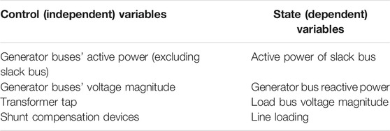
TABLE 1. Control and dependent variables.

Def. 1. Control (independent) variables: The following equation represents a set of control variables:

$b=\{(P_{G2},‥,P_{GN}),(V_{G1},‥,V_{GN}),(Q_{C1},‥,Q_{CN}),(T_1,‥,T_{NT})\},(4)$

where GN represents the number of generators, CN is the number of VAR compensation devices, and NT represents the number of transformers.

Def. 2. State (dependent) variables: The following equation represents a set of state or dependent variables:

$a=\left\{(P_{G1}),(V_{L1}),‥,\left.V_{LN}\right),(Q_{G1},‥,Q_{GN}),(S_1,‥,S_{TL})\right\},(5)$

where LN is the number of load buses and TL is the number of transmission lines. Nevertheless, definite interpretation of Eqs. 1–5 can be taken from Ilyas et al. (2020a).

4.1 Objective Functions

To assess the effectiveness of the proposed technique, three minimization objective functions have been formulated for the DA-DOPF problem. The IEEE 30-bus modified system model is considered in this study. The summary of the system model is given in Table 2. The slack bus is responsible to balance the active power flow in the system, and it is known as the swing bus. The voltage magnitude (V) and angle (δ) are taken as 1 p.u. and zero, respectively, for a swing bus. The formulation of optimization objectives is presented subsequently.

TABLE 2

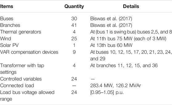
TABLE 2. System model summary.

4.1.1 Minimization of Cost Without Valve Point Effect

Generally, the cost function is quadratic and the cost curve is plotted in between real power (MW) and fuel cost ($/hr). Similarly, the objective function for cost minimization without valve point is presented as

$O{F}_{cost}=\sum _{i=0}^{NG}(a_i+b_i{P}_{gi}+c_i{P}_{gi}^2)\$/hr,(6)$

where OF_cost represents the cost in $/hr. a_i, b_i, and c_i are cost coefficients of thermal generators, listed in Table 3.

TABLE 3

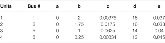
TABLE 3. Cost coefficients of single-fuel generators (Biswas et al., 2018).

4.1.2 Minimization of Cost With Valve Point Effect

The cost function as a function of valve point effect can be expressed as

$O{F}_{cos{t}_{vp}}=\sum _{i=0}^{N_g}(a_i+b_i{P}_{gi}+c_i{P}_{gi}^2|d_i\times sin(e_i\times (P_{gi}^{min}-P_{gi}))|)\$/h,(7)$

where a_i, b_i, c_i, d_i, and e_i are again the cost coefficients with valve point effect and $P_{gi}^{min}$ is the minimum power limit on the ith generator.

4.1.3 Minimization of Cost for Multi-Fuel Thermal Generators

In a power system, each generation station has different fossil fuels to produce electricity, e.g., coal, gas, and oil. The generation station with multi-fuel has a piece-wise quadratic relationship between power and cost, and the number of pieces depends on the type of fuel used. The cost of the ith generator considering multi-fuel is expressed as

$O{F}_{multi}=a_{ik}+b_{ik}{P}_{Gi}+c_{ik}{P}_{Gi}^2\$/hforfuel\prime k\prime (8)$

where k is the type of fuel such as diesel, natural gas, or heavy furnace oil. In this work, there are two generators considered multi-fuel and remaining one has a single-fuel function as explained earlier. Cost coefficients for single-fuel generators are given in Table 3 and those for multi-fuel generators are given in Table 4, whereas the precise meaning of Eqs. 6–8 is given in Ilyas et al. (2020a)

TABLE 4

TABLE 4. Cost coefficients for A and B fuels (Biswas et al., 2018).

4.2 VES Cost Model

In a power system, VESs are generally owned by private bodies. They sell power to the utility under a predefined contract. Therefore, the control and operation of VESs are in the hands of private bodies. In contrast to the conventional generation sources, VESs do not require any fuel to produce electrical energy as they utilize wind speed or sunlight to produce electrical energy which is freely available in nature. However, these private bodies charge some operation and maintenance cost to run their plants (Wijesinghe and Lai, 2011). The cost of electricity generation from these VESs mainly comprises direct cost, reserve cost, and penalty cost. The direct cost for wind and the solar plant can be calculated as in Biswas et al. (2017) and given as

$C_w(P_w)=g_w{P}_w,(9)$

$C_{pv}(P_{pv})=h_{pv}{P}_{pv},(10)$

where P_w and P_PV represent the scheduled output power from the wind farm and solar photovoltaic, respectively, and g_w and h_pv represent direct cost coefficients of VESs. As the VESs are weather dependent and due to the variable patterns of wind speed and solar irradiance, there is always uncertainty associated with the production of electricity generation from VESs. This intermittency of VESs makes it difficult to schedule generation sources. Hence, the burden on the power system operator (SO) increases in terms of optimal scheduling of its generation sources. Moreover, this variability increases the operational cost of electricity production as it becomes compulsory for the system operator to have reserve generation capacity to balance the natural fluctuations of VESs. This also introduces some computational difficulty to calculate the aggregated cost of electricity generation in OPF. Therefore, reserve and penalty cost models are introduced and integrated with the cost function in mathematical modeling as presented by Reddy et al. (2014).

Def. 3. Cost in case of overestimation: If the available power from a VES is less than the contractually agreed scheduled power, then the reserve cost model for wind power can be stated as

$C_{W_{R,i}}(\mathrm{\Delta }P)=k_{rw,i}(\mathrm{\Delta }P),(11)$

$\mathrm{\Delta }P=P_{Wsh,i}-P_{Wav,i},(12)$

where P_Wsh,_i and P_Wav,_i represent scheduled and available power capacities from a wind power source, respectively, and k_rw,_i represents the reserve cost coefficient for wind.

Def. 4. Cost in case of underestimation: In contrast to the above stated case, if the available power exceeds the scheduled power, then the system operator (SO) will pay a penalty as per the following cost model:

$C_{W_{P,i}}(\mathrm{\Delta }P)=k_{Pw,i}(\mathrm{\Delta }P),(13)$

$\mathrm{\Delta }P=P_{Wav,i}-P_{Wsh,i},(14)$

where k_Pw,_i denotes the penalty cost coefficient for the ith windmill. Similarly, the reserve and the penalty cost of solar can be calculated. Cost coefficients used in this study are given in Table 5. The reserve and penalty cost for wind and the solar plant can be calculated as in Biswas et al. (2017) and given in Eqs. 11–14. Finally, the cumulative objective function to minimize the cost is given as

$\begin{array}{ll}\hfill \mathbf{m}\mathbf{i}\mathbf{n}(f_{cost})& =f_{cos{t}_i}+[C_w(P_w)+C_{PV}(P_{PV})]+[C_{W_{R,i}}(△P)+C_{P{V}_{R,i}}(△P)]\hfill \\ \hfill & +[C_{W_{P,i}}(△P)+C_{P{V}_{p,i}}(△P)]\$/h,\hfill \end{array}(15)$

where $f_{cos{t}_i}$ is the cost of the ith thermal generator which may be single fuel and multi-fuel. The second term represents the direct cost of wind and solar. The third term represents the reserve cost of wind and solar, and the fourth term represents the penalty cost of wind and solar.

TABLE 5

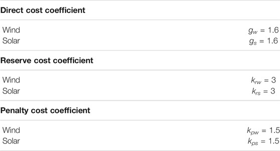
TABLE 5. Cost coefficients for RESs (Biswas et al., 2017).

4.3 Equality Constraints

• The nodal active power balance at the ith bus is given as follows:

$P_{Gi}-P_{Di}=V_i\sum _{j=1}^{NB}{V}_j[G_{ij}cos({\delta }_{ij})+B_{ij}sin({\delta }_{ij})],i\in N.(16)$

• The nodal reactive power balance at the ith bus is given as

$Q_{Gi}-Q_{Di}=V_i\sum _{j=1}^{NB}{V}_j[G_{ij}cos({\delta }_{ij})+B_{ij}sin(\delta ij)],i\in N,(17)$

where elements of the admittance matrix are calculated as

$Y_{ij}=G_{ij}+B_{ij}.(18)$

Equality constraints shown in Eqs. 16–18 are thoroughly discussed by Chen et al. (2018). The convergence process of load flow will not violate the equality constraint limits eventually.

4.4 Inequality Constraints

• Real power limits of generation sources including maximum penetration of wind and solar can be written as

$P_{Gi}^{min}\le P_{Gi}\le P_{Gi}^{max}\forall i=\mathrm{1,2},\dots ,NG.(19)$

• Reactive power limits of generation sources can be written as

$Q_{Gi}^{min}\le Q_{Gi}\le Q_{Gi}^{max}\forall i=\mathrm{1,2},\dots ,NG.(20)$

• Voltage limits of generator buses are given as

$V_{Gi}^{min}\le V_{Gi}\le V_{Gi}^{max}\forall i=\mathrm{1,2},\dots ,NG,(21)$

where NG is the total number of thermal generators, wind and solar plant.

• The line thermal limit of all branches is given as

$P_{ij}<T{L}_{ij},(22)$

where TL_ij gives the thermal limit of the power flow line from node i to j.

• For the secure operation of the power system, it is compulsory to maintain the load bus voltages within the allowable range. Load bus voltage limits are given as

$V_{Li}^{min}\le V_{Li}\le V_{Li}^{max}\forall i=\mathrm{1,2},\dots ,NG.(23)$

The specific meaning of each variable in Eqs. 19−23 is well explained by Chen et al. (2018). Feasible values of control or independent variables among the inequality constraints are selected by the optimization algorithm within their allowable boundaries. An effective constraint handling technique to pick the feasible values of state or dependent variables is discussed in Section IV-E.

4.5 Constraint Handling Approach

While using an evolutionary algorithm (EA) to solve an optimization problem, it is important to use a proper constraint handling approach (CHA). An EA equipped with a proper CHA can guide the search process toward a globally feasible solution. CHAs are able to use the information hidden in infeasible solutions, and hence, they do not discard any infeasible solution immediately by Tessema et al. (2006). Deb (2000a) proposed an efficient method to handle the constraint diversification. Equality constraints are converted to inequality constraints by introducing the tolerance factor δ in equality constraints. The ultimate constraint violation for an infeasible solution is calculated as in Biswas et al. (2018) and Deb (2000b) and given in Eqs. 24, 25:

$K(X)=\frac{\sum _{j=1}^N{w}_h\left(G_i(X)\right.}{\sum _{j=1}^N{w}_h},(24)$

where w_h is the weighting parameter for constraint violation, and

$w_h=\frac{1}{G_{i,max}},(25)$

where G_i, max is the maximum value of constraint violation from the G_i(X) set. Consequently, equality constraints in three are converted into inequality constraints. A brief description of CHA is presented in the next section.

4.5.1 SF

In the SF approach, two fitness values of the objective function (X_i, X_j) are always compared to each other, and a decisive logic is used to discard the less feasible value. The algorithmic logic to pick a superior solution is explained in Algorithm 1.

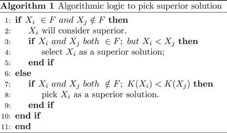
The SF approach always picks a feasible solution when other belongs to the infeasible search space. On the contrary, a solution having a smaller fitness value has been picked when both belong to a feasible region F. Similarly, a solution with the lowest overall constraint violation K(X) in Eq. 24 has been picked when both do not belong to the feasible space F. That is how this approach pushes infeasible solutions toward feasible space and converges the search process to an optimal solution.

5 VES Models

5.1 Wind Generator Model

In this work, a wind farm that has 25 wind turbines is associated with transport 13, as demonstrated in Figure 1. Every turbine has 3 MW appraised power. In any case, the accessible power got from a wind farm differs from the wind speed. Along these lines, to compute the accessible genuine power, the model introduced by Biswas et al. (2017) is utilized. The yield power of a wind turbine relies upon wind speed and can be numerically communicated through Eq. 26 taken from Biswas et al. (2017):

$P_w(v)=\left\{\begin{array}{cc}0\hfill & \text{for}v<v_{in}\&v>v_{out}\hfill \\ p_{wr}\left(\frac{v-v_{in}}{v_r-v_{in}}\right)\hfill & \text{for}{v}_{in}\le v\le v_r\hfill \\ p_{wr}\hfill & \text{for}{v}_r<v\le v_{out},\hfill \end{array}\right.(26)$

where p_wr is the rated power of the wind turbine and v, v_r, v_in, v_out are the actual and rated speed and cut-in and cut-out speed, respectively. The rated values are considered as v_r = 16 m/s, v_in = 3 m/s, and v_out = 25 m/s.

FIGURE 1

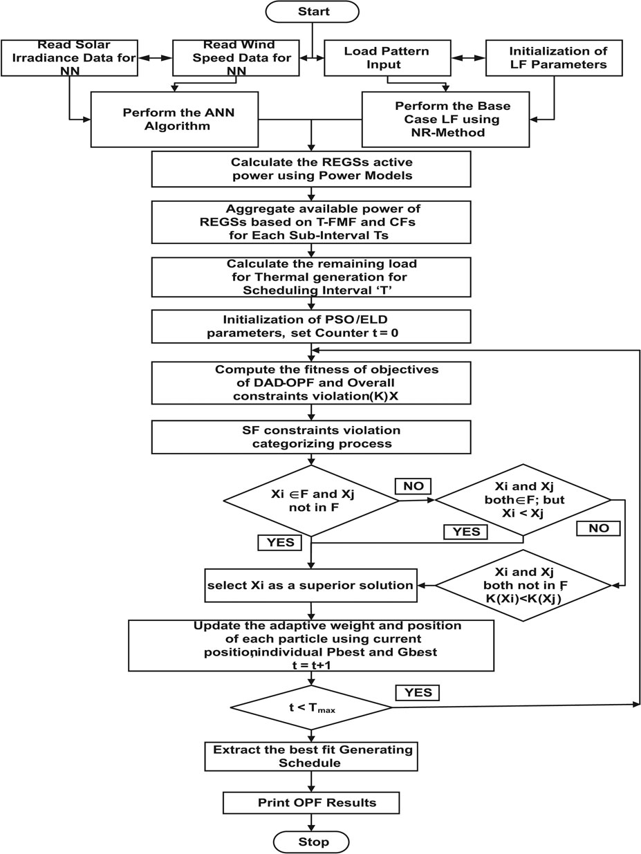
FIGURE 1. IEEE 30-bus system model.

5.2 Model of Photovoltaic Generation

5.2.1 Power Model

For the solar power, the energy conservation model given by Biswas et al. (2017) is expressed through the following equation:

$P_s(G)=\left\{\begin{array}{cc}{P}_{sr}\frac{G^2}{G_{std}{R}_c}\hfill & \text{for}0\le G\le R_c\hfill \\ P_{sr}\frac{G}{G_{std}}\hfill & \text{for}G\ge G,\hfill \end{array}\right.(27)$

where G, G_std, R_c, and P_sr are forecasted solar radiation, solar radiations at STP, actual solar irradiation, and rated output power, respectively. In simulations, G_std = 800 W/m², R_c = 120 W/m² are considered.

6 Wind and Solar Forecasting Model

As the VESs are intermittent, the variability of the available power from these sources poses a challenge to meet the variable load demand of the power system. Therefore, it is important to predict the wind speed and solar irradiance before scheduling the generation sources. For this purpose, the ANN is used to predict wind speed and solar irradiance. The details are given below.

6.1 Fundamentals of ANN

In energy engineering systems, the ANN is being used extensively for modeling and prediction purposes. The requirement to set up an ANN is the historical datasets. In the case of weather forecasting, historical data can be collected by using sensors, which can continuously monitor and record different attributes of weather. The meteorological data used in this paper are collected during the period from January 1, 2015, to December 31, 2017, from Danyore Weather Station (DWS) at Hunza, Pakistan, and Lahore Weather Station (LWS) at Lahore, Pakistan. Different algorithms are used to predict wind speed and solar irradiance by using the ANN. The basic ANN equation to map the output Yvia a non-linear input feature vector X given in Eq. 28 is taken from Quej et al. (2017). The architecture diagram of the presented ANN is given in Figure 2. However, for the backpropagation error minimization, the LM algorithm is finally adopted because it is efficient in handling errors in shallow networks. The details of this algorithm are given below.

$Y=f(X)=X^{T}w+b.(28)$

FIGURE 2

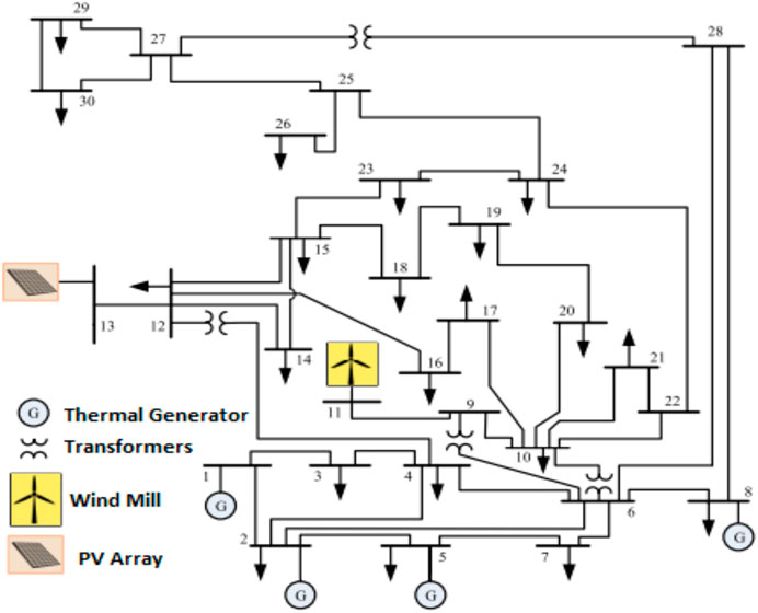
FIGURE 2. Architecture of the NN.

6.1.1 LM Algorithm

This algorithm uses two numerical minimization methods: gradient descent and Gauss–Newton. The former algorithm is based on backpropagation (BP) training of the NN. It has been widely used in weather forecasting because of its ability to model non-linear separable problems by Qazi et al. (2015). In the latter method, the sum of squared errors is minimized by assuming that the least-squares function is locally quadratic in the parameters and finding the minimum of this quadratic. When the parameters are found far away from the feasible value, the LM method adopts the gradient-descent method. On the contrary, the Gauss–Newton method is opted when the parameters are found near the feasible value. The LM algorithm modifies the parameter updates, and the update function U(k) can be computed using Eq. 29 given in Qazi et al. (2015):

$U(k)=-{\left[J^T\times J+\beta \times I(J^T\times J)\right]}^{-1}\times J^T\times \epsilon ,(29)$

where first-order derivatives of the network errors for the weights and biases are included in a Jacobian matrix J, ɛ is the network error vector, β is a non-negative scalar number called the damping factor, and I is a diagonal identity matrix. The performance parameters used for the LM algorithm are given in Table 6. The values of these parameters are selected as default settings by the NN tool of Matlab program.

TABLE 6

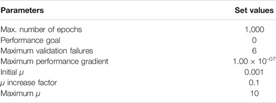
TABLE 6. LM algorithm parameters.

7 The Proposed DA-DOPF Approach

7.1 Overview of the Proposed Approach

Recently, numerical optimization techniques are used in the development of EA, which are population-based and a potential candidate to solve optimization problems, and can efficiently avoid the problems of classical methods, e.g., lack of convergence or step size issues. PSO has been used in many power flow studies to solve OPF because of its efficient population-based heuristic nature and flexible and well-balanced approach of global and local exploration (Abido, 2002c). Moreover, scheduling and planning of power systems having VESs is a difficult task due to the unpredictable available power of VESs. It is worth mentioning here that many researchers have used ANNs for weather forecasting to estimate the generated power of VESs in the smart grid (Moghaddam and Seifi, 2011). This study is carried out to solve a DA-DOPF problem for a power system having renewable energy sources. The main objective of this study is to schedule the generation sources at optimal values so that the cost of electricity generation remains at its minimum value, with the satisfaction of OPF constraints as explained earlier in Section IV. The said objective is achieved by using the PSO/ELD algorithm in conjunction with the ANN which is used to forecast the solar radiation and wind speed pattern on an hourly basis to calculate the available power of VESs. Moreover, the developed technique is equipped with an effective constraint handling approach to handle the violation of inequality constraints. Therefore, to handle the diversification of these inequality constraints, the SF constraint handling technique is used. Hence, the proposed approach differs from other available approaches found in the literature regarding violation of equality constraints on dependent variables (Surender Reddy and Bijwe, 2016; Grover-Silva et al., 2018). Moreover, the 1-h interval is divided into fifteen sub-intervals to achieve the dynamic generation schedule. It is worth mentioning here that the idea of using T-FMF to calculate CFs is never used before which provides the sub-interval variation of VESs and makes it easy to analyze the setting of control variables.

7.2 PSO

Numerical optimization has the ability to overcome convergence or step size problems in classical optimization techniques. PSO has been used in many power flow studies to solve OPF because of its efficient population-based heuristic nature and flexible and well-balanced approach of global and local exploration by Abido (2002c). Moreover, scheduling and planning of power systems having VESs is a difficult task due to the unpredictable available power of VESs. It is worth mentioning here that many researchers have used ANNs for the purpose of weather forecasting to estimate the generated power of VESs in the smart grid (Moghaddam and Seifi, 2011).

This study is carried out to solve a DA-DOPF problem for a power system having renewable energy sources. The main objective of this study is to schedule the generation sources at optimal values so that the cost of electricity generation remains at its minimum value, with the satisfaction of OPF constraints as explained earlier in Section IV. The said objective is achieved by using the PSO-economic load dispatch (ELD) algorithm in conjunction with the ANN which is used to forecast the solar radiation and wind speed pattern on an hourly basis to calculate the available power of VESs. Moreover, the developed technique is equipped with an effective constraint handling approach to handle the violation of inequality constraints. Therefore, to handle the diversification of these inequality constraints, the SF constraint handling technique is used. Hence, the proposed approach differs from other available approaches found in the literature regarding violation of equality constraints on dependent variables (PSO is a nature-inspired optimization algorithm that starts with the random initialization of solutions). This swarm of solutions moves with a randomized velocity within the search space. Each solution of this swarm is known as a particle. Every particle remembers its last position in the search space to achieve the best position. The objective function fitness value at this position is saved as “pbest.” To achieve the most optimal fitness value, the position of a global version of the swarm is saved as “gbest” which is the overall minimum value of objective function achieved at the present iteration of the algorithm loop. Before the next search iteration, the velocity of every particle is updated so that the swarm moves toward the global best value. Basic elements and mathematics of this algorithm are briefly stated and defined as follows:

Particle, X(t): It represents a solution of the m-dimensional vector, where the number of optimized parameters is given by m. Each search point is known as a particle. The value of the objective function for X(t) can be a possible solution. The position of X(t) can be influenced by different optimized parameters.

Population, pop(t): It is a set of n particles which is known as the population of size n. At each iteration t, the population vector can be written as $pop(t)={[X_1(t),\dots ,X_n(t)]}^T$.

Particle velocity, V(t): The particles are directed to be moving with velocity V_j(t) within the search space. This movement is responsible to find the optimal value of the objective function. At every generation, each particle can be assigned an updated velocity to move within the search space given in the following equation as explained by Surender Reddy and Bijwe (2016) and Grover-Silva et al. (2018):

$V_i^{t+1}=V_i^t+c_1{U}_1^t(p{b}_i^t-X_i^t)+c_2{U}_2^t(g{b}^t-X_i^t),(30)$

where $V_i^t$ is the initial velocity; $p{b}_i^t-X_i^t$ is the self-influence; $g{b}^t-X_i^t$ is the global influence; c₁ is called the cognitive parameter and c₂ is called the social parameter, which both are called acceleration coefficients; and $U_1^t$ and $U_2^t$ are two random numbers that vary between 0 and 1 and the position is updated according to the following expression:

$X_i^{t+1}=X_i^t+V_i^{t+1}.(31)$

Inertia weight, w(t): To influence the moving capabilities of a particle inertia weight, w(t) is used. Global exploration capabilities of the algorithm can be enhanced at the start by assigning a large inertia weight. In contrast, at the end of the search process, they can be reduced to improve the local search ability of a particle. The inertial weight reduction can be achieved by using an annealing decrement function as follows:

$w(t)=\alpha w(t-1),(32)$

where α is a decrement constant and its value is less than 1. While solving for minimization problems, the personal best pb_i at iteration t + 1 is calculated as

$p{b}_i^{t+1}=\left\{\begin{array}{cc}p{b}_i^t\hfill & \text{if}f(X_i^{t+1})>p{b}_i^{t+1}\hfill \\ p{b}_i^t\hfill & \text{if}f(X_i^{t+1})\le p{b}_i^{t+1},\hfill \end{array}\right.(33)$

where f: F_n → F is the fitness function. The global best position gb in each algorithm loop t is calculated as

$gb=min[p{b}_i^t],(34)$

where i ∈ pop(t). Here, it is important to note that, at every iteration, each particle knows its personal best “pb” and remembers this value till the next iteration. While at the time “t,” the overall minimum value of swarm is known as the global best position “gb.” In the next loop, updated velocities and positions are assigned to each particle of the swarm. Now to calculate the fitness of objective function, these particle positions are used. In this algorithmic flow, the minimum fitness value achieved by the entire swarm is called new gbest, and the minimum fitness value is achieved by the particle itself and is called new pbest. This process repeats until the user-defined stopping criteria (limitation of maximum iteration) are satisfied. The control parameters used for the PSO algorithm are given in Table 7. The values of these parameters are selected by a training algorithm with different patterns of parameters and fine-tuning.

TABLE 7

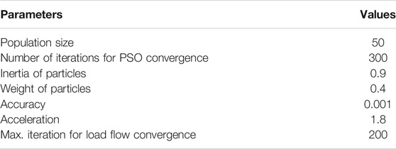
TABLE 7. Control parameters of the PSO algorithm.

7.3 T-FMF

The contributing factors (CFs) for VESs are calculated by using T-FMF which is derived from the fuzzy decision-making approach. Hence, variation in the real power of VESs during the sub-interval is realized by the use of T-FMF; in this way, CFs are calculated at the start of the algorithm loop, which helps to inspect the variation in real power loss and overall cost of the network. Moreover, the proposed technique is capable of calculating the most economical generation schedule by assigning CFs to VESs. Therefore, generation cost is kept at its minimum value along with the reduction in line loss of the system. The FMF values μ for RES contributions are computed and defined as in Ilyas et al. (2020a) by the following equation:

${\xi }_j(c{f}_j)=\left\{\begin{array}{cc}0\hfill & \text{for}c{f}_j\le y_1\hfill \\ (c{f}_j-y_1)/(y_2-y_1)\hfill & \text{for}{y}_1<c{f}_j<y_2\hfill \\ 1\hfill & \text{for}c{f}_j\ge y_2.\hfill \end{array}\right.(35)$

Here, cf_j shows the value of CF. In this work, y₁ and y₂ are considered as 0 and 1.25, respectively, as given by Kaur and Jain (2017), while the aggregated real power from VESs is expressed through the following equation:

$VES{s}_{TP}=\{{\xi }_w\times P_w\}+\{{\xi }_{pv}\times P_{pv}\}.(36)$

7.4 Computational Flow

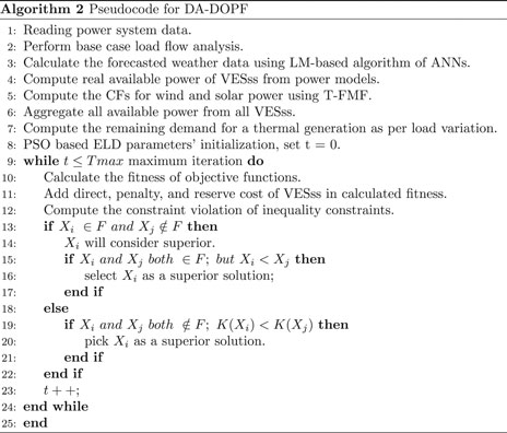
As has been discussed in the earlier sections, the intermittency of VESs in electricity generation introduces a challenge to develop an efficient DA-OPF program. All the available approaches in the literature can handle this challenge effectively. Therefore, this paper proposed a technically and computationally efficient approach to solve the DA-OPF problem. The computational flow starts from the prediction of solar intensity and wind speed pattern which is used in the calculation of available power from VESs. Then, CFs are calculated using T-FMF to consider the dynamic behavior of VESs. The variable load pattern is assumed to be available at the start of the DA-DOPF loop. Therefore, the remaining load is being calculated which is beyond the available generation capacity of VESs. Furthermore, thermal generators are scheduled at the optimal values to cater to the remaining load. In addition, the SF constraint handling approach is used to avoid the constraint violation referring to the limits of the dependent variables. In the end, a confident and global feasible solution is achieved from the search space. The computational flow of the proposed approach is further elaborated in Algorithm 2. Moreover, continuity of the steps is represented pictorially in Figure 3.

FIGURE 3

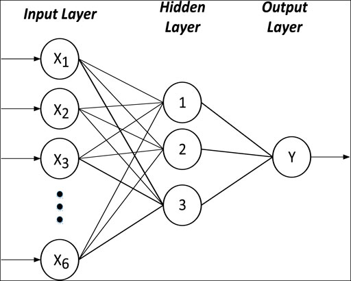
FIGURE 3. DA-DOPF flow chart.

7.5 System Model

In this work, for understanding and analyzing solar and wind, the standard IEEE 30-bus system of 41 branches is used and VESs are integrated at different buses. A 75 MW wind farm is inserted at bus 11 having 25 wind turbines each of 3 MW. Similarly, a solar PV plant of capacity 60 MW is integrated at 13. Moreover, bus 1 is taken as a slack bus, and at buses 2, 5, and 8, conventional thermal generators are placed. The maximum connected load at once is assumed to be 283.4 MW. Furthermore, a variable load is assumed to be available at every hour. The amended system model is shown in Figure 1. The summary of the IEEE 30-bus system model is given in Table 2. Nevertheless, the proposed approach is generic such that it can be easily implemented on any system model with more buses.

7.6 Climatic Data Representation in 1D and 2D

Meteorological data are smartly classified in 2D arrays as given in Eqs. 37, 38. In data matrices, the row shows the number of days in a month and column shows the number of hours in a day. Here, each element represents the measured value of solar irradiance and wind speed. To show the periodic nature of solar irradiance, meteorological data are plotted in a 2D plot in Figure 4. Similarly, the stochastic nature can be analyzed by a 2D plot of wind data in Figure 5. The variable nature of solar irradiance and wind speed in a single day is shown in a 1D plot in Figure 6.

$Solar-Ir{r}_{(D,H)}=\left(\begin{array}{cccc}\hfill r_{\mathrm{1,1}}\hfill & \hfill r_{\mathrm{1,2}}\hfill & \hfill \cdots \hfill & \hfill r_{\mathrm{1,24}}\hfill \\ \hfill r_{\mathrm{2,1}}\hfill & \hfill r_{j,k}\hfill & \hfill \cdots \hfill & \hfill r_{\mathrm{2,24}}\hfill \\ \hfill ⋮\hfill & \hfill ⋮\hfill & \hfill \ddots \hfill & \hfill ⋮\hfill \\ \hfill r_{\mathrm{31,1}}\hfill & \hfill r_{\mathrm{31,2}}\hfill & \hfill \cdots \hfill & \hfill r_{\mathrm{31,24}}\hfill \end{array}\right),(37)$

$Wind-Spee{d}_{(D,H)}=\left(\begin{array}{cccc}\hfill v_{\mathrm{1,1}}\hfill & \hfill v_{\mathrm{1,2}}\hfill & \hfill \cdots \hfill & \hfill v_{\mathrm{1,24}}\hfill \\ \hfill v_{\mathrm{2,1}}\hfill & \hfill v_{j,k}\hfill & \hfill \cdots \hfill & \hfill v_{\mathrm{2,24}}\hfill \\ \hfill ⋮\hfill & \hfill ⋮\hfill & \hfill \ddots \hfill & \hfill ⋮\hfill \\ \hfill v_{\mathrm{31,1}}\hfill & \hfill v_{\mathrm{31,2}}\hfill & \hfill \cdots \hfill & \hfill v_{\mathrm{31,24}}\hfill \end{array}\right),(38)$

where r_j,_k, v_j,_k represent the solar irradiance and wind speed of the jth day at kth hour.

FIGURE 4

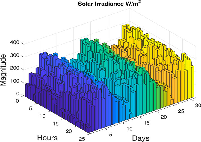
FIGURE 4. Solar data in a 2D plot.

FIGURE 5

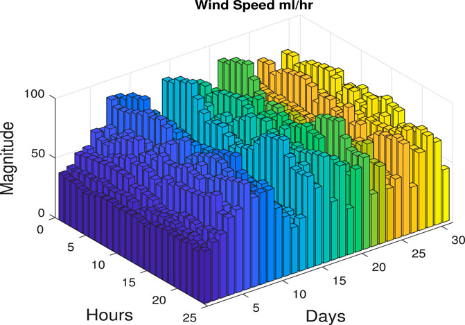
FIGURE 5. Wind data in a 2D plot.

FIGURE 6

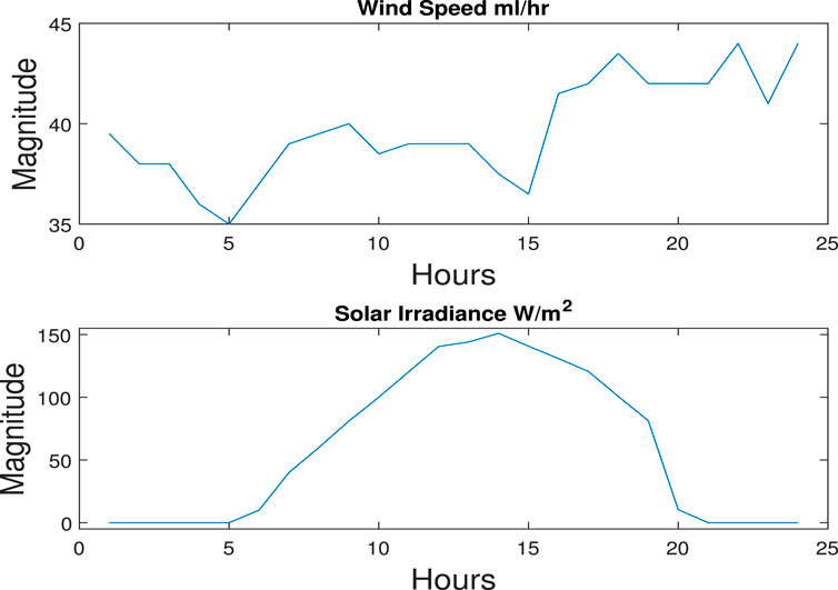
FIGURE 6. Wind and solar data in 1D plots.

j_(Days) = 1, 2, …., 31

k_(Hours) = 1, 2, …., 24.

8 Results and Discussions

8.1 Forecasting Performance Evaluation

The accuracy of the ANN models is analyzed based on the maximum prediction error (MPE) and root mean square error (RMSE). However, various training algorithms are tested. During the trial process, the algorithms are compared based on RMSE and resemblance of predicted values to target values. Comparison of different algorithms suggests that the LM algorithm performs better than others on the input data; therefore, it is adopted for the training phase of the network. Besides, it is tracked down that the eight neurons in the hidden layer related to the LM preparing calculation give the best presentation and the least forecast error. In Figure 7, the performance curve of solar irradiance is plotted against epochs, and it has been found that desired results are obtained at the 171st epoch. Similarly, for wind in Figure 8, it can be noticed that the best results are achieved after 1,000 epochs because of a large number of parameters and sparseness in the data. Furthermore, regression plots of solar and wind generation are shown in Figures 9, 10, respectively. It is obvious from these plots that the NN is well trained and data are well fit during all phases of the algorithm. Furthermore, to highlight the superiority of the LM algorithm to some other algorithms, the RMSE is presented in Table 8. It can be noticed that the least error has been achieved by the proposed algorithm.

FIGURE 7

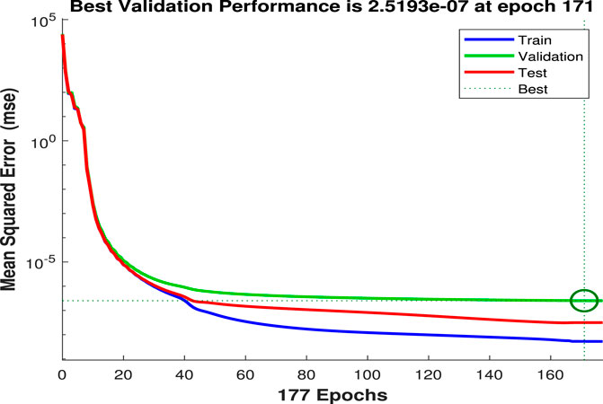
FIGURE 7. Solar performance.

FIGURE 8

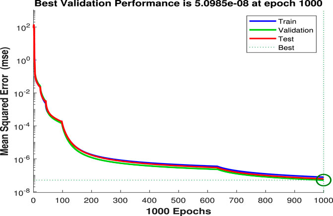
FIGURE 8. Wind performance.

FIGURE 9

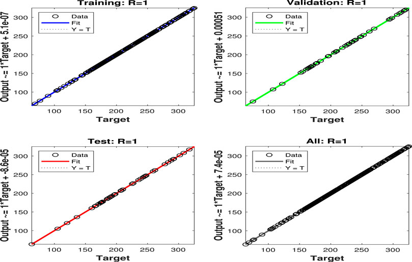
FIGURE 9. Solar regression.

FIGURE 10

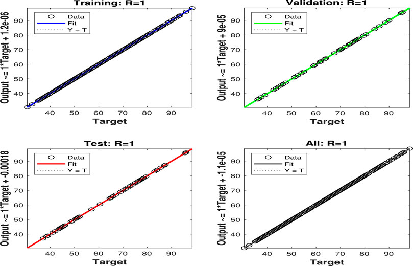
FIGURE 10. Wind regression.

TABLE 8

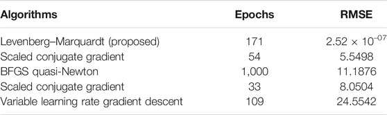
TABLE 8. RMSE comparison.

8.2 Performance Evaluation of Proposed DA-DOPF

The DA-DOPF optimized Eq. 15 represents that the scheduling period considered in this study is 1 h which is further divided into six sub-intervals of 10 min. Therefore, by keeping in mind the intermittent nature of VESs, it is considered in this work that the proposed DA-DOPF is performed every 10 min for the dynamic dispatch of generation sources. Moreover, optimizing energy for each hour and optimal generation cost are calculated for (24 × 10) sub-intervals based on CFs of VESs. The contribution of thermal generators and VESs in these sub-intervals is shown in the bar chart plotted in Figure 11. Table 9 shows the optimal contribution of generation sources (GSs) along with voltages and reactive power settings. Furthermore, the optimized cost for sub-intervals is also presented in Table 9 which is calculated using the PSO-based optimization ELD program. As per predicted values of solar irradiance and wind speed, available VES power is calculated. Penalty and reserve costs for wind and solar are computed using Eqs. 11, 13, respectively. In addition, to consider the variable nature of the connected load, the varying load pattern for 24 h is shown in Figure 12. Therefore, the cumulative basic cost with valve point effect and cost with multi-fuel are calculated in multiple runs of the algorithm. Consequently, the convergence plot of PSO for this optimization problem is shown in Figure 13, where the x-axis shows the number of iterations and the optimal value of the objective function (overall cost) is found at the 60th epoch of the algorithm. However, detailed numerical analysis is presented subsequently.

FIGURE 11

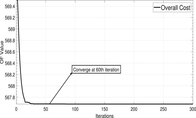
FIGURE 11. Contribution of GSs in sub-intervals.

TABLE 9

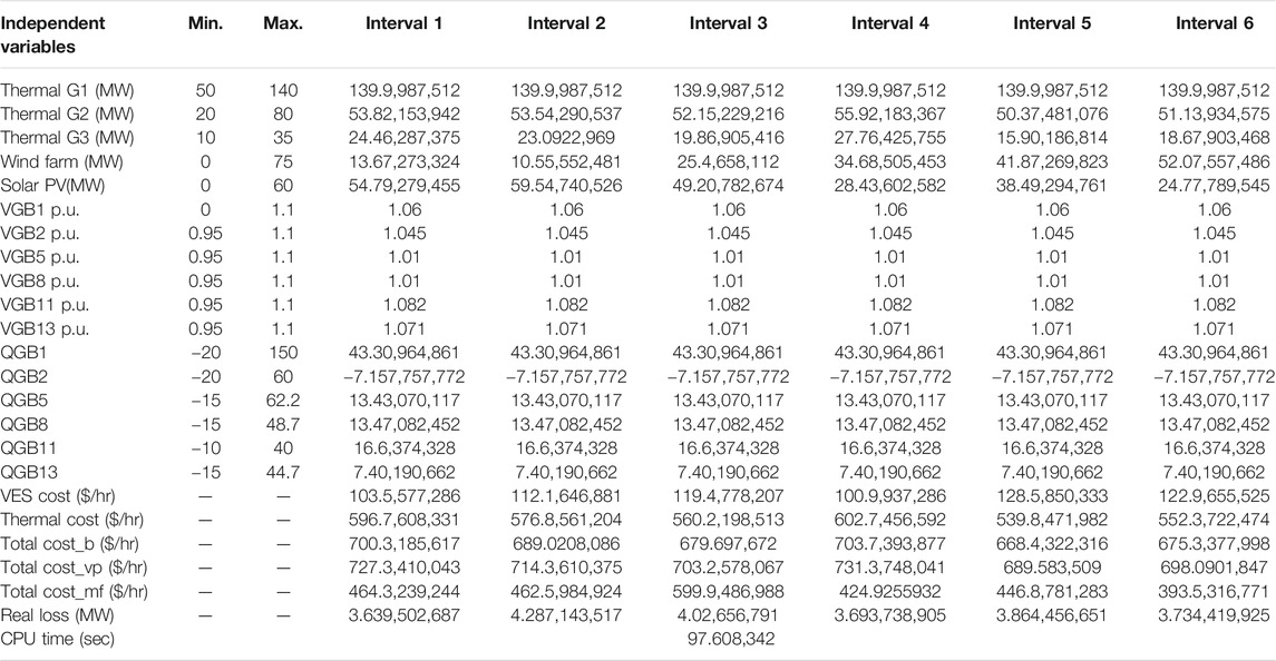
TABLE 9. Independent variable settings for DA-DOPF.

FIGURE 12

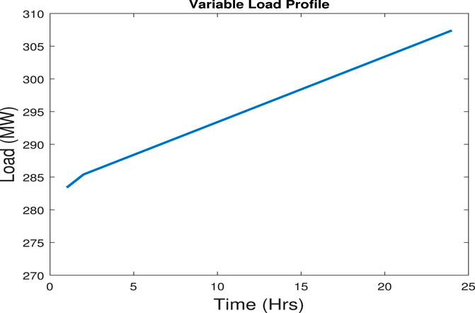
FIGURE 12. Variable load pattern.

FIGURE 13

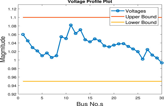
FIGURE 13. Convergence characteristics.

8.2.1 Numerical Result Comparison

This sub-section presents the comparison of numerical results while optimizing the cost for DA-DOPF. Dependent (state) variables are listed column-wise in Table 9 with their boundary limits. In addition to this allowable limit of the dependent and independent variables, bus data and branch data considered in this study are taken from Zimmerman and Murillo-Sánchez (2016). During the optimization algorithm, the active and reactive power of all generation sources and voltages of generator buses are considered constraints. Additionally, the SF constraint handling technique is used to handle the constraint violation for these variables. The effectiveness of the CH technique can be seen from the listed values of these variables for a different interval of DA-DOPF. Moreover, the approximated (CPU) time of the algorithm run is given in Table 9. Furthermore, a comparison of the presented approach with some previously mentioned techniques is given in Table 10. The main advantage of the SF constraint handling approach can be noticed from this comparison. It utilizes the information hidden in the infeasible solution and does not discard it straight away. Therefore, the solution found by the proposed technique is most optimal, and the reduction in generation cost is noticeable. Moreover, it is worth mentioning here that the proposed approach is compared based on the constraint handling techniques in conjunction with different optimization algorithms. Furthermore, it is also compared with some multi-objective optimization cases. Yet, in all these comparisons, the proposed approach is found best, and the values of basic cost, cost with multi-fuel, and system loss are presented column-wise in bold text. For Interval 6 of optimizing basic fuel cost, DA-DOPF/SF algorithms lead to fuel costs of 675.33 $/h. It is important to explain here that the on front of the inequality constraint of generator reactive power and load bus voltage, presented results are satisfactory and operating voltages of all buses of the IEEE 30-bus system remain within their allowable limits. The voltage profile of the system is plotted in Figure 14. A cursory glance at the voltage profile graph shows that most buses do not fall below the value of 1.0 p.u. On the contrary, voltages never exceed the value of 1.08 p.u. Therefore, the over-voltage problem during load management is controlled through the proposed constraint handling technique. Hence, the faithful operation of the power system is assured without any voltage stress for connected load at the PQ buses.

TABLE 10

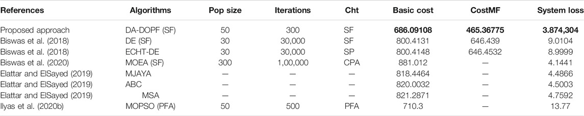
TABLE 10. Comparison with existing techniques. Cht = constraint handling technique. Basic and other cost are calculated in = $/h. System loss is calculated in MW (mega watts).

FIGURE 14

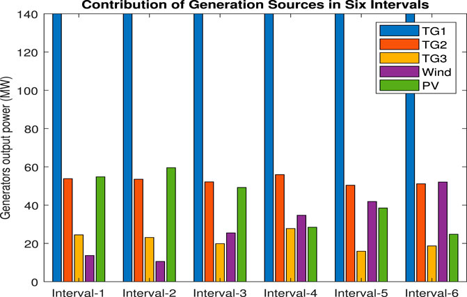
FIGURE 14. Voltage profile.

9 Conclusion

In the previously presented studies, conventional day-ahead optimal power flow (CDA-OPF) and real-time optimal power flow (RT-OPF) approaches did not cover the effects of the integration of VESs. Additionally, the variability of available power introduces the additional challenge to consider the scenarios of over- and underestimation. On the contrary, constraint violation techniques are also not considered in the available literature. Therefore, in this study, the day-ahead dynamic optimal power flow (DA-DOPF) problem is carried out with effects of intermittency of VESs. Moreover, to handle the constraint violation, the SF constraint handling technique is used. Therefore, an infeasible solution was not discarded straight away. Hence, a more confident and optimal solution is computed using the optimization program based on the PSO algorithm. In addition to this, the proposed approach is combined with the NN-based prediction model which is used to forecast day-ahead wind and solar irradiance. Moreover, T-FMF calculates the membership value of VESs in the synergy of generation. Hence, DA-DOPF has been run for the six sub-intervals, and an optimal generation schedule is computed while ensuring the physical and security limits of the power system. Finally, the proposed approach is tested for an amended IEEE 30-bus system. The optimization program is coded in MATLAB 2018a and uses the MATPOWER toolbox for computing load flow. Consequently, results obtained from these simulations are presented in tabular form as well as in graphical plots. However, the approach is quite different from the available literature, yet the comparison is done based on minimum generation cost and real loss. It is worth mentioning here that the presented approach was found superior in numerical analysis to the other similar approaches.

Nevertheless, the authors suggest the future scope with the induction of more renewable energy sources, MPPT for solar arrays, battery storage system, and more number of buses in the power system, as well as future scope in the integration of FACT devices and optimal placement of distributed generation sources and FACT devices.

Data Availability Statement

The datasets presented in this study can be found in online repositories. The names of the repository/repositories and accession number(s) can be found below: IEEE Standard Bus System.

Author Contributions

MI, MA, and MR gave the problem statement, formulated the problem, and implemented the proposed approach. MR, TA, and AM reviewed the paper and supervised the work.

Funding

This project was funded by the Deanship of Scientific Research (DSR) at King Abdulaziz University, Jeddah, under grant number RG-13-135-41. The authors, therefore, acknowledge with thanks the DSR for their technical and financial support. This project has also received funding from the European Union Horizon 2020 research and innovation programme under the Marie Sklodowska-Curie grant (agreement No. 754382), GOT ENERGY TALENT. The content of this (report/study/article/publication) does not reflect the official opinion of the European Union. Responsibility for the information and views expressed herein lies entirely with the authors.

Conflict of Interest

The authors declare that the research was conducted in the absence of any commercial or financial relationships that could be construed as a potential conflict of interest.

Publisher’s Note

All claims expressed in this article are solely those of the authors and do not necessarily represent those of their affiliated organizations, or those of the publisher, the editors, and the reviewers. Any product that may be evaluated in this article, or claim that may be made by its manufacturer, is not guaranteed or endorsed by the publisher.

References

Abido, M. A. (2002a). Optimal Power Flow Using Tabu Search Algorithm. Electric Power components Syst. 30, 5. doi:10.1080/15325000252888425

CrossRef Full Text | Google Scholar

Abido, M. A. (2002b). Optimal Power Flow Using Particle Swarm Optimization. Int. J. Electr. Power Energ. Syst. 24, 7. doi:10.1016/s0142-0615(01)00067-9

CrossRef Full Text | Google Scholar

Abido, M. A. (2002c). Optimal Power Flow Using Particle Swarm Optimization. Int. J. Electr. Power Energ. Syst. 24 (7), 563–571. doi:10.1016/s0142-0615(01)00067-9

CrossRef Full Text | Google Scholar

Abou El-Ela, A. A., and Abido, M. A. (1992). Optimal Operation Strategy for Reactive Power Control. Model. Simulation Control. A Gen. Phys. Matter Waves Electr. Electronics Eng. 41, 19.

Google Scholar

Ahn, S-H., Lee, K-T., Bhandari, B., Lee, G-Y., Caroline, S-Y., and Song, C-K. (2012). Formation Strategy of Renewable Energy Sources for High Mountain Off-Grid System Considering Sustainability. J. Korean Soc. Precision Eng. 29, 9. doi:10.7736/kspe.2012.29.9.958

CrossRef Full Text | Google Scholar

AlRashidi, M. R., and El-Hawary, M. E. (2009). Applications of Computational Intelligence Techniques for Solving the Revived Optimal Power Flow Problem. Electric Power Syst. Res. 79, 4. doi:10.1016/j.epsr.2008.10.004

CrossRef Full Text | Google Scholar

Alsac, O., and Stott., B. (1974). Optimal Load Flow With Steady-State Security. IEEE Trans. Power apparatus Syst. 3, 4. doi:10.1109/tpas.1974.293972

CrossRef Full Text | Google Scholar

Aoki, K., Nishikori, A., and Yokoyama, R. (1987). Constrained Load Flow Using Recursive Quadratic Programming. IEEE Trans. Power Syst. 2, 1. doi:10.1109/tpwrs.1987.4335064

CrossRef Full Text | Google Scholar

Baghaee, H. R., Mirsalim, M., Gharehpetian, G. B., and Talebi, H. A. (2017). Fuzzy Unscented Transform for Uncertainty Quantification of Correlated Wind/PV Microgrids: Possibilistic–Probabilistic Power Flow Based on RBFNNs. IET Renew. Power Gener. 2017, 1. doi:10.1049/iet-rpg.2016.0669

Google Scholar

Baghaee, H. R., Mirsalim, M., Gharehpetian, G. B., and Talebi, H. A. (2018). Generalized Three Phase Robust Load-Flow for Radial and Meshed Power Systems With and without Uncertainty in Energy Resources Using Dynamic Radial Basis Functions Neural Networks. J. Clean. Prod. 2018, 1. doi:10.1016/j.jclepro.2017.10.316

CrossRef Full Text | Google Scholar

Banos, R., Manzano-Agugliaro, F., Montoya, F. G., Gil, C., Alcayde, A., and Gómez, J. (2011). Optimization Methods Applied to Renewable and Sustainable Energy: A Review. Renew. Sustain. Energ. Rev. 15, 4. doi:10.1016/j.rser.2010.12.008

CrossRef Full Text | Google Scholar

Barbounis, T. G., Theocharis, J. B., Alexiadis, N. C., and Dokopoulos, P. S. (2006). Long-Term Wind Speed and Power Forecasting Using Local Recurrent Neural Network Models. IEEE Trans. Energ. Convers. 21, 1. doi:10.1109/tec.2005.847954

CrossRef Full Text | Google Scholar

Biswas, P. P., Suganthan, P. N., and Amaratunga, G. A. J. (2017). Optimal Power Flow Solutions Incorporating Stochastic Wind and Solar Power. Energ. Convers. Management. 148, 1194–1207. doi:10.1016/j.enconman.2017.06.071

CrossRef Full Text | Google Scholar

Biswas, P. P., Suganthan, P. N., Mallipeddi, R., and Gehan, A. J. (2018). Optimal Power Flow Solutions Using Differential Evolution Algorithm Integrated with Effective Constraint Handling Techniques. Engineering Applications of Artificial Intelligence.

Biswas, P. P., Suganthan, P. N., Mallipeddi, R., and Amaratunga, G. A. J. (2020). Multi-Objective Optimal Power Flow Solutions Using a Constraint Handling Technique of Evolutionary Algorithms. Soft Comput. 24 (4), 2999–3023. doi:10.1007/s00500-019-04077-1

CrossRef Full Text | Google Scholar

Burchett, R. C., Happ, H. H., and Vierath, D. R. (1984). Quadratically Convergent Optimal Power Flow. IEEE Trans. Power Apparatus Syst. 11, 3267. doi:10.1109/tpas.1984.318568

CrossRef Full Text | Google Scholar

Cao, J. C., and Cao, S. H. (2006). Study of Forecasting Solar Irradiance Using Neural Networks with Preprocessing Sample Data by Wavelet Analysis. Energy. 31, 15. doi:10.1016/j.energy.2006.04.001

CrossRef Full Text | Google Scholar

Carpentier, J. (1962). Contribution a l’etude du Dispatching Economique. Bull. de la Societe Francaise des Electriciens. 3, 1.

Google Scholar

Chaabene, M., and Ben Ammar, M. (2008). Neuro-Fuzzy Dynamic Model With Kalman Filter to Forecast Irradiance and Temperature for Solar Energy Systems. Renew. Energ. 33, 7. doi:10.1016/j.renene.2007.10.004

CrossRef Full Text | Google Scholar

Chedid, R. B., Karaki, S. H., and El-Chamali, C. (2000). Adaptive Fuzzy Control for Wind-Diesel Weak Power Systems. IEEE Trans. Energ. Convers. 15, 1. doi:10.1109/60.849119

CrossRef Full Text | Google Scholar

Chedid, R., and Rahman, S. (1997). Unit Sizing and Control of Hybrid Wind-Solar Power Systems. IEEE Trans. Energ. Convers. 12, 1. doi:10.1109/60.577284

CrossRef Full Text | Google Scholar

Chen, G., Yi, X., Zhang, Z., and Wang, H. (2018). Applications of Multi-Objective Dimension-Based Firefly Algorithm to Optimize the Power Losses, Emission, and Cost in Power Systems. Appl. Soft Comput. 68, 1. doi:10.1016/j.asoc.2018.04.006

CrossRef Full Text | Google Scholar

Deb, K. (2000a). An Efficient Constraint Handling Method for Genetic Algorithms. Computer Methods Appl. Mech. Eng. 186, 311–338. doi:10.1016/s0045-7825(99)00389-8

CrossRef Full Text | Google Scholar

Deb, K. (2000b). An Efficient Constraint Handling Method for Genetic Algorithms. Computer Methods Appl. Mech. Eng. 186 (2-4), 311–338. doi:10.1016/s0045-7825(99)00389-8

CrossRef Full Text | Google Scholar

Dommel, H. W., and Tinney, W. F. (1968a). Optimal Power Flow Solutions. IEEE Trans. Power App. Syst. 87, 4. doi:10.1109/tpas.1968.292150

CrossRef Full Text | Google Scholar

Dommel, H. W., and Tinney, W. F. (1968b). Optimal Power Flow Solutions. IEEE Trans. Power apparatus Syst. 10, 4. doi:10.1109/tpas.1968.292150

CrossRef Full Text | Google Scholar

Dubey, H. M., Pandit, M., and Panigrahi, B. K. (2015). Hybrid Flower Pollination Algorithm With Time-Varying Fuzzy Selection Mechanism for Wind Integrated Multi-Objective Dynamic Economic Dispatch. Renew. Energ. 83, 188. doi:10.1016/j.renene.2015.04.034

CrossRef Full Text | Google Scholar

Dutta, S., and Singh, S. P. (2008). Optimal Rescheduling of Generators for Congestion Management Based on Particle Swarm Optimization. IEEE Trans. Power Syst. 23, 4. doi:10.1109/tpwrs.2008.922647

CrossRef Full Text | Google Scholar

Elattar, E. E., and ElSayed, S. K. (2019). Modified JAYA Algorithm for Optimal Power Flow Incorporating Renewable Energy Sources Considering the Cost, Emission, Power Loss and Voltage Profile Improvement. Energy 178, 598–609. doi:10.1016/j.energy.2019.04.159

CrossRef Full Text | Google Scholar

Fahd, G., and Sheble, G. B. (1992). Optimal Power Flow Emulation of Interchange Brokerage Systems Using Linear Programming. IEEE Trans. Power Syst. 7, 4. doi:10.1109/59.141751

CrossRef Full Text | Google Scholar

Frank, S., Steponavice, I., and Rebennack, S. (2012). Optimal Power Flow: a Bibliographic Survey II. Energ. Syst. 3, 3. doi:10.1007/s12667-012-0057-x

CrossRef Full Text | Google Scholar

Gayme, D., and Topcu, U. (2012). Optimal Power Flow with Large-Scale Storage Integration. IEEE Trans. Power Syst. 28, 2. doi:10.1109/TPWRS.2012.2212286

Google Scholar

Giebel, G., Landberg, L., Kariniotakis, G., and Brownsword, R. (2003). “State-of-the-art Methods and Software Tools for Short-Term Prediction of Wind Energy Production,” in EWEC 2003 (European Wind Energy Conference and exhibition).

Google Scholar

Gnanadass, R., and Venkataramana, A. (2008). Assessment of Dynamic Available Transfer Capability Using FDR PSO Algorithm. Elektrika J. Electr. Eng. 10, 1.

Google Scholar

Grover-Silva, E., Heleno, M., Mashayekh, S., Cardoso, G., Girard, R., and Kariniotakis, G. (2018). A Stochastic Optimal Power Flow for Scheduling Flexible Resources in Microgrids Operation. Appl. Energ. 229, 201–208. doi:10.1016/j.apenergy.2018.07.114

CrossRef Full Text | Google Scholar

Habibollahzadeh, H., Luo, G-X., and Adam, S. (1989). Hydrothermal Optimal Power Flow Based on a Combined Linear and Nonlinear Programming Methodology. IEEE Trans. Power Syst. 4, 2. doi:10.1109/59.193826

CrossRef Full Text | Google Scholar

Happ, H. H. (1977). Optimal Power Dispatch A Comprehensive Survey. IEEE Trans. Power Apparatus Syst. 96, 3. doi:10.1109/t-pas.1977.32397

CrossRef Full Text | Google Scholar

Huynh, V. K., Ngo, V. D., Le, D. D., and Nguyen, N. T. A. (2018). Probabilistic Power Flow Methodology for Large-Scale Power Systems Incorporating Renewable Energy Sources. Energies. 2018, 1. doi:10.3390/en11102624

CrossRef Full Text | Google Scholar

Iason-Iraklis, A., Capitanescu, F., and Deconinck, G. (2021). Practical Approximations and Heuristic Approaches for Managing Shiftable Loads in the Multi-Period Optimal Power Flow Framework. Electric Power Systems Research.

Ilyas, M., Arsalan, M., Abbas, G., Alquthami, T., Awais, M., and Rasheed, M. B. (2020a). Multi-Objective Optimal Power Flow With Integration of Renewable Energy Sources Using Fuzzy Membership Function. IEEE Access. 8, 2. doi:10.1109/ACCESS.2020.3014046

CrossRef Full Text | Google Scholar

Ilyas, M. A., Abbas, G., Alquthami, T., Awais, M., Rasheed, M. B., and Rasheed, M. B. (2020b). Multi-Objective Optimal Power Flow With Integration of Renewable Energy Sources Using Fuzzy Membership Function. IEEE Access. 8, 143185–143200.

CrossRef Full Text | Google Scholar

İnal, M., and Aras, F. (2005). Yalıtkan Malzemelerin Dielektrik Özelliklerinin Yapay Sinir Ağlarıyla Belirlenmesi. Gazi Üniv. Müh. Mim. Fak. Der. 20, 4.

Google Scholar

Jabr, R. A., and Pal, B. C. (2009). Intermittent Wind Generation in Optimal Power Flow Dispatching. IET Generation, Transm. Distribution. 3, 1. doi:10.1049/iet-gtd:20080273

CrossRef Full Text | Google Scholar

Kalogirou, S. A. (2000). Applications of Artificial Neural-Networks for Energy Systems. Appl. Energ. 67 (1-2), 17–35. doi:10.1016/b978-0-08-043877-1.50005-x

CrossRef Full Text | Google Scholar

Kaur, N., and Jain, S. (2017). Multi-objective Optimization Approach for Placement of Multiple Dgs for Voltage Sensitive Loads. Energies. 10 (11), 1733. doi:10.3390/en10111733

CrossRef Full Text | Google Scholar

Kennedy, J., and Russell, E. (1995). “Particle Swarm Optimization,” in Proceedings of ICNN’95-international conference on neural networks (IEEE), 1942–1948.

Google Scholar

Kennedy, J. (2000). “Stereotyping: Improving Particle Swarm Performance with Cluster Analysis,” in Proceedings of the 2000 congress on evolutionary computation. CEC00 (Cat. No. 00TH8512) (IEEE), 1507–1512.

Google Scholar

Kneevi, G., Topi, D., Juri, M., and Nikolovski, S. (2019). Joint Market Bid of a Hydroelectric System and Wind parks. Comput. Electr. Eng. 2019, 1. doi:10.1016/j.compeleceng.2019.01.014

Google Scholar

Lai, L. L., Ma, J. T., Yokoyama, R., and Zhao, M. (1997). Improved Genetic Algorithms for Optimal Power Flow Under Both Normal and Contingent Operation States. Int. J. Electr. Power Energ. Syst. 19, 5. doi:10.1016/s0142-0615(96)00051-8

CrossRef Full Text | Google Scholar

Landberg, L., Giebel, G., Nielsen, H. A., Nielsen, T., and Madsen, H. (2003). Short-Term Prediction—An Overview. Wind Energ. Int. J. Prog. Appl. Wind Power Convers. Technology. 6, 3. doi:10.1002/we.96

CrossRef Full Text | Google Scholar

Lee, K., Park, Y., and Ortiz, J. (1985). A United Approach to Optimal Real and Reactive Power Dispatch. IEEE Trans. Power App. Syst. 104, 4. doi:10.1109/tpas.1985.323466

CrossRef Full Text | Google Scholar

Levron, Y., Guerrero, J. M., and Beck, Y. (2013). Optimal Power Flow in Microgrids With Energy Storage. IEEE Trans. Power Syst. 28, 3. doi:10.1109/tpwrs.2013.2245925

CrossRef Full Text | Google Scholar

Mamandur, K. R. C., and Chenoweth, R. D. (1981). Optimal Control of Reactive Power Flow for Improvements in Voltage Profiles and for Real Power Loss Minimization. IEEE Trans. Power apparatus Syst. 7, 29. doi:10.1109/mper.1981.5511679

CrossRef Full Text | Google Scholar

McCulloch, W. S., and Walter, P. (1943). A Logical Calculus of the Ideas Immanent in Nervous Activity. Bull. Math. Biophys. 5, 4. doi:10.1007/bf02478259

CrossRef Full Text | Google Scholar

Miranda, V., Srinivasan, D., and Miguel Proenca, L. (1998). Evolutionary Computation in Power Systems. Int. J. Electr. Power Energ. Syst. 20, 2. doi:10.1016/s0142-0615(97)00040-9

CrossRef Full Text | Google Scholar

Mishra, S., Prusty, R., and Kumar Hota, R. (2015). “Analysis of Levenberg-Marquardt and Scaled Conjugate Gradient Training Algorithms for Artificial Neural Network Based LS and MMSE Estimated Channel Equalizers,” in 2015 International Conference on Man and Machine Interfacing (MAMI) (IEEE), 1–7. doi:10.1109/mami.2015.7456617

CrossRef Full Text | Google Scholar

Moghaddam, A., and Seifi, A. R. (2011). Study of Forecasting Renewable Energies in Smart Grids Using Linear Predictive Filters and Neural Networks. IET Renew. Power Gener. 5 (6), 470–480. doi:10.1049/iet-rpg.2010.0104

CrossRef Full Text | Google Scholar

Momoh, J. A., Adapa, R., and El-Hawary, M. E. (1999a). A Review of Selected Optimal Power Flow Literature to 1993. I. Nonlinear and Quadratic Programming Approaches. IEEE Trans. Power Syst. 14, 1. doi:10.1109/59.744492

CrossRef Full Text | Google Scholar

Momoh, J. A., El-Hawary, M. E., and Adapa, R. (1999b). A Review of Selected Optimal Power Flow Literature to 1993. II. Newton, Linear Programming and interior point Methods. IEEE Trans. Power Syst. 14, 1. doi:10.1109/59.744495

CrossRef Full Text | Google Scholar

Momoh, J. A., and Zhu, J. Z. (1999). Improved interior point Method for OPF Problems. IEEE Trans. Power Syst. 14, 3. doi:10.1109/59.780938

CrossRef Full Text | Google Scholar

Momoh, J. A., Koessler, R. J., Bond, M. S., and Stott, B. (1997). Challenges to Optimal Power Flow. IEEE Trans. Power Syst. 12 (1), 4. doi:10.1109/59.575768

CrossRef Full Text | Google Scholar

Mota-Palomino, R., and Quintana, V. H. (1986). Sparse Reactive Power Scheduling by a Penalty Function-Linear Programming Technique. IEEE Trans. Power Syst. 1, 3. doi:10.1109/MPER.1986.5527769

Google Scholar

Muneer, T., and Gul, M. S. (2000). Evaluation of sunshine and Cloud Cover Based Models for Generating Solar Radiation Data. Energ. Convers. Management. 41, 5. doi:10.1016/s0196-8904(99)00108-9

CrossRef Full Text | Google Scholar

Muneer, T., Gul, M. S., and Kubie, J. (2000). Models for Estimating Solar Radiation and Illuminance from Meteorological Parameters. J. Sol. Energ. Eng. 122, 3. doi:10.1115/1.1313529

CrossRef Full Text | Google Scholar

Niknam, T., Narimani, M. R., Aghaei, J., and Azizipanah-Abarghooee, R. (2012a). Improved Particle Swarm Optimisation for Multi-Objective Optimal Power Flow Considering the Cost, Loss, Emission and Voltage Stability index. IET generation, Transm. distribution. 6, 6. doi:10.1049/iet-gtd.2011.0851

CrossRef Full Text | Google Scholar

Niknam, T., Narimani, M. R., and Azizipanah-Abarghooee, R. (2012b). A New Hybrid Algorithm for Optimal Power Flow Considering Prohibited Zones and Valve Point Effect. Energ. Convers. Management. 58, 197. doi:10.1016/j.enconman.2012.01.017

CrossRef Full Text | Google Scholar

Osman, M. S., Abo-Sinna, M. A., and Mousa, A. A. (2004). A Solution to the Optimal Power Flow Using Genetic Algorithm. Appl. Math. Comput. 155, 2. doi:10.1016/s0096-3003(03)00785-9

CrossRef Full Text | Google Scholar

Plumb, A. P., Rowe, R. C. C., York, P., and Brown, M. (2005). Optimisation of the Predictive Ability of Artificial Neural Network (ANN) Models: a Comparison of Three ANN Programs and Four Classes of Training Algorithm. Eur. J. Pharm. Sci. 25 (4-5), 395–405. doi:10.1016/j.ejps.2005.04.010

PubMed Abstract | CrossRef Full Text | Google Scholar

Qazi, A., Fayaz, H. A. W., Wadi, A., Raj, R. G., Rahim, N. A., and Khan, W. A. (2015). The Artificial Neural Network for Solar Radiation Prediction and Designing Solar Systems: a Systematic Literature Review. J. Clean. Prod. 104, 1–12. doi:10.1016/j.jclepro.2015.04.041

CrossRef Full Text | Google Scholar

Quej, V. H., Javier Almorox, J. A. A., and Saito, L. (2017). ANFIS, SVM and ANN Soft-Computing Techniques to Estimate Daily Global Solar Radiation in a Warm Sub-Humid Environment. J. Atmos. Solar-Terrestrial Phys. 155, 1. doi:10.1016/j.jastp.2017.02.002

CrossRef Full Text | Google Scholar

Rahli, M., and Pirotte, P. (1999). Optimal Load Flow Using Sequential Unconstrained Minimization Technique (SUMT) Method Under Power Transmission Losses Minimization. Electric Power Syst. Res. 52, 1. doi:10.1016/s0378-7796(99)00008-5

CrossRef Full Text | Google Scholar

Ramesh Kumar, A., and Premalatha, L. (2015). Optimal Power Flow for a Deregulated Power System Using Adaptive Real Coded Biogeography-Based Optimization. Int. J. Electr. Power Energ. Syst. 73, 393–399. doi:10.1016/j.ijepes.2015.05.011

CrossRef Full Text | Google Scholar

Reddy, K. S., and Ranjan., M. (2003). Solar Resource Estimation Using Artificial Neural Networks and Comparison With Other Correlation Models. Energ. Convers. Manag. 44, 15. doi:10.1016/s0196-8904(03)00009-8

CrossRef Full Text | Google Scholar

Reddy, S. S., Bijwe, P. R., and Abhyankar, A. R. (2014). Real-Time Economic Dispatch Considering Renewable Power Generation Variability and Uncertainty over Scheduling Period. IEEE Syst. J. 9, 4. doi:10.1109/JSYST.2014.2325967

Google Scholar

Reddy, S. S. (2017). Optimal Power Flow with Renewable Energy Resources Including Storage. Electr. Eng. 99 (2), 685–695. doi:10.1007/s00202-016-0402-5

CrossRef Full Text | Google Scholar

Reid, G. F., and Lawrence, H. (1973). Economic Dispatch Using Quadratic Programming. IEEE Trans. Power Apparatus Syst. 6, 2015. doi:10.1109/tpas.1973.293582

CrossRef Full Text | Google Scholar

Reid, G. F., and Hasdorff, L. (1973). Economic Dispatch Using Quadratic Programming. IEEE Trans. Power App. Syst. 92, 4. doi:10.1109/tpas.1973.293582

CrossRef Full Text | Google Scholar

Saber, A. Y., Senjyu, T., Yona, A., and Funabashi, T. (2007). Unit Commitment Computation by Fuzzy Adaptive Particle Swarm Optimisation. IET Generation, Transm. Distribution. 1, 3. doi:10.1049/iet-gtd:20060252

CrossRef Full Text | Google Scholar

Santos, A., and Da Costa, G. R. M. (1995). Optimal-Power-Flow Solution by Newton’s Method Applied to an Augmented Lagrangian Function. IEE Proceedings-Generation, Transm. Distribution. 142, 1. doi:10.1049/ip-gtd:19951586

CrossRef Full Text | Google Scholar

Shoults, R. R., and Sun, D. T. (1982). Optimal Power Flow Based upon PQ Decomposition. IEEE Trans. Power Apparatus Syst. 2, 4. doi:10.1109/tpas.1982.317120

CrossRef Full Text | Google Scholar

Sivasubramani, S., and Swarup, K. S. (2011). Multi-Objective Harmony Search Algorithm for Optimal Power Flow Problem. Int. J. Electr. Power Energ. Syst. 33 (3), 745–752. doi:10.1016/j.ijepes.2010.12.031

CrossRef Full Text | Google Scholar

Stadlin, W. O., and Fletcher, D. L. (1982). Voltage Versus Reactive Current Model for Dispatch and Control. IEEE Trans. Power Apparatus Syst. 10, 3.

CrossRef Full Text | Google Scholar

Stefenon, S. F., Branco, N. W., Nied, A., Douglas, W. B., Finardi, E. C., Sartori, A., et al. (2020). Analysis of Training Techniques of ANN for Classification of Insulators in Electrical Power Systems. IET Generation, Transm. Distribution. 14, 2. doi:10.1049/iet-gtd.2019.1579

CrossRef Full Text | Google Scholar

Sun, D. I., Ashley, B., and Brewer, B. (1984). Art Hughes, and William F. Tinney. Optimal Power Flow by Newton Approach. IEEE Trans. Power Apparatus Syst. 10, 4. doi:10.1109/TPAS.1984.318284

Google Scholar

Sun, W., Zamani, M., Zhang, H., and Li, Y. (2019). Probabilistic Optimal Power Flow With Correlated Wind Power Uncertainty via Markov Chain Quasi-Monte-Carlo Sampling. IEEE Trans. 2019, 1. doi:10.1109/tii.2019.2928054

CrossRef Full Text | Google Scholar

Surender Reddy, S., Bijwe, P. R., and Abhyankar, A. R. (2014). Faster Evolutionary Algorithm Based Optimal Power Flow Using Incremental Variables. Int. J. Electr. Power Energ. Syst. 54, 198–210. doi:10.1016/j.ijepes.2013.07.019

CrossRef Full Text | Google Scholar

Surender Reddy, S., and Bijwe, P. R. (2016). Day-Ahead and Real Time Optimal Power Flow Considering Renewable Energy Resources. Int. J. Electr. Power Energ. Syst. 82, 400–408. doi:10.1016/j.ijepes.2016.03.033

CrossRef Full Text | Google Scholar

Talukdar, S. N., Giras, T. C., and Kalyan, V. K. (1983). Decompositions for Optimal Power Flows. IEEE Trans. Power apparatus Syst. 12, 4. doi:10.1109/tpas.1983.317925

CrossRef Full Text | Google Scholar

Tessema, B., and Yen, G. G. (2006). “A Self-Adaptive Constrained Evolutionary Algorithm,” in Proceedings of IEEE Congress on Evolutionary Computation, 246–253.

Google Scholar

Tobiska, W. K. (2000). Status of the SOLAR2000 Solar Irradiance Model. Phys. Chem. Earth, C: Solar, Terrestrial Planet. Sci. 25, 5–6. doi:10.1016/s1464-1917(00)00037-4

CrossRef Full Text | Google Scholar

Wang, Z., and Guo, Z. (2018). On Critical Timescale of Real-Time Power Balancing in Power Systems With Intermittent Power Sources. Electr. Power Syst. Res. 2018, 1. doi:10.1016/j.epsr.2017.10.022

CrossRef Full Text | Google Scholar

Wijesinghe, A., and Lai, L. L. (2011). “Small Hydro Power Plant Analysis and Development,” in 2011 4th International Conference on Electric Utility Deregulation and Restructuring and Power Technologies (DRPT) (IEEE), 1. doi:10.1109/drpt.2011.5993857

CrossRef Full Text | Google Scholar

Yang, G., Zhou, M., Lin, B., and Du, W. (2013). “Optimal Scheduling the Wind-Solar-Storage Hybrid Generation System Considering Wind-Solar Correlation,” in 2013 IEEE PES Asia-Pacific Power and Energy Engineering Conference (APPEEC) (IEEE), 1–6. doi:10.1109/appeec.2013.6837181

CrossRef Full Text | Google Scholar

Zhang, Yu., and Giannakis, G. B. (2013). “Robust Optimal Power Flow With Wind Integration Using Conditional Value-At-Risk,” in 2013 IEEE International Conference on Smart Grid Communications (SmartGridComm) (IEEE), 654–659. doi:10.1109/smartgridcomm.2013.6688033

CrossRef Full Text | Google Scholar

Zimmerman, R. D., and Murillo-Sánchez, C. E. (2016). Matpower 6.0 User’s Manual. Power Syst. Eng. Res. Cent. 9, 1.

Google Scholar