Calculation of the velocities induced by the trailing vorticity in the rotor plane of a horizontal-axis turbine or propeller

1 Introduction

This study extends the analysis by Wood et al. (2021) of the velocities induced at the blades by the helical trailing vortices for lifting line (LL) analysis of horizontal-axis turbines and propellers. Wood et al. (2021) considered only identical, straight, equispaced blades that lie in the radial plane of rotation. The vortices were assumed to have constant pitch and radius as this is the only case with closed-form expressions for the induced velocities. The restriction of constant pitch is not significant as Wood and Hammam (2022) showed that the pitch is constant throughout the wake of optimal rotors as it is the ratio of torque to thrust. The restriction of constant radius is possibly more significant, but at least, the constant radius analysis captures the important features of circumferential periodicity for identical, equispaced blades. Some further comments on the effects of wake expansion and radial velocity are made in Subsection 2.1. Wood et al. (2021) surveyed the approximate methods to compute the velocities along a straight LL based on the exact Kawada–Hardin (KH) equations described in Section 2.1. There are, however, situations that involve the induced velocities throughout the rotor plane rather than just along straight LLs. An example is a swept rotor, with the LL curved in the plane of rotation, which has been the subject of a significant amount of recent research, e.g., Fritz et al. (2022), Li et al. (2022b), and Gemaque et al. (2022). The first two studied swept wind turbine blades using different approximations for the induced velocities. Fritz et al. (2022) used a restricted version of the analysis developed here, whereas Li et al. (2022b) used a vortex-cylinder model of the wake. It is suggested that the present analysis is simpler and more general. Gemaque et al. (2022) investigated blade sweep for a hydrokinetic turbine without explicit incorporation of the spatial dependence of the induced velocities. In other words, they used Prandtl’s well-known tip loss factor in their blade element/momentum theory (BEMT) calculations. Bergmann et al. (2021) analyzed propeller performance also using BEMT and Prandtl’s tip loss factor. A possibly more important example is a coned rotor (Li et al., 2022a). Most modern large blades have pre-bend; the tips are upwind of the hub at a low wind turbine. As the wind speed and aerodynamic loads increase, the blades deflect downwind out of the radial plane of rotation due to their inherent flexibility. No study of coned rotors has considered the effect on the induced velocities of any axial displacement between the start of a trailing vortex and the control point where the induced velocity is required.

Figure 1 shows a doubly infinite helical vortex whose velocity field is given by the KH equations. When the angle θ in the figure is zero, the velocity induced along the LL by the singly infinite blue vortex shed at radius t, also along the LL, is one-half the doubly infinite value and so follows immediately from the KH equations. The present analysis accounts for a non-zero θ between the start of each trailing helical vortex and the control point, often the center of a blade element. Note that the terms “trailing” and “singly infinite” are synonymous. It will be shown that non-zero θ requires more than the KH equations. Initially, the blades are assumed to remain in the plane of rotation, and the extension to coned blades will be outlined subsequently as a small extension of the analysis.

FIGURE 1

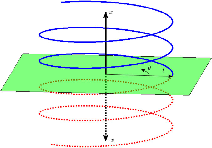
FIGURE 1. A doubly infinite helical vortex of constant pitch (p, not shown) and radius (t) extends from +∞ to −∞. The negative x−axis and vortex for negative x are shown as dashed lines. The first aim of the present work is to extend the analysis that gives the induced velocities in the green plane for any radius (r), but θ = 0 only to any (r, θ). θ = 0 is defined by the intersection of the vortex and the green plane. The induced velocities, (u, v, w), are in the (x, r, θ) directions.

The next section describes the KH equations and their two-term approximations for the velocities along the LLs and the new extension to the whole rotor plane. Then, the third-order approximations are derived and compared to those due to Okulov (2004) and Okulov and Sørensen (2020), which they called “remainders.” The testing of the accuracy of the approximations is described in Section 3; the remainders are generally more accurate than the third-order corrections. As mentioned above, a major complication is that the KH equations apply to a doubly infinite helical vortex, whereas the velocities at x = 0 are needed for the trailing blue vortex in Figure 1. When θ = 0, the singly infinite induced velocities are one-half the doubly infinite ones; it is shown at the start of Section 4 that the doubly infinite results for non-zero θ give the sum of the induced velocities at ±θ for a trailing vortex, and a further relation between these velocities is needed. Section 4 continues by using the Biot–Savart law to derive an approximate further relation for the difference in the velocities at ±θ. Section 5 describes numerical tests of the singly infinite equations. Section 6 discusses the results, shows how the analysis can be extended to coned rotors, and contains the conclusions. Appendix A describes the derivation of the sums needed for the θ − dependent approximations, and Appendix B shows the three terms in the approximation integration to zero over the region of planar symmetry as a check on the consistency of the derivation. Appendix C presents the analytic remainders added to the numerical integral of the Biot–Savart law for the singly infinite helices.

2 The equations for the velocities induced by doubly infinite helices

2.1 The exact equations

Cylindrical polar coordinates are used: (x, r, θ), where x is in the axial or streamwise direction, r is the radius, and θ is the circumferential angle. The respective velocity components are (u, v, w). A doubly infinite helical vortex of constant pitch p, defined by dx/dθ = p for any point on the vortex, passes through (0, t, 0), as shown in Figure 1. The vortex radius remains t throughout the wake. u at any point (0, r, θ) along straight and radial LLs is given by the KH equations, Kawada (1936), Kawada (1939), and Hardin (1982), as described, for example, in Wood et al. (2021):

$u\left(r,\theta \right)=\bar{u}\left(r\right)+u^{\prime }\left(r,\theta \right)=\left\{\begin{array}{cc}\frac{\mathrm{\Gamma }}{2\pi p}-\frac{\mathrm{\Gamma }t}{\pi p^2}{S}_1\hfill & \text{if}r<t,\hfill \\ \hfill \\ -\frac{\mathrm{\Gamma }t}{\pi p^2}{S}_3\hfill & \text{if}r>t.\hfill \end{array}\right.(1)$

Here, Γ is the vortex strength, and the overline indicates a circumferentially averaged value. Similarly, the circumferential velocity, w, is given by

$w\left(r,\theta \right)=\bar{w}\left(r\right)+w^{\prime }\left(r,\theta \right)=\left\{\begin{array}{cc}\frac{\mathrm{\Gamma }t}{\pi pr}{S}_1\hfill & \text{if\hspace{0.17em}}r<t,\hfill \\ \hfill \\ \frac{\mathrm{\Gamma }}{2\pi r}+\frac{\mathrm{\Gamma }t}{\pi pr}{S}_3\hfill & \text{if\hspace{0.17em}}r>t.\hfill \end{array}\right.(2)$

Note that the mean velocity only appears for r < t in Eq. 1 and for r > t in (2). Thus, only the vortices above a blade element contribute to its mean axial velocity, and only those below it, to the mean circumferential velocity. Furthermore, the perturbation velocities determined by S₁ and S₃ are directly related by “helical symmetry”: pu′(r, θ) = −rw′(r, θ), which simplifies their computation. It is noted that helical symmetry also relates $\bar{u}(r,\theta )$ to $\bar{w}(r,\theta )$, but its demonstration relies on Kelvin’s theorem for the strength of the vortices trailing from the top and bottom of each blade element and is not needed here. As noted above, Eqs (1) and (2) apply to a doubly infinite vortex. The series S₁ and S₃ in the notation of Hardin (1982) are given by

$S_1={\displaystyle \sum _{m=1}^{\infty }}m{K}_m^{\prime }\left(mt/p\right)I_m\left(mr/p\right)\cos \left(m\theta \right)(3)$

and

$S_3={\displaystyle \sum _{m=1}^{\infty }}m{I}_m^{\prime }\left(mt/p\right)K_m\left(mr/p\right)\cos \left(m\theta \right).(4)$

Here, I_m(.) and K_m(.) are modified Bessel functions in standard notation. m denotes the order and the prime a derivative with respect to the argument. In practice, the derivatives are evaluated using the standard results $I_m^{\prime }(.)=(I_{m-1}(.)+I_{m+1}(.))/2$ and $K_m^{\prime }(.)=-(K_{m-1}(.)+K_{m+1}(.))/2$.

S₁ and S₃ completely determine both u and w, which are the focus of this study. The induced radial velocity, v, is generally ignored in BEMT, but this may not be justified for coned and swept rotors if the radial flow over the blade elements alters the element’s lift and drag. v may also be important for any rotor with significant expansion of the wake as u and v have the same magnitude for any swept or unswept rotor and any wake expansion (Limacher and Wood, 2021). There are two main problems in extending the present analysis to v. The first is that a significant v implies a significant variation in the vortex radius, t, for which no analytic solutions are known. Second, the series for v when t is constant, S₂ and S₄ in the notation of Hardin (1982), involve products of $I_m^{\prime }(.)$ and $K_m^{\prime }(.)$ and would need extra analysis to produce the rotor plane approximations. v is not considered further in this study. Note that the terms involving S₁ and S₃ give the perturbations from the streamtube averages. The perturbations must integrate to zero over the azimuthal region of symmetry, 2π/N, where N is the number of blades. This constraint will be used later to check the approximate equations for u′ and w′.

Clearly, Γ must be known to convert S₁ and S₃ into induced velocities. In the BEMT, Γ is the difference in the bound circulation of the elements on either side of the trailing vortex whose induced velocity is being calculated. Γ is easily determined from the element lift and drag, but this determination is outside the scope of the present work. All other parameters for the induced velocities are set by the rotor geometry, except for p. It can be calculated from the blade element thrust and torque, or equivalently, from $\bar{u}$ and $\bar{w}$ immediately behind the blades (Wood and Hammam, 2022).

Wood et al. (2021) analyzed methods to find u and w at x = θ = 0 due to a vortex also starting at x = θ = 0. This restricted the analysis to straight, radial blades. Removing this restriction is the purpose of the present analysis, which is made easier by the dependence of S₁ and S₃ on θ being separate from that on the coordinates and length parameters. Thus, each term in the Kapteyn-like series of products of Bessel functions and their derivatives in S₁ and S₃ can be summed over the N blades before summing the series in m, as explained by Wood et al. (2021). The circumferential summation is exact only if the blades are identical and equispaced, which can hold for swept and straight blades and will be assumed here. Summing over the N blades introduces what Wood et al. (2021) called “Kawada” cancellation: the original 2π azimuthal periodicity of a single trailing vortex becomes a 2π/N periodicity of N identical vortices, and this cancels a fraction of (N − 1)/N of the terms in the sums.

With Kawada cancellation, S₁ and S₃ reduce to

$S_1=N{\displaystyle \sum _{m=1}^{\infty }}mN{K}_{mN}^{\prime }\left(mNt/p\right)I_{mN}\left(mNr/p\right)\cos \left(mN\theta \right)(5)$

and

$S_3=N{\displaystyle \sum _{m=1}^{\infty }}mN{I}_{mN}^{\prime }\left(mNt/p\right)K_{mN}\left(mNr/p\right)\cos \left(mN\theta \right).(6)$

All further references to S₁ and S₃ are to these equations for N blades which, obviously, include N = 1 as a special case.

Kawada cancellation removes two-thirds of the terms if N = 3, but the exact series for the induced velocities remains numerically challenging, partly because the number of terms required for a specified accuracy increases without bound as r → t. Wood et al. (2021) described the considerable historical effort to develop accurate approximate equations. The next section describes those of Wrench (1957), which were shown by Wood et al. (2021) to be the most accurate two-term approximations.

2.2 Wrench’s approximate equations

Wrench used the asymptotic expansion of I_m(.) by Lehmer (1944) and his own, a similar expansion of K_m(.). Eq. 19 of Wrench (1957) gives the m−th term in S₁ for θ = 0, in the present notation, as

$\begin{array}{ll}\hfill & mN{K}_{mN}^{\prime }\left(mNt/p\right)I_{mN}\left(mNr/p\right)\hfill \\ \hfill & \sim -A{U}_W^m\left(1+\frac{{\left(t/p\right)}^2}{2mN{c}_t^3}\right)\exp \left(\frac{{\psi }_1\left({\left(r/p\right)}^2\right)}{mN{c}_r^3}-\frac{{\psi }_1\left({\left(t/p\right)}^2\right)}{mN{c}_t^3}\right),\hfill \end{array}(7)$

where the parentheses show only the first two terms that Wrench retained in each expansion. In (7),

$\begin{array}{ll}A\hfill & =\frac{p}{2t}\sqrt{\frac{c_t}{c_r}},\text{\hspace{0.17em}where\hspace{0.17em}}{c}_t=\sqrt{1+{\left(t/p\right)}^2},c_r=\sqrt{1+{\left(r/p\right)}^2},\text{\hspace{0.17em}and\hspace{0.17em}}\hfill \\ U_W\hfill & ={\left[\frac{t\left(c_r-1\right)}{r\left(c_t-1\right)}\exp \left(c_r-c_t\right)\right]}^N.\hfill \end{array}(8)$

The function ψ₁ is defined as

${\psi }_1\left(z^2\right)=\left(3z^2-2\right)/24(9)$

for any z, from Wrench’s Eq. 11. For readers interested in the details of the derivation of the induced velocities, Table 1 relates the variables used in the present analysis to Wrench’s equations.

TABLE 1

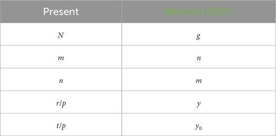
TABLE 1. Correspondence of the present symbols to Wrench (1957).

Wrench expanded the exponential term in (7) to the leading order in ψ₁ to yield

$\begin{array}{ll}\hfill & mN{K}_{mN}^{\prime }\left(mNt/p\right)I_{mN}\left(mNr/p\right)\hfill \\ \hfill & \sim -A{U}_W^m\left(1+\frac{{\left(t/p\right)}^2}{2mN{c}_t^3}\right)\left(1+\frac{3{\left(r/p\right)}^2-2}{24mN{c}_r^3}-\frac{3{\left(t/p\right)}^2-2}{24mN{c}_t^3}\right)\hfill \\ \hfill & \sim -A{U}_W^m\left(1+\frac{B}{mN}\right),\hfill \end{array}(10)$

where

$B=\frac{1}{24}\left[\frac{9{\left(t/p\right)}^2+2}{c_t^3}+\frac{3{\left(r/p\right)}^2-2}{c_r^3}\right].(11)$

Note that A and B are independent of m and, for future purposes, θ. The approximation for each term in S₃ was developed analogously from Eq. 20 of Wrench (1957):

$\begin{array}{ll}\hfill & mN{I}_{mN}^{\prime }\left(mNt/p\right)K_{mN}\left(mNr/p\right)\hfill \\ \hfill & \sim A{U}_W^{-m}\left(1-\frac{{\left(t/p\right)}^2}{2mN{c}_t^3}\right)\exp \left(\frac{{\psi }_1\left({\left(t/p\right)}^2\right)}{mN{c}_t^3}-\frac{{\psi }_1\left({\left(r/p\right)}^2\right)}{mN{c}_r^3}\right)\hfill \\ \hfill & \sim A{U}_W^{-m}\left(1-\frac{{\left(t/p\right)}^2}{2mN{c}_t^3}\right)\left(1+\frac{3{\left(t/p\right)}^2-2}{24mN{c}_t^3}-\frac{3{\left(r/p\right)}^2-2}{24mN{c}_r^3}\right)\hfill \\ \hfill & \sim A{U}_W^{-m}\left(1-\frac{B}{mN}\right).\hfill \end{array}(12)$

For both S₁, with U_W < 1, and S₃, with U_W > 1, the summation over 1 ≤ m < ∞ is easy for the A − term as it is a geometric series. Added to the sum of the second term derived in Appendix A, Wrench’s approximations become

$S_{1,W}=-A\left[\frac{N{U}_W}{1-U_W}+B\log \left(1+\frac{U_W}{1-U_W}\right)\right](13)$

for r < t and

$S_{3,W}=A\left[\frac{N}{U_W-1}-B\log \left(1+\frac{1}{U_W-1}\right)\right](14)$

for r > t, which are Eqs 15, 16 of Wood et al. (2021). It is clear from Eqs 13, 14 that S_1,W and S_3,W become singular as r → t and U_w → 1. This is the situation mentioned above, which causes the unbounded increase in the number of terms in the Kapteyn series that must be summed to achieve a specified accuracy. A major advantage of the approximate solutions is that they remain accurate for any U_W ≠ 1 (Wood et al., 2021).

Including θ in the approximations is straightforward. The second line of Eq. 10 becomes

$\begin{array}{ll}\hfill & mN{K}_{mN}^{\prime }\left(mNt/p\right)I_{mN}\left(mNr/p\right)\cos \left(mN\theta \right)\hfill \\ \hfill & \sim -A{U}_W^m\left(1+\frac{B}{mN}\right)\cos \left(mN\theta \right),\hfill \end{array}(15)$

and the same factor of cos(mNθ) multiplies the right sides of (12). The results in Appendix A allow the generalization of Eqs 13, 14 to be

$\begin{array}{ll}\hfill S_{1,W}=& -A\left[N\frac{U_W\left(\cos \left(N\theta \right)-U_W\right)}{1+U_W^2-2U_W\cos \left(N\theta \right)}\right.\hfill \\ \hfill & \left.-\frac{B}{2}\log \left(1+U_W^2-2U_W\cos \left(N\theta \right)\right)\right]\hfill \end{array}(16)$

for r < t and

$\begin{array}{ll}\hfill S_{3,W}=& A\left[N\frac{U_W\cos \left(N\theta \right)-1}{1+U_W^2-2U_W\cos \left(N\theta \right)}\right.\hfill \\ \hfill & \left.+\frac{B}{2}\log \left(\frac{1+U_W^2-2U_W\cos \left(N\theta \right)}{U_W^2}\right)\right]\hfill \end{array}(17)$

for r > t. It will be shown in Section 3 that the second term, which will be called the “B − term” despite it containing A, is typically small compared to the A − term. Both terms become singular as r → t and U_W → 1, but only when θ = 0. This singularity is associated with the complex nature of the flow in the immediate vicinity of the vortex, e.g., Boersma and Wood (1999) and Okulov and Sørensen (2020), and does not appear to detract from the usefulness of the equations for computing the induced velocities for LL analysis.

2.3 Higher-order terms in Wrench’s expansion

The next term in Wrench’s expansion has not been derived previously in the open literature. It is now given for S₁, and the very similar result for S₃ will be quoted. Extending (10) gives

$\begin{array}{ll}\hfill & mN{K}_{mN}^{\prime }\left(mNt/p\right)I_{mN}\left(mNr/p\right)\hfill \\ \hfill & \sim -A{U}_W^m\left(1+\frac{{\left(t/p\right)}^2}{2mN{c}_t^3}+\frac{{\left(t/p\right)}^2\left(4-{\left(t/p\right)}^2\right)}{8{\left(mN{c}_t^3\right)}^2}\right)\hfill \\ \hfill & \exp \left[{\displaystyle \sum _{n=1}^2}\left(\frac{{\psi }_n\left({\left(r/p\right)}^2\right)}{{\left(mN{c}_r^3\right)}^n}+{\left(-1\right)}^n\frac{{\psi }_n\left({\left(t/p\right)}^2\right)}{{\left(mN{c}_t^3\right)}^n}\right)\right]\hfill \\ \hfill & \sim -A{U}_W^m\left(1+\frac{B}{mN}+\frac{C_W}{m^2{N}^2}\right).\hfill \end{array}(18)$

Since

${\psi }_2\left(z^2\right)=z^2\left(z^2-4\right)/16(19)$

for any z, from Eq. 11 of Wrench (1957), C_W is obtained as

$\begin{array}{ll}\hfill C_W& =\frac{1}{16}\left[\frac{1}{c_r^6}\left(\frac{9{\left(r/p\right)}^4}{8}-\frac{25{\left(r/p\right)}^2}{6}+\frac{1}{18}\right)\right.\hfill \\ \hfill & +\frac{1}{c_r^3{c}_t^3}\left(\frac{3{\left(r/p\right)}^2{\left(t/p\right)}^2}{4}+\frac{{\left(r/p\right)}^2}{6}-\frac{{\left(t/p\right)}^2}{2}-\frac{1}{9}\right)\hfill \\ \hfill & -\left.\frac{1}{c_t^6}\left(\frac{15{\left(t/p\right)}^4}{8}-\frac{9{\left(t/p\right)}^2}{2}-\frac{1}{18}\right)\right].\hfill \end{array}(20)$

Using the results from Appendix A, S_1,W becomes

$\begin{array}{ll}\hfill S_{1,W}& =-A\left[N\frac{U_W\left(\cos \left(N\theta \right)-U_W\right)}{1+U_W^2-2U_W\cos \left(N\theta \right)}\right.\hfill \\ \hfill & -\frac{B}{2}\log \left(1+U_W^2-2U_W\cos \left(N\theta \right)\right)\hfill \\ \hfill & +\left.\frac{C_W}{2N}\left\{{\text{Li}}_2\left(U_W{\text{e}}^{iN\theta }\right)+{\text{Li}}_2\left(U_W{\text{e}}^{-iN\theta }\right)\right\}\right]\hfill \end{array}(21)$

for r < t, and the extended S_3,W for r > t is

$\begin{array}{ll}\hfill S_{3,W}& =-A\left[N\frac{U_W\cos \left(N\theta \right)-1}{1+U_W^2-2U_W\cos \left(N\theta \right)}\right.\hfill \\ \hfill & +\frac{B}{2}\log \left(\frac{1+U_W^2-2U_W\cos \left(N\theta \right)}{U_W^2}\right)\hfill \\ \hfill & +\left.\frac{C_W}{2N}\left\{{\text{Li}}_2\left({\text{e}}^{iN\theta }/U_W\right)+{\text{Li}}_2\left({\text{e}}^{-iN\theta }/U_W\right)\right\}\right].\hfill \end{array}(22)$

Li₂(.) in these equations is the dilogarithm function, described in chapter 25 of DLMF (2023). As mentioned above, S₁ and S₃ give the perturbations from the circumferential average velocities in the rotor plane. Because A, B, and C are not related, the A −, B −, and C − terms must individually integrate to zero over [0, 2π/N]. Appendix B shows this to be the case for all three, which provides a check on the derivation of the θ−dependent terms.

2.4 Higher-order terms due to Okulov

Okulov (2004) and Okulov and Sørensen (2020) used an alternative strategy to the asymptotic expansion of the Bessel functions in S₁ and S₃. They separated “the key terms from the series” and developed remainders to improve the accuracy. Wood et al. (2021) showed the key terms are identical to Wrench’s two-term approximations in Eqs 13, 14 for θ = 0, and, by implication, to (16) and (17) for non-zero θ. Following the recommendation of Okulov and Sørensen (2020) to use only the first term in their Eq. (A6a), the alternative C − term, C_1,O, for S₁ in the present notation is

$C_{1,O}=\left(K_1^{\prime }\left(t/p\right)I_1\left(r/p\right)+A{U}_O\left(1+B\right)\right)\cos \left(\theta \right),(23)$

where U_O = U_W for N = 1. Using (15), the leading term in C_1,O is

$C_{1,O}\sim -A{U}_{O}C\cos \left(\theta \right),(24)$

and for S_3,O is

$C_{3,O}\sim AC\cos \left(\theta \right)/U_O.(25)$

In the numerical experiments described in Section 3, the approximations, S_1,O and S_3,O, are given in Eqs (21) and (22), respectively, with the C − term replaced by either (24) or (25).

3 Numerical tests of the approximate doubly infinite equations

Wood et al. (2021) documented the range of pitch values for a number of simulations and experiments on wind and hydrokinetic turbines and propellers, which led them to choose representative values of p = 0.1, 1 and N = 4 for their numerical tests to determine the accuracy of the approximate equations for θ = 0. The accuracy depends on N, but the dependence on p is stronger; decreasing p, which corresponds to increasing the tip speed ratio for turbines, increases the accuracy. Because of the close similarity between S₁ and S₃, only the former is considered here for N = 3. S₁ was calculated directly from Eq. 5 by summing to a maximum value of m = m_max, chosen to give an accuracy of 10^–8 using Eq. 18 of Wood et al. (2021), which assumes θ = 0. Since the Kapteyn series will converge more rapidly for θ ≠ 0, using an upper limit of m_max ∀ θ should be safe. S_1,A is the A − term in the approximation, that is, the first term in (21), and S_1,W includes all three terms.

The results shown in Figure 2 correspond to a tip speed ratio of approximately 7, and t = 1 and r = 0.99 represent the tip vortex and the center of the blade element at the tip, respectively, when the number of elements per blade is around 50. Since S₁ and S₃ are even in θ, 200 equispaced points over the positive region of symmetry, θ = [0, π], were computed, but only every fifth point is plotted in the main figure. The inset amplifies the region near θ = 0 for all points in that region. For these conditions, m_max = 59, indicating the considerable computational burden of summing the exact equations. Wrench’s approximation is very accurate; the r.m.s difference between S₁ and S_1,W over the 200 points calculated for 0 ≤ θ ≤ π/N was almost within the tolerance of calculating S₁. Using the A − term only gives reasonable accuracy at p = 0.1. For θ = 0, S₁ = −0.43172, S_1,A = −0.42838, and S_1,W = −0.43172; so using the first term only in the approximation gives a modest error of less than 1%.

FIGURE 2

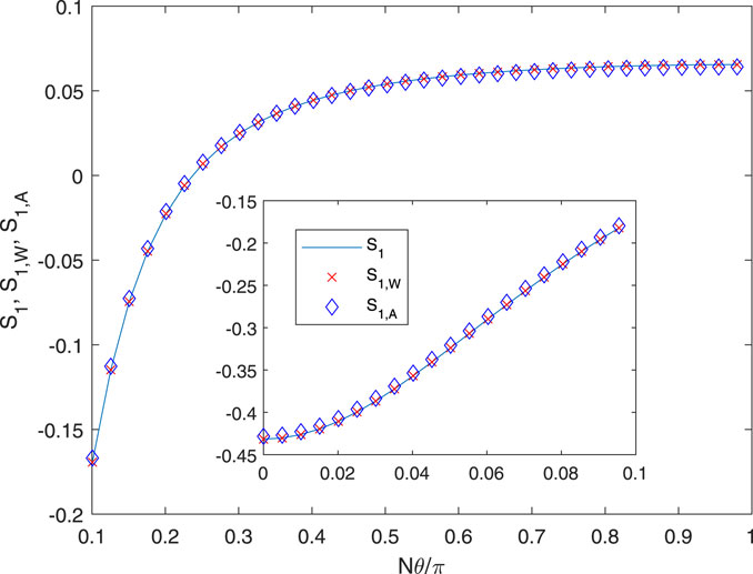
FIGURE 2. S₁, S_1,W, and S_1,A for p = 0.1, r = 0.99, and t =1.

It is inferred from these results that the C − term or Okulov’s alternative is not significant at this p. Their behavior is shown in Figure 3. Okulov’s third term, Eq. 24, is more accurate than C_W from (21), but both could be used to determine the accuracy of using only two terms, i.e., Eqs 16, 17. Increasing p to p = 1 increases the time required for the evaluation of the exact solution. For the same N, t, and r, m_max becomes 519, and an accurate summation was not possible. r was decreased to 0.98, for which m_max = 250. The results are shown in Figures 4, 5. At θ = 0, S₁, S_1,W, and S_1,A were 1.7152, 1.7154, and 1.6933, respectively, all multiplied by 10⁴. The accuracy of the approximations is slightly worse than that at p = 0.1, and Figure 5 shows that the two versions of the C − term have become nearly equal. In particular, it is noted that the A − term is a significantly poorer approximation to the exact solution at its higher p.

FIGURE 3

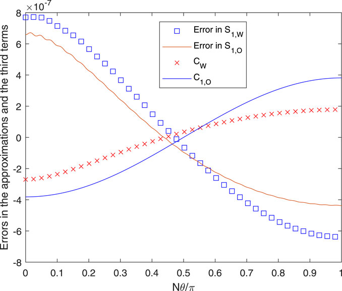
FIGURE 3. Errors and third terms for the conditions in Figure 2.

FIGURE 4

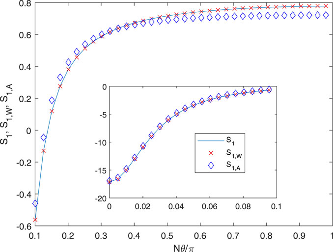
FIGURE 4. S₁, S_1,W, and S_1,A for p =0.1, r =0.1, and t = 1.

FIGURE 5

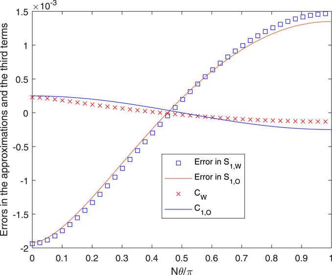
FIGURE 5. Errors and third terms for the conditions in Figure 4.

Other combinations of N, p, t, and r were investigated but not presented as the results shown are typical. The extension of Wrench’s approximations for θ = 0 to any θ was found to be accurate for a representative range of the parameters, and the accuracy can be improved and/or assessed by the C − term or Okulov’s alternative.

4 The velocities induced by a singly infinite vortex over the rotor plane

All the equations derived and tested so far apply to a doubly infinite helical vortex. They give twice the velocities induced by a singly infinite (trailing) vortex only when θ = 0. For non-zero θ, it will be shown below that the doubly infinite equations give u(r, θ) + u(r, − θ) and w(r, θ) + w(r, − θ) for a singly infinite vortex, and a further relation between the velocities is needed. Approximate relations for u(r, θ) − u(r, − θ) and w(r, θ) − w(r, − θ) can be derived from the Biot–Savart (BS) law for a line vortex.

Since the BS law provides a different method for determining the induced velocities, its relation to the KH equations, (1)–(4), is now briefly considered. The KH equations were derived from the velocity potential of a flow containing a doubly infinite helical vortex. The relationship with the BS law was analyzed by Morgan and Wrench (1965) and, more accessibly, by Boersma and Yakubovich (1998), whose Eq. 1 establishes the BS law as the “integral representation” of the series involving S₁ and S₃; see also Eq. (2.6) of Boersma and Wood (1999).

A straightforward application of the BS law gives

$\left(u\left(r,\theta \right),w\left(r,\theta \right)\right)=\frac{\mathrm{\Gamma }}{4\pi }\left(I_{u,BS},I_{w,BS}\right)=\frac{\mathrm{\Gamma }}{4\pi }{\int }_0^{\infty }\frac{\left(i_u\left(r,\theta \right),i_w\left(r,\theta \right)\right)}{d^3}d\beta ,(26)$

where Γ is the vortex strength and β is the angle which is positive in the direction of positive θ. I_u and I_w, called the “influence functions,” depend only on the geometry of the vortex. The limits indicate a singly infinite vortex so that β = [0, ∞] for both θ and −θ. The integrands contain

$\begin{array}{ll}\hfill i_u\left(r,\theta \right)& =t^2-rt\cos \left(\beta -\theta \right)\text{and}\hfill \\ \hfill i_w\left(r,\theta \right)& =p\left(r-t\cos \left(\beta -\theta \right)-t\beta \sin \left(\beta -\theta \right)\right),\hfill \end{array}(27)$

and the distance d is given by

$d^2\left(r,\theta \right)=r^2+t^2-2rt\cos \left(\beta -\theta \right)+p^2{\beta }^2.(28)$

The relationship between the doubly and singly infinite velocities can be seen from

$\begin{array}{ll}\hfill {\int }_{-\infty }^{\infty }\frac{i_u\left(r,\theta \right)}{d^3\left(r,\theta \right)}d\beta & ={\int }_0^{\infty }\frac{i_u\left(r,\theta \right)}{d^3\left(r,\theta \right)}d\beta +{\int }_{-\infty }^0\frac{i_u\left(r,\theta \right)}{d^3\left(r,\theta \right)}d\beta \hfill \\ \hfill & ={\int }_0^{\infty }\frac{i_u\left(r,\theta \right)}{d^3\left(r,\theta \right)}d\beta +{\int }_0^{\infty }\frac{i_u\left(r,-\theta \right)}{d^3\left(r,-\theta \right)}d\beta \hfill \\ \hfill & =I_{u,BS}\left(r,\theta \right)+I_{u,BS}\left(r,-\theta \right).\hfill \end{array}(29)$

It follows from (26) that

$\int \frac{p{i}_u\left(r,\theta \right)+r{i}_w\left(r,\theta \right)}{d^3\left(r,\theta \right)}d\beta =\frac{p\beta }{\sqrt{t^2+r^2-2rt\cos \left(\theta -\beta \right)+p^2{\beta }^2}}.(30)$

By this extended version of helical symmetry, w(r, θ) can be obtained immediately from u(r, θ), so only the latter will be analyzed. Despite (30), the integrals for a helical vortex do not have closed-form solutions. Thus, the following approximation is made for the difference in the influence functions:

$\mathrm{\Delta }{I}_u=I_u\left(r,\theta \right)-I_u\left(r,-\theta \right)\approx \mathrm{\Delta }{I}_{u,1}={\int }_0^{2\theta }\frac{i_u\left(r,\theta \right)}{{\left(r^2+t^2-2rt\cos \left(\beta -\theta \right)+z^2\right)}^{3/2}}d\beta ,(31)$

where z = pθ. In words, the difference in the velocities is approximately that induced by a sector of a vortex ring of radius t located a distance pθ behind the control point. The approximation is sketched and further explained in Figure 6. In terms of β, measured from the intersection of the blue vortex and the green plane, the sector starts at (t, 0) and ends at (t, 2θ). The integral in (31) has an analytic form that must be modified to give the correct asymptotic behavior as r ↓ 0 for any t. In that limit, the integrand in (26) becomes independent of θ, and so ΔI_u → 0. The result obtained using Mathematica is

$\begin{array}{ll}\hfill \mathrm{\Delta }{I}_{u,1}& =\frac{2}{\sqrt{{\left(r-t\right)}^2+z^2}}\left[\frac{r^2-t^2+z^2}{{\left(r+t\right)}^2+z^2}E\left(\frac{\theta }{2},\frac{-4rt}{{\left(r-t\right)}^2+z^2}\right)\right.\hfill \\ \hfill & \left.-F\left(\frac{\theta }{2},\frac{-4rt}{{\left(r-t\right)}^2+z^2}\right)\right]\hfill \\ \hfill & +\frac{4rt\left(r^2-t^2+z^2\right)\sin \left(\theta \right)}{\left(r^4+2r^2\left(z^2-t^2\right)+{\left(t^2+z^2\right)}^2\right)\sqrt{r^2+t^2+z^2-2rt\cos \left(\theta \right)}}\hfill \\ \hfill & +\frac{2t^2\theta }{{\left(t^2+z^2\right)}^{3/2}},\hfill \end{array}(32)$

where E(. , .) and F(. , .) are the incomplete elliptic integrals described in chapter 19 of DLMF (2023). The extra subscript was added to ΔI_u to denote the use of the full form of the integrals. Two more approximations with different additional subscripts are described below.

FIGURE 6

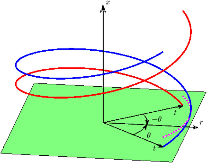
FIGURE 6. Difference in velocities induced by the blue and red singly infinite vortices anywhere along radius r is approximately the velocity induced by the vortex sector shown in dashed magenta. The sector of radius t spans [−θ, θ] and is parallel to the green plane and distance pθabove it.

As for the doubly infinite results in Section 3, the tests on the accuracy of the approximations are restricted to r < t. A single vortex (N = 1) only will be considered, but some comments on the important cases of N > 1 are made below. The sum of the influence functions is

$\mathrm{\Sigma }{I}_u=I_u\left(r,\theta \right)+I_u\left(r,-\theta \right)\approx \mathrm{\Sigma }{I}_{u,W}=\frac{t}{p^2}{S}_{1,W}(33)$

when the C − terms are ignored on the grounds that they are likely to be comparable to, or smaller than, the errors in using (32) for most turbine applications. The extra subscript in I_u,W indicates that it was determined from Eq. 16. For comparison, the “exact” values of I_u,BS(θ) and I_u,BS(−θ) were determined by the numerical evaluation of the Biot–Savart integral for I_u in (26) using MATLAB's integral function with the default error settings, over β = [0, β_max], from which ΔI_u,BS and ΣI_u,BS follow. To the latter was added an analytic remainder approximating the integrals over [β_max, ∞], as described in Appendix C. β_max = 1000π was used for all results presented here. By varying β_max, this value was found to result in 6-figure accuracy for the results presented in the next section.

ΣI_u,BS provides a check on the accuracy of ΣI_u,W from (33). ΔI_u,BS will be used to show the errors in ΔI_u,1 from Eq. 32, and further approximations using the simplification of the incomplete elliptic integrals described below. It is emphasized that the KH equations were found to give nearly identical results to those from the BS integration, but they are not considered further as they do not lead to an equation for ΔI_u.

Eq 33 is valid for all N, and it is unlikely that further simplification is possible. Eq. 32, however, has to be summed over N blades spaced 2π/N apart in a BEMT code, which raises three important considerations. First, the incomplete elliptic integrals are only partially periodic, as demonstrated by the small-modulus approximations of formulas (62:9:5) and (62:9:6) of Oldham et al. (2009):

$F\left(\frac{\theta }{2},m\right)\sim \frac{\theta }{2}+\frac{m}{4}\left(\theta -\frac{1}{2}\sin \left(\theta \right)\right)\mathrm{a}\mathrm{n}\mathrm{d}E\left(\frac{\theta }{2},m\right)\sim \frac{\theta }{2}-\frac{m}{4}\left(\theta -\frac{1}{2}\sin \left(\theta \right)\right).(34)$

Thus, summation over N blades will not allow simple Kawada cancellation. Second, the integrals are computationally expensive to evaluate, so the accuracy of using (34) was tested. Surprisingly, the most accurate overall results came from ignoring the terms in m, leaving only θ/2 for both F and E, which is very easy for summing. Using (34), without any further modification to (32), leads to the second approximation to ΔI_u:

$\begin{array}{ll}\hfill \mathrm{\Delta }{I}_{u,2}=& 2t\theta \left[\frac{t}{{\left(t^2+z^2\right)}^{3/2}}-\frac{r+t}{\left({\left(r+t\right)}^2+z^2\right)\sqrt{{\left(r-t\right)}^2+z^2}}\right]\hfill \\ \hfill & +\frac{4rt\left(r^2-t^2+z^2\right)\sin \left(\theta \right)}{\left(r^4+2r^2\left(z^2-t^2\right)+{\left(t^2+z^2\right)}^2\right)\sqrt{r^2+t^2+z^2-2rt\cos \left(\theta \right)}},\hfill \end{array}(35)$

which will be tested for accuracy along with ΔI_u,1 from (32).

The third consideration is that the trigonometric term will simplify by Kawada cancellation when summed over N blades, but the presence of cos(θ) in the denominator makes the result more complicated than that for the KH equations. Summing over N blades is equivalent to using the trapezoidal rule to approximate the integral of the periodic function:

$\begin{array}{ll}\hfill & {\int }_{\theta }^{\theta +2\pi }\frac{\sin \left(\beta \right)}{\sqrt{r^2+t^2+z^2-2rt\cos \left(\beta \right)}}d\beta \hfill \\ \hfill & =\frac{1}{\sqrt{\left.r^2+t^2+z^2\right)}}{\int }_{\theta }^{\theta +2\pi }\frac{\sin \left(\beta \right)}{\sqrt{1-a\cos \left(\beta \right)}}d\beta =0,\hfill \end{array}(36)$

where a = 2rt/(r² + t² + z²) satisfies 0 < a < 1 for a BEMT code. Note that the integral is independent of θ, but generally, the trapezoidal approximation is not, even though Kawada cancellation always applies. In the limit of a = 0, however, the sum over N is zero for any θ. Thus, the sum of the trigonometric term, which is common to ΔI_u,1 and ΔI_u,2, tends to zero as r ↓ 0 for N > 1. When a = 1, the integrand reduces to $\sqrt{2}\cos (\beta /2)$ for β < 2π and $-\sqrt{2}\cos (\beta /2)$ for β > 2π, again giving a closed-form sum. The general form of the sum is complicated and does not converge monotonically to zero at large N, probably because the complex variable form of the second integrand in (36) is not analytic when a = 1 (Trefethen and Weideman, 2014). When a < 1, the integrand is analytic, and the sums for large N are consistent with the exponential convergence of the trapezoidal rule for analytic functions that are periodic (Trefethen and Weideman, 2014). Nevertheless, the sum for small N when a = 1 appears to allow a simple approximation for a < 1 and the small values of N in a BEMT code:

$\begin{array}{ll}\hfill {\displaystyle \sum _{i=0}^{N-1}}\frac{\sin \left(\theta +\frac{2\pi i}{N}\right)}{\sqrt{1-\cos \left(\theta +\frac{2\pi i}{N}\right)}}& =\sqrt{2}{\displaystyle \sum _{i=0}^{N-1}}\cos \left(\frac{\theta }{2}+\frac{\pi i}{N}\right)\hfill \\ \hfill & =\sqrt{2}\left[\cos \left(\frac{\theta }{2}\right)-\cot \left(\frac{\pi }{2N}\right)\sin \left(\frac{\theta }{2}\right)\right],\hfill \end{array}(37)$

provided Nθ ≤ 2π. This suggests approximating the sum for any a as

${\displaystyle \sum _{i=0}^{N-1}}\frac{\sin \left(\theta +\frac{2\pi i}{N}\right)}{\sqrt{1-a\cos \left(\theta +\frac{2\pi i}{N}\right)}}\approx \frac{\sin \left(\theta \right)}{\sqrt{1-a\cos \left(\theta \right)}}-\sqrt{2}\cot \left(\frac{\pi }{2N}\right)\sin \left(\frac{\theta }{2}\right),(38)$

which is exact for N = 1 as cot(π/2) = 0 and is accurate for other values of N < 10 approximately over a wide range of θ. Eq 37 shows that the sum becomes zero when N = π/θ, which is large for small θ. Thus, the sum of the non-analytic function when a = 1 is algebraic rather than N times the exponential convergence of the trapezoidal rule when a < 1 and N is sufficiently large.

The convergence of the sum in (38) for a < 1 inferred from that of the trapezoidal rule shows that there are no sweep effects on the induced velocities for an actuator disc that is approached as N → ∞, that is, much larger values than considered in the previous paragraph. Periodicity also requires u(π) = u(−π), that is, u(θ) → u(−θ) as θ → π. This requirement is not satisfied by either (32) or (35), but this error is unlikely to be significant for moderate sweep and coning. As shown at the end of the next section, the error can be easily corrected.

5 Numerical tests of the singly infinite equations

Figure 7 plots the influence functions over θ = [0, π] for the conditions of Figure 2, except that now N = 1, and Figure 8 shows the various ΔI_u and ΣI_u. As expected from the previous results, Wrench’s approximation for ΣI_u is very accurate at all θ. Both approximations for I_u(θ) are accurate at small θ when I_u(θ) is large in magnitude. Small θ is likely to occur frequently when the control point, r, is close to the vortex at t. There is, however, a very large difference between I_u(θ) and I_u(−θ), which remains close to zero for all θ. Only the exact influence functions asymptote to equality as θ → π, but the effect of the error in the others is likely to be small. The error is due almost entirely to the error at large θ in ΔI_u,1 and ΔI_u,2.

FIGURE 7

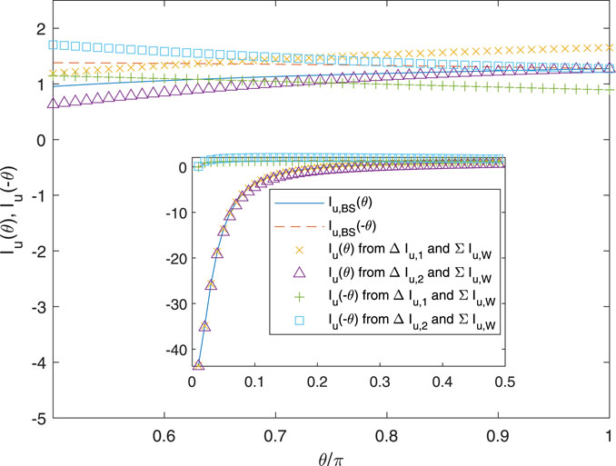
FIGURE 7. Influence functions for u(θ) and u(−θ) for N = 1, r = 0.99, t = 1.0, and p = 0.1.

FIGURE 8

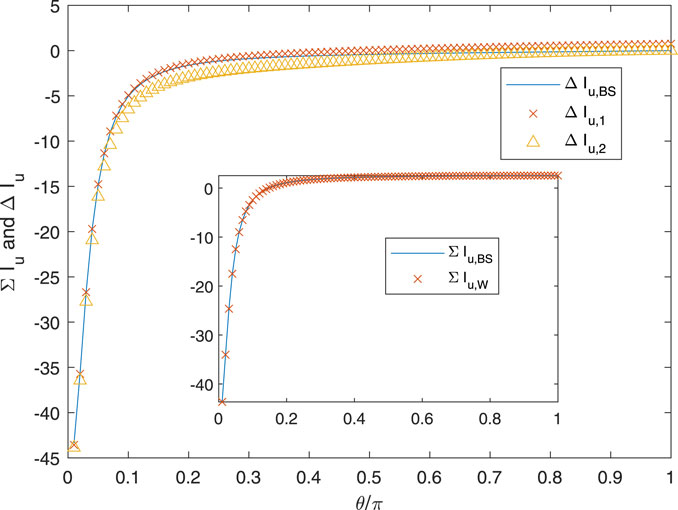
FIGURE 8. ΣI_u and ΔI_u for N = 1, r =0.99, t = 1.0, and p = 0.1.

In Figure 9 for I_u and Figure 10 for ΔI_u and ΣI_u, r has been reduced to 0.1, which places it in the hub region where θ for t = 1 is likely to be larger than for r = 0.99 in a BEMT implementation. Now, I_u(θ) is nearly equal and opposite to I_u(−θ), and the typical magnitude has decreased substantially. Both approximations for I_u differ from the exact solution at θ = π, but the error may not be significant.

FIGURE 9

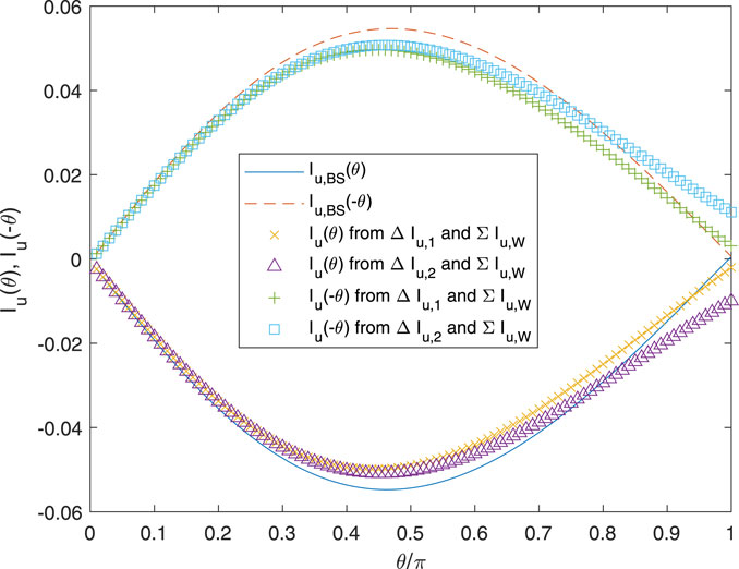
FIGURE 9. Influence functions for u(θ) and u(−θ) for N = 1, r = 0.10, t = 1.0, and p =0.1.

FIGURE 10

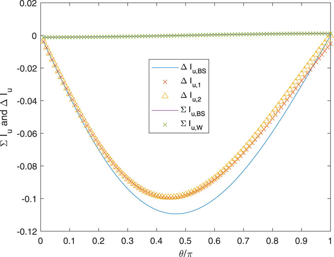
FIGURE 10. ΣI_u and ΔI_u for N = 1, r =0.10, t = 1.0, and p = 0.1.

It is possible that the errors in ΔI_u are related to placing the vortex sector at the arbitrary location of pθ behind the control point. Changes to the position of the sector were investigated, but no overall improvement in accuracy was found, so all the present results were obtained using z = pθ.

A simple way to restore the periodicity to I_u is to replace θ with sin(θ) in Eq. 35. This gives the third approximation:

$\begin{array}{ll}\hfill \mathrm{\Delta }{I}_{u,3}=& 2t\sin \left(\theta \right)\left[\frac{t}{{\left(t^2+z^2\right)}^{3/2}}-\frac{r+t}{\left({\left(r+t\right)}^2+z^2\right)\sqrt{{\left(r-t\right)}^2+z^2}}\right.\hfill \\ \hfill & +\left.\frac{2r\left(r^2-t^2+z^2\right)}{\left(r^4+2r^2\left(z^2-t^2\right)+{\left(t^2+z^2\right)}^2\right)\sqrt{r^2+t^2+z^2-2rt\cos \left(\theta \right)}}\right].\hfill \end{array}(39)$

This approximation is not shown in Figures 7–9 to ensure their clarity. Figures 11, 12 plot the accuracy of I_u,i for i = 1, 2, 3 for t = 1.0, p = 0.1, and r = 0.99 and 0.1, respectively. The “error” is I_u,BS − I_u,i, where ΣI_u,W is used for all i. Overall, the third approximation is better than the second and is sometimes better than the first. As expected from ΣI_u,W being substantially more accurate than ΔI_u,i for any i, the errors in I_u,i(θ) and I_u,i(−θ) are equal in magnitude and opposite in sign.

FIGURE 11

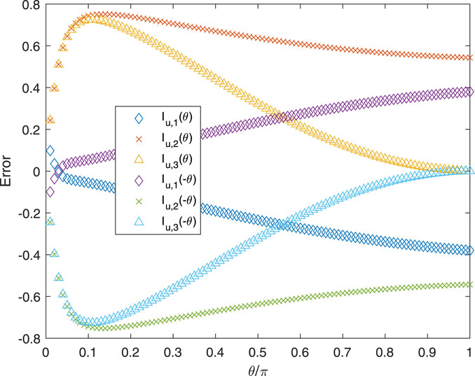
FIGURE 11. Errors in the three approximations for I_u for N = 1, r = 0.99, t = 1.0, and p = 0.1.

FIGURE 12

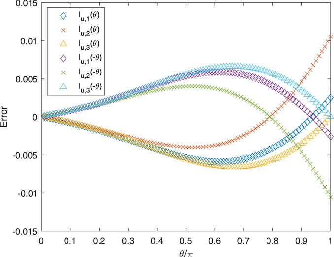
FIGURE 12. Errors in the three approximations for I_u for N = 1, r = 0.1, t =1.0, and p = 0.1.

6 Discussion and conclusion

The main aim of this study was to extend the approximate methods for computing the induced velocities along straight, radial blades of horizontal-axis turbines and propellers, as described by Wood et al. (2021), to the whole rotor plane for blades that are swept. This extension also provides accurate approximations of the induced velocities for a swept or nonswept rotor anywhere in the plane of rotation. The basis for the analysis is the approximations derived by Wrench (1957) for the exact Kawada–Hardin (KH) equations for the velocity field of a doubly infinite vortex of constant pitch and radius. These equations involve infinite sums of products of Bessel functions and their derivatives, which cannot be evaluated quickly and accurately in many cases. The extension of the approximate equations is straightforward because the generalized sums described in Appendix A are not significantly more complicated than those needed to determine the velocities along straight and radial blades. Furthermore, blade element/momentum theory (BEMT) requires the induced velocities in the axial and circumferential directions. For all parts of the present analysis, there is a close connection between them, so only the axial velocity was considered in detail.

Comparison to the exact solutions showed the extended approximate equations are accurate. For some operating conditions, sufficient accuracy may be obtained using the first or A − term. Two different third-order or C − terms were used. The first extended the expansion of the Bessel functions by Wrench (1957) to the third order, and the second was the leading-order approximation to the alternative treatment of Okulov (2004) and Okulov and Sørensen (2020). The two expressions give similar results, but Okulov’s expression is more accurate.

The application of the analysis in a blade element/momentum theory (BEMT) code must consider the differences between the doubly infinite results from the KH equations and the singly infinite vortices trailing from the junctions of the blade elements. For an angle θ between the origin of the trailing vortex and the control point, the KH equations give the sum of the velocities at ±θ. An additional, approximate equation for the difference in the velocities was derived from the Biot–Savart law. This equation contains incomplete elliptic integrals, which are computationally expensive to evaluate, so the first term in their low-modulus expansion was tested. This term was found to lead to accurate values of the induced velocity for small values of θ, but the accuracy reduced as θ approached π, which may well be applicable for the velocity induced in the hub region by the tip vortex.

The most interesting results from the previous section are those in Figures 7, 8 for small |θ|, where u(θ) is much larger in magnitude than u(−θ). This suggests that the induced velocities when the blade is swept forward, whereby the tip is “ahead” of the remainder of the blade, will be significantly different from those due to sweepback. Furthermore, the large magnitudes of u(θ) occur for small θ, suggesting that the LL representation of the blade may need revising to account for finite blade chords.

This analysis was developed for a single, swept blade, but it can be extended to multiple swept blades or to the more common situation of coned blades. The present equations require the control point to have the same axial (windward) location as the start of the vortex, which is not the general situation for a coned rotor. The difference can be accommodated as follows. A vortex that starts behind (downwind of) a control point can be extended to the point’s axial location. θ is now the angle between the extended vortex and the point, and the present analysis is applied to the trailing plus extended vortex. The velocity induced by the extension on its own can be determined using a simple modification to Eqs 32, 35 and then subtracted. A corresponding subtraction of a vortex segmentwould be the basis for computing the induced velocities when the control point lies behind the start of the vortex.

The further development of the present equations for use in a BEMT code for swept and coned rotors is currently underway. The computationally efficient extension of the equations for ΔI_u for an arbitrary number of blades is being developed together with modifications to make ΔI_u(2π/N) = 0 for any N. A major aim is to determine the necessity of the present method of determining the induced velocities in comparison to the much faster use of Prandtl’s tip loss function.

Data availability statement

The raw data supporting the conclusion of this article will be made available by the authors, without undue reservation.

Author contributions

DW: conceptualization, formal analysis, funding acquisition, investigation, methodology, software, writing–original draft, and writing–review and editing.

Funding

The author declares financial support was received for the research, authorship, and/or publication of this article. This work was supported by the NSERC Discovery Grant RGPIN/04886-2017 and the Schulich endowment to the University of Calgary.

Acknowledgments

This paper is dedicated to the memory of Dr Valery Okulov, who died in July 2022. Valery was my collaborator and sparring partner for over 20 years.

Conflict of interest

The author declares that the research was conducted in the absence of any commercial or financial relationships that could be construed as a potential conflict of interest.

The author was a member of the editorial board of Frontiers at the time of submission, and continues in that role. This had no impact on the peer review process and the final decision.

Publisher’s note

All claims expressed in this article are solely those of the authors and do not necessarily represent those of their affiliated organizations, or those of the publisher, the editors, and the reviewers. Any product that may be evaluated in this article, or claim that may be made by its manufacturer, is not guaranteed or endorsed by the publisher.

Abbreviations

BEMT, blade element/momentum theory; BS, Biot–Savart; KH, Kawada–Hardin; LL, lifting line; O, Okulov; W, Wrench.

References

Bergmann, O., Möhren, F., Braun, C., and Janser, F. (2021). Aerodynamic analysis of swept propeller with BET and RANS. Tech. Rep. DLR.

Google Scholar

Boersma, J., and Wood, D. (1999). On the self-induced motion of a helical vortex. J. Fluid Mech. 384, 263–279. doi:10.1017/s002211209900422x

CrossRef Full Text | Google Scholar

Boersma, J., and Yakubovich, S. (1998). Solution to problem 97-18*: the asymptotic sum of a Kapteyn series. SIAM Rev. 40, 986–990.

Google Scholar

DLMF (2023). in NIST digital library of mathematical functions. Editors F. W. J. Olver, A. B. Olde Daalhuis, D. W. Lozier, B. I. Schneider, R. F. Boisvert, and C. W Clark. Release 1.1.10 of 2023-06-15. Available at: https://dlmf.nist.gov/.

Google Scholar

Fritz, E. K., Ferreira, C., and Boorsma, K. (2022). An efficient blade sweep correction model for blade element momentum theory. Wind Energy 25, 1977–1994. doi:10.1002/we.2778

CrossRef Full Text | Google Scholar

Gemaque, M. L., Vaz, J. R., and Saavedra, O. R. (2022). Optimization of hydrokinetic swept blades. Sustainability 14, 13968. doi:10.3390/su142113968

CrossRef Full Text | Google Scholar

Gradshteyn, I., and Ryzhik, I. M. (2014). Table of integrals, series, and products. 8th edn. Academic Press.

Google Scholar

Hardin, J. C. (1982). The velocity field induced by a helical vortex filament. Phys. Fluids 25, 1949–1952. doi:10.1063/1.863684

CrossRef Full Text | Google Scholar

Kawada, S. (1936). Induced velocity by helical vortices. J. Aeronautical Sci. 36, 86–87. doi:10.2514/8.141

CrossRef Full Text | Google Scholar

Kawada, S. (1939). Calculation of induced velocity by helical vortices and its application to propeller theory. Tech. Rep., 172. Tokyo: Aeronautical Research Institute.

Google Scholar

Lehmer, D. H. (1944). Note on the computation of the Bessel function I_n(x). Math. Comput. 1, 133–135. doi:10.1090/s0025-5718-44-99053-8

CrossRef Full Text | Google Scholar

Li, A., Gaunaa, M., Pirrung, G. R., Meyer Forsting, A., and Horcas, S. G. (2022a). How should the lift and drag forces be calculated from 2-d airfoil data for dihedral or coned wind turbine blades? Wind Energy Sci. 7, 1341–1365. doi:10.5194/wes-7-1341-2022

CrossRef Full Text | Google Scholar

Li, A., Pirrung, G. R., Gaunaa, M., Madsen, H. A., and Horcas, S. G. (2022b). A computationally efficient engineering aerodynamic model for swept wind turbine blades. Wind Energy Sci. 7, 129–160. doi:10.5194/wes-7-129-2022

CrossRef Full Text | Google Scholar

Limacher, E. J., and Wood, D. H. (2021). An impulse-based derivation of the Kutta–Joukowsky equation for wind turbine thrust. Wind Energy Sci. 6, 191–201. doi:10.5194/wes-6-191-2021

CrossRef Full Text | Google Scholar

Morgan, W. B., and Wrench, J. (1965). Some computational aspects of propeller design. Methods Comput. Phys. 4, 301–331.

Google Scholar

Okulov, V. L. (2004). On the stability of multiple helical vortices. J. Fluid Mech. 521, 319–342. doi:10.1017/s0022112004001934

CrossRef Full Text | Google Scholar

Okulov, V. L., and Sørensen, J. N. (2020). The self-induced motion of a helical vortex. J. Fluid Mech. 883, A5. doi:10.1017/jfm.2019.837

CrossRef Full Text | Google Scholar

Oldham, K. B., Myland, J., and Spanier, J. (2009). An atlas of functions: with equator, the atlas function calculator. Springer.

Google Scholar

Trefethen, L. N., and Weideman, J. (2014). The exponentially convergent trapezoidal rule. SIAM Rev. 56, 385–458. doi:10.1137/130932132

CrossRef Full Text | Google Scholar

Wood, D., Okulov, V., and Vaz, J. (2021). Calculation of the induced velocities in lifting line analyses of propellers and turbines. Ocean. Eng. 235, 109337. doi:10.1016/j.oceaneng.2021.109337

CrossRef Full Text | Google Scholar

Wood, D. H., and Hammam, M. M. (2022). Optimal performance of actuator disc models for horizontal-axis turbines. Front. Energy Res. 10. doi:10.3389/fenrg.2022.971177

CrossRef Full Text | Google Scholar

Wrench, J. (1957). The calculation of propeller induction factors. Tech. Rep. Tech. Rep. 1116. David Taylor Model Basin.

Google Scholar

Nomenclature

Appendix A: Summation of the cosine series

This appendix provides a derivation of the sums that appear in the A −, B −, and C − terms for S₁ in the main text. The derivation for the corresponding terms for S₃ is so similar that it is not shown.

Starting with the infinite sum of the geometric series,

${\displaystyle \sum _{m=1}^{\infty }}{z}^m=z/\left(1-z\right),(\mathrm{A1})$

for any |z| < 1, substituting for z = U_W exp(iNθ), and separating the real and imaginary parts, gives

${\displaystyle \sum _{m=1}^{\infty }}{U}_W^m\cos \left(mN\theta \right)=\frac{U_W\left(\cos \left(N\theta \right)-U_W\right)}{1+U_W^2-2U_W\cos \left(N\theta \right)},(\mathrm{A2})$

whose right side is the first term in Eq. 16, and

${\displaystyle \sum _{m=1}^{\infty }}{U}_W^m\sin \left(mN\theta \right)=\frac{U_W\sin \left(N\theta \right)}{1+U_W^2-2U_W\cos \left(N\theta \right)}.(\mathrm{A3})$

Integrating (A3) with respect to Nθ gives

${\displaystyle \sum _{m=1}^{\infty }}\frac{U_W^m\cos \left(mN\theta \right)}{m}=-\frac{1}{2}\log \left(1+U_W^2-2U_W\cos \left(N\theta \right)\right).(\mathrm{A4})$

For θ = 0, (A2) and (A4) lead to Eqs (13) and (14), respectively, and for non-zero θ, to (16) and (17). A similar integration of Equation (A2) results in

${\displaystyle \sum _{m=1}^{\infty }}\frac{U_W^m\sin \left(mN\theta \right)}{m}=-\frac{N\theta }{2}-{\tan }^{-1}\left(\frac{\left(1+U_W\right)\tan \left(N\theta /2\right)}{U_W-1}\right).(\mathrm{A5})$

A further integration with respect to Nθ would give the sums in the C − terms in the text, but the indefinite integral was long and unwieldy, so an alternative treatment was developed.

From the definition of the polylogarithm function, Li_s(z):

${\displaystyle \sum _{m=1}^{\infty }}\frac{U_W^m\cos \left(mN\theta \right)}{m^s}=\frac{1}{2}\left[{\text{Li}}_s\left(U_W{\text{e}}^{iN\theta }\right)+{\text{Li}}_s\left(U_W{\text{e}}^{-iN\theta }\right)\right],(\mathrm{A6})$

as described in chapter 25 of DLMF (2023). Since Li_s(z) is available in languages such as Mathematica and MATLAB, it should be possible to extend Wrench’s expansion to any order. The present analysis, however, is restricted to s = 2. Li₂(.) is called the “dilogarithm.”

Appendix B: The circumferential integrals for S₁ and S₃

As a check on the derivation of S_1,W(Nθ), its integral over the 2π region of periodicity was determined. A similar analysis was done for the S_3,W(Nθ), but the results are not shown in the interests of brevity. Since A −, B −, and C− terms are not directly related, the integral of each term in (16) must be zero. For the A − term in (16),

$\begin{array}{ll}\hfill & {\int }_{-\pi }^{\pi }\frac{U_W\cos \left(N\theta \right)-U_W^2}{1+U_W^2-2U_W\cos \left(N\theta \right)}d\left(N\theta \right)\hfill \\ \hfill & =-\frac{1}{2}{\int }_{-\pi }^{\pi }\left(1-\frac{1-U_W^2}{1+U_W^2-2U_W\cos \left(N\theta \right)}\right)d\left(N\theta \right).\hfill \end{array}(\mathrm{B1})$

Now U_W < 1 for S_1,W, so the indefinite integral is given by formula (2.556.2) of Gradshteyn and Ryzhik (2014). Over [−π, π], the integral is zero.

For the B-term in S_1,W, which is multiplied by A, it is convenient to integrate over [0, 2π]. It is necessary to show that the following integral is zero:

${\int }_0^{2\pi }\log \left(1+U_W^2-2U_W\cos \left(N\theta \right)\right)d\left(N\theta \right),(\mathrm{B2})$

which is by formula (4.224.15) of Gradshteyn and Ryzhik (2014).

Since

$\begin{array}{ll}\hfill & \int \left[{\text{Li}}_s\left(U_W{\text{e}}^{iN\theta }\right)+{\text{Li}}_s\left(U_W{\text{e}}^{-iN\theta }\right)\right]dN\theta \hfill \\ \hfill & =\frac{i}{N}\left[{\text{Li}}_{s+1}\left(U_W{\text{e}}^{iN\theta }\right)+{\text{Li}}_{s+1}\left(U_W{\text{e}}^{-iN\theta }\right)\right],\hfill \end{array}(\mathrm{B3})$

C_W must integrate to zero over [0, 2π]. The same is obviously true for Eqs (24) and (25).

Appendix C: The analytic remainders for the Biot–Savart integrals

When pθ ≫ (r + t)², d in (28) can be approximated as d ≈ pβ, and the remainder, R_u(θ, β_max), is given by

$R_u\left(\theta ,{\beta }_{\mathit{max}}\right)={\int }_{{\beta }_{\mathit{max}}}^{\infty }\frac{i_u\left(r,\theta \right)}{d^{3/2}\left(r,\theta \right)}d\beta \approx {\int }_{{\beta }_{\mathit{max}}}^{\infty }\frac{i_u\left(r,\theta \right)}{{\left(p\beta \right)}^{3/2}}d\beta ,(\mathrm{C1})$

which was evaluated using Mathematica. The leading-order terms for large pβ give

$R_u\left(\theta ,{\beta }_{\mathit{max}}\right)+R_u\left(-\theta ,{\beta }_{\mathit{max}}\right)\approx \frac{t^2}{p^3{\beta }_{\mathit{max}}^2}(\mathrm{C2})$

and

$R_u\left(\theta ,{\beta }_{\mathit{max}}\right)-R_u\left(-\theta ,{\beta }_{\mathit{max}}\right)\approx 0,(\mathrm{C3})$

independently of θ.