Age Structure and Carbon Emission with Climate-Extended STIRPAT Model-A Cross-Country Analysis

1 Introduction

1.1 The General Situation of GHG Emission and Climate Risks

The issue of carbon emissions and global weather cooperation is undoubtedly the most critical and widespread topic in 2020, in addition to COVID-19, as the global climate system suddenly seems to reach a tipping point during 2020–2021, with more and more extreme weather events happening everywhere and climate-related disasters. In February 2021, the state of Texas suffered a major power crisis, which came about as a result of three severe winter storms sweeping across the United States. The rare low temperature caught millions of residents unprepared, a power crisis caused great inconvenience to residents’ lives, and the health condition of the elderly was threatened. They did not come singly but in pairs, more weather extremes all around the world took place, an unprecedented surge including devastating floods in South America and Southeast Asia, record-high heatwaves and wildfires happened in Australia and the western United States, an extraordinary Atlantic hurricane season came, and devastating cyclones formed in Africa, South Asia, and the Western Pacific.

In 2020, more than 11,000 scientists from 153 countries signed on to publish World Scientists’ Warning of a Climate Emergency 2021, in which researchers charted Earth’s planetary vital signs based on real-world data and found that 18 out of 31 indicators were at historic lows and highs, showing an alarming trend. It is reasonable to assume that the planet has entered a period of climate emergency, with 1990 jurisdictions in 34 countries have now officially declared or recognized the climate emergencies. Furthermore, humans have yet to make progress in addressing climate change (Ripple et al., 2021). Of all the causes of climate emergencies, greenhouse gas emissions and anomalous increases in surface temperatures are much likely the trouble makers.

Despite a recorded 7% drop in world carbon emissions in 2020, amidst the impact of global COVID-19 outbreaks, the global average surface temperature is still 1.25°C higher than the pre-industrial average during 1850 and 1900. Our heavy reliance on fossil energy and the destruction of forests causes the rise; as the total emissions yearly goes up with the economic activities, the ability of nature to absorb carbon dioxide is damaged and declined (Crippa et al., 2019). In 2020 and 2021, three significant types of greenhouse gases, carbon dioxide, methane, and nitrous oxide, all reached record-high for atmospheric concentrations thus far, while 2020 also became the second hottest year ever. Governments have gradually begun to realize the seriousness of the problem. Only the efforts of the Kyoto Protocol agreement period are not enough to reverse the trend, which makes the Paris agreement increasingly crucial. In December 2015, nearly 200 parties to the United Nations Framework Convention on Climate Change reached an agreement at the Paris Climate Change Conference. It will set the post-2020 arrangements for global cooperation on climate change and determine the global climate governance structure.

The long-term goal of the Paris Agreement is to limit the increase in global average temperature to less than 2°C compared to the pre-industrial period and to strive to limit the temperature increase to less than 1.5°C. Only by achieving global peak carbon and carbon neutrality as soon as possible can we reduce the ecological risks posed by climate change to the planet and the existential crisis it poses to humanity. However, according to the International Renewable Energy Agency’s calculations, the current established policies of countries related to energy transition (including the autonomous contribution plan submitted by the Paris Agreement) are too conservative. They can only stabilize the situation rather than solve the problem, and the planned renewable energy replacement power is 60% lower than the actual need in 2030.

In terms of sectors that generate the GHG emission, according to the International Energy Agency (IEA¹) calculation, industry, transportation, and buildings are the main energy-using sectors, each accounting for close to 30%. Residential dwellings take up 70% of a building’s sector energy consumption, while commercial and public buildings are more energy-efficient than households. The top source of global carbon emissions is thermal power generation, accounting for 42% of total carbon emissions, followed by the transportation sector with 25% and industry with 23%. In Figure 1, national comparisons of carbon emissions in different sectors are shown.

FIGURE 1

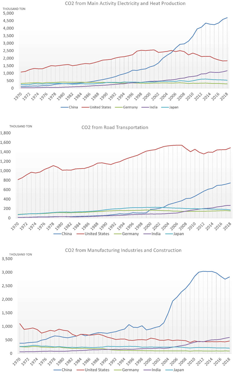
FIGURE 1. Carbon emissions in different sectors.

In summary, to control energy consumption and carbon emission, the prior sectors to pay attention to are residential electricity and transportation, both of which are closely related to residents’ daily lives. In classical consumption theory, the life cycle phase of the family is critical, so our study takes the age structure as the entry point for analysis.

1.2 Impacts of Carbon Emissions on Climate: Frequent Extreme Weather Events and Difficulty in Adapting to Environmental Temperatures for the Elderly Population

According to the world economic forum, extreme weather events are becoming increasingly frequent and more severe due to climate change (Gleason et al., 2008; Stott, 2016). They are already a harsh reality for communities worldwide. Between 1998 and 2017, an estimated 526,000 people lost their lives due to extreme weather, while economic losses amounted to $3.47 trillion (in PPP), according to the climate risk report by Germanwatch. In relative terms, poorer developing countries suffer a much more significant impact from these natural disasters, and the report has highlighted their vulnerability to the planet’s changing climate.

Another paper from The Lancet by Zhao et al. (2021) has even more striking findings. Their results indicate that abnormally high and low temperatures are occurring more frequently as climate change accelerates, and these temperature anomalies will cause an additional 5 million deaths per year globally. The cross-nation study analyzed mortality and temperature data from 750 sites in 43 countries between 2000 and 2019, with global temperatures rising by 0.26°C per decade during the survey cycle. It is estimated that globally, 9.4% of deaths per year are caused by extreme cold and hot temperatures, equaling 74 excess deaths per 100,000 people. Heat-related deaths increased by 0.21%, as deaths associated with colder temperatures decreased by 0.51% over the 20 years as the planet warms.

Moreover, over 50% of the excess deaths occurred in Asia, particularly in low-lying and crowded coastal cities in East and South Asia. This result underscores how daunting it is for Asian countries to reduce the adverse effects of temperature on local population health and the enormous challenges to their health care systems. New results strongly suggest that non-optimal temperatures are one leading cause of disease burden for population health.

At the same time, there is a new trend in global demographics as the underlying driver of the economic phenomenon of energy consumption and carbon emissions - namely, population aging. The proportion of the world’s population over 60 almost doubled from 2015 to 2050, from 12 to 22%. By 2050, there will be 120 million older people in China alone and 434 million older people worldwide. By 2050, 80% of older people will be living in low- and middle-income countries, as shown in Figure 2.

FIGURE 2

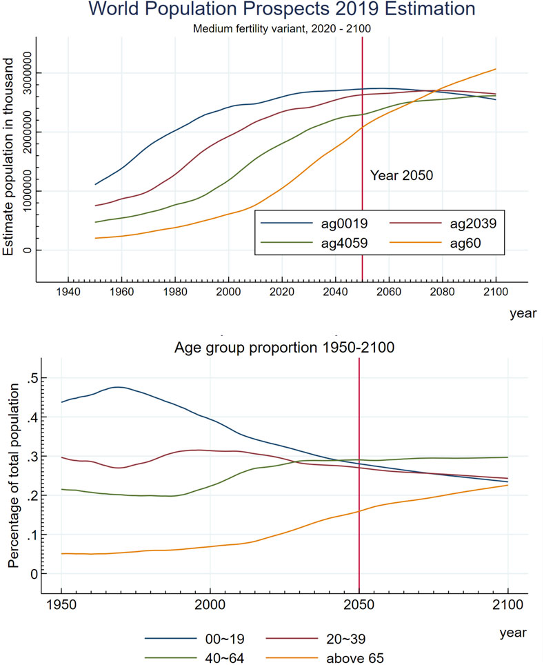
FIGURE 2. The world population aging trend with estimation from WPP 2019. Here, red line stands for the year 2050.

As United Nation’s < world population ageing highlight 2019> indicates, the aging trend developed faster in Eastern and South-Eastern Asia, Latin America, and the Caribbean. This geographic distribution coincides with the geographic distribution of excess mortality due to heat and cold, raising the more demanding challenge that regions with low-temperature comfort levels have the highest proportion of temperature intolerant populations, and that this problem can only be solved by regulating ambient temperatures, leaving these countries with less leeway to reduce carbon emissions.

Considering what potential impacts the increase in elderly proportion may impose on total carbon emissions, one intuition is that energy consumption will become lower if the elderly is less involved in economic activity. Thus, carbon emissions will decrease, and population aging also implicitly decelerates economic growth, especially in terms of innovation or labor supply; consider the lackluster society where most citizens are elderly and in need of care as the extreme case, the intuition is easy. At the same time, we should realize that the increase in extreme weather events and their challenge to the environmental resilience of the elderly population will take this prognosis of impact in an uncertain direction. We cannot say whether the reduction in carbon emissions due to the rate of increase in the share of the elderly population relative to young adults will have a more substantial impact or the increase in carbon emissions due to the increased energy demand of the elderly population due to unusual weather. Our study answers this question by verifying that carbon emissions from cooling and heating needs from the elderly population also need to be taken into account.

While increasing the supply of electricity and more scientific deployment of electricity resources is certainly one approach, one aspect that has been neglected in past studies and policies is how to achieve energy savings while maintaining the proper ambient temperature effectively. In previous studies, the discussion of carbon emissions from buildings has focused more on the carbon emissions associated with the production of the various raw materials used in buildings. However, our study considers the carbon emissions from the intersection of building use and residential life. The potential of energy-efficient buildings to reduce emissions is not negligible and can be an essential reduction channel. With findings by Balaras et al. (2005), comparison with the heating energy consumption of 193 European residential buildings from five countries shows that 38% of the audited buildings had annual heating energy consumption higher than the European average (174.3 kWh/m²). In developed countries, where residential energy consumption accounts for about 1/3 of total energy consumption, households are significant contributors to GHG emissions and global warming. Over the past decades, there have been significant improvements in building energy efficiency by introducing new building codes and the construction of low-energy buildings.

1.3 Literature Reviews

There are two main theoretical explanations for the discussion on population and carbon emissions, one is a modified version of the PAT model, the STIRPAT model, and the other is the EKC curve. The main difference between the two theories is whether the relationship between income and carbon emissions is linear or quadratic and whether the population coefficient is different from unity.

As for the determinants, the scientific community has conducted many analyses on carbon emissions, and it is generally accepted that CO₂ emissions are determined by the level of technology, affluence, energy structure, economic structure, and population structure. Early studies considered energy consumption as the primary source of carbon emissions and did not consider the influence of population and technology (Shi, 2003). Other studies consider both population, technology, and the economy as essential factors influencing carbon emissions (Englman, 1994; Cole et al., 1997; Meyerson, 1998; Schmalensee et al., 1998), and further argue that the impact of these factors is heterogeneous among countries (Shi, 2003). Ever since the STIRPAT model, a large number of studies have started to use multi-country samples. Dietz and Rosa (1997), York et al. (2003a) conclude that the elasticity between carbon emissions and population growth is about 1, Shi (2003) calculates elasticities between 1.41 and 1.65, Fan et al. (2006) shows that the effect of economic growth is the largest for all countries, while the effect of the population share between the ages of 15 and 64 is the smallest. Li et al. (2011) used a combination of PATH analysis and STIRPAT model to study the China sample and found the elasticity coefficients of the urbanization rate is positive (Ji and Chen, 2017).

Liddle has studied the environmental impacts of population age structure on carbon emissions in Liddle and Lung (2010), Liddle (2014). In Liddle (2015), residents are divided into different age groups. The conclusions are consistent that the U-shaped effect of the age structure on carbon emission exists, as though the relationship may change with the different indicators for carbon emission. Other similar studies have examined the heterogeneity effects of factors with regional data such as Pakistan (Shahbaz et al., 2017), Guangdong (Wang et al., 2013), Taiwan (Yeh et al., 2016), the Middle East (Tarazkar et al., 2020), Fujian (Su et al., 2020), and South Korea (Kim et al., 2020), and OECD (Shafiei and Salim, 2014), respectively.

The most recent literature, on the other hand, makes the extension of the STIRPAT model based on climate and socioeconomic factors, energy intensity (Poumanyvong and Kaneko, 2010; Kais and Sami, 2016; Hao et al., 2016; Vélez-Henao et al., 2019), trade openness (Kais and Sami, 2016; Wang and Zhang, 2021), industrialization (Wang et al., 2020), urbanization (Ghazali and Ali, 2019; Salim et al., 2019; Ahmed et al., 2020), and energy mix (Sheng and Guo, 2016). Considering the mobility of greenhouse gases, spatial models such as Spatial Durbin might be more suitable (Lv, Chen, and Cheng, 2019).

It can be concluded from above that previous studies mainly focus on the impact of socioeconomic development on carbon emissions. However, the factors affecting carbon emissions can be complex, climate changes are involved though seldom tested. As York et al. (2003b) point out, the climate type of the country impacts the magnitude of different determinates’ carbon elasticity, climate factors such as precipitation and mean temperature should be included in the analysis. However, little attention has been paid to the impact of environmental factors, including climate change. Therefore, this paper coordinates climate variables, and economic and age structure factors into the STIRPAT model to reveal the driving mechanism of carbon emissions under the combined effect of climate factors and socioeconomic factors.

In this paper, the STIRPAT model is modified to examine demographics and climate impact. Based on the theory of the household consumption life cycle, we divided the population into four age groups and verified the heterogeneous impact of age on carbon emissions in the macro-level. From the perspective of the earth science model, this study discussed the climate heterogeneity in the relationship of population-carbon emission. Three long-term and short-term climate indicators, Temperature Anomaly, Precipitation, and Degree-Days, are used to verify their impact on carbon emission, and the discussion based on Köppen grouping is also added. It is confirmed that the increase of heat and electricity carbon emission is due to the elderly population having declined physical adaptability, resulting in more air conditioning energy demand. With the population aging becoming a global issue, the role of energy-saving buildings and green buildings concept in carbon emission reduction should be paid attention to.

The rest of the paper is arranged as follows: Section 2 reviews literature with micro-level evidence to provide explanations why age structure and climate factors should be considered in carbon STIRPAT models and deduction of the corresponding seemingly unrelated equation sets; Section 3 introduces the climate indicators used and various sources of meteorological data; Section 4 presents the empirical results of the model, results interpretation, and heterogenous analysis of emission patterns with various robustness checks; Section 5 concludes the main findings and suggests that national differences in economic development stages should be considered in international climate cooperation to make the plan more fair. A new standard for energy efficient buildings should be set with insulation upgrade projects funded by governments to reach a possible reduction from the energy sector.

2 The Climate-Extended STIRPAT Model

2.1 Classic STIRPAT Model

Ehrlich and Holdren (1971) first proposed the IPAT model (I=PAT) to measure the impact of human activities on the environment, which specifies that environment quality (I) is influenced by three factors: the population (P), affluence (A), and technology (T). The IPAT model is restricted in use as it relies on solid presumptions (Shi, 2003). Dietz and Rosa (1997) proposed the stochastic version of IPAT as STIRPAT, then York et al. (2003a) refine the STIRPAT model. Indicators such as modernization (urbanization and industrialization) are also considered, and climate is found to have a multiplier or diminutive effect on factor influences.

$I=P\text{*}A\text{*}T(1)$

Here $I$ denotes environmental impact, $P$ denotes population, $A$ denotes wealth or per capita consumption, and $T$ denotes the impact of technology, usually employs carbon intensity as an indicator. Notice that the input factors of the IPAT model are limited to the same exponent, which creates difficulties for practice, so the STIRPAT model improves the applicability of the IPAT model by considering a stochastic form as:

$I_i={\alpha }_i\times P_i^b\times A_i^c\times T_i^d\times {\epsilon }_i(2)$

The subscript $i$ represents the cross-sectional unit (i.e., country or distinct), $\alpha$ is a constant, b c d are the parameters to be estimated, and ${\epsilon }_i$ is the error term. Rewrite the above equation in log-linear form, the estimated parameters can be considered as the corresponding elasticities.

$Ln{I}_i=Ln{\alpha }_i+bLn{P}_i+cLn{A}_i+dLn{T}_i+Ln{\epsilon }_i(3)$

In practical application, $I$ is generally taken as CO₂ or GHG emissions, and researchers continue to isolate various control variables from ${\epsilon }_i$. Our study also followed this idea, and reasons for separating age structure and climatic factors are described below.

2.2 Why Age Structure Also Matters in Determining Carbon Emission

How does population influence energy consumption and thus total carbon emissions? We divide it into two channels: Aggregate effects and structural effects. In addition to the aggregate population effect, the main channel through which the population affects carbon emissions is the household energy consumption behavior (if we do not limit the number of household members), which directly consumes energy and generates carbon emissions, mainly through electricity and transportation. Much literature has examined the impact of population age structure factors on energy consumption, while minor literature directly discusses the relationship between overall population age structure and carbon emissions. Studies on micro-level survey data sufficiently demonstrate that different household characteristics (e.g., age of head of household, number of household members) result in different economic activity patterns.

An earlier study by Fritzsche (1981) on American household energy consumption patterns mainly considered that income, age structure, number of family members, and consumption habits fluctuated with household life stages. The study found that household energy consumption rises and then falls with the birth of a child, declines after the child leaves home as an adult but remains higher than in the younger years until there is only one spouse and energy consumption rapidly falls below the single stage. The total energy consumption pattern is an inverted U-shaped distribution, with the right side of the U higher than the left side. It is also noted that people who suffer as summer temperatures rise are also those who suffer most when winter temperatures fall. There is a negative correlation between the width of people’s thermal preference range and their residential energy consumption.

Leading us to wonder whether energy consumption would be greater if the proportion of the population having a relatively narrow (ambient temperature) thermal preference range raises as older people tend to be less able to function physically.

Follow-up scholars have also studied the effect of population age structure on energy consumption based on data from more countries. However, a unified conclusion has not been reached about the energy consumption of different age groups and whether aging reduces energy consumption and carbon emissions. For example, York (2007) argues that populations with a higher proportion of older people (older cohorts) consume more energy than populations dominated by younger people, which differs from the findings of Fritzsche (1981). We believe that environmental temperature suitability may be a vital source to explain the differences in research findings. York’s study also used the STIRPAT model and data from 14 EU base countries for 1960–2000 to estimate the impact of demographic and economic factors on energy consumption. His result indicates that countries with a higher proportion of older people consume more energy than other countries. However, the demographic variable in the study refers to the percentage of the population over 65 years old, not the age structure of the entire population by age group. At the same time, the results cannot completely exclude the effect of low fertility, which we know can change the distribution of family structure (size) in society. To explain the differences, we need data support at a more micro level, in two sectors, looking for supporting literature evidence according to two components: home activities and transportation, where households consume energy, respectively. According to the IPCC’s classification of emission sources, this study selected three sectors to examine the environmental impact of the population structure from three channels: total carbon dioxide emissions, transportation carbon emissions, electricity, and heat consumption carbon emissions.

The demographic structure can be an important factor affecting a country’s carbon emissions. Detailed discussion is provided in the subsequent sections, but we can start by giving a presumption based on the effect of household size composition on total carbon emissions. People in different age groups have different incomes and consumption behaviors. This study divides residents into four age groups: 20–34 years old, 35–49 years old, 50–64 years old, and over 65 years old. Such grouping considers the economic activities in different life cycle stages are different, and the number of family members is also different (Liddle and Lung 2010). The age group led structural difference is explained in Table 1; this classification of age groups is aligned with the reality of most developed and developing countries.

TABLE 1

TABLE 1. Household life cycle and different age groups

Usually, the 35- to 49-year-old population has the largest average family size and should show lower energy intensity. People over 65 stay at home more, have lower transportation needs, and are sensitive to ambient temperature. They may consume more electricity for heating and cooling. Young and middle-aged people (20–34 years old) are energetic, and their wealth is in the accumulation stage, but their household expenses are lower, consumption higher, travel more, and they may have the highest per capita carbon emissions, so in general the hypothesis is proposed as follows:

H1.a: Arranged age groups in order from young to old, 20–34 years old, 35–49 years old, 50–64 years old, and over 65 years old, there is an inverted U-shaped relationship between the share of each population age group and total carbon emission, the higher the share of middle-aged people, the higher the total carbon emission, while the carbon emission elasticity of the share of young and old people is lower.

2.2.1 Micro-Evidence of Household Transport Energy Consumption Pattern

Age is essential for travel distance because older people and children do not travel for work (Sovacool et al., 2018). In addition, travel is also influenced by gender, as women work more often than men in or near downtown areas with good access to public transportation, while men often work in manufacturing plants far from downtown areas (Vilhelmsson, 1988). Carlsson-Kanyama and Lindén (1999) investigated the travel patterns of different socioeconomic groups in Sweden. The results show that older people, low-income people, and women do not generally travel extensively. Middle-aged people, high-income earners, and men travel much farther. Energy consumption varies considerably by mode of travel, with automobiles being the dominant mode of transportation for all demographic groups, airplanes being used primarily by high-income earners and men, and public transportation is used primarily by young people and women. Men between the ages of 35 and 54 travel the farthest distance, while older women travel less than 1/3 of that distance. Even young children between the ages of 6 and 14 travel farther than older women, and children are the most frequent travelers in various vehicles for commuting to and from school and leisure activities.

Here we determine that there may be an inverted U-shaped relationship between age structure and transportation energy consumption, with travel and trips increasing incrementally with income at younger ages, peaking at middle-age and older ages, and decreasing to a minimum at older ages.

H1.b: From young to old, there is an inverted U-shaped relationship between the share of each population age group and transport carbon emission, middle aged travels more and elderly less.

2.2.2 Micro-Evidence of Residential Energy Consumption Pattern

Yun and Steemers (2011) used the 2001 US Residential Energy Consumption Survey (RECS) to analyze how human behavioral, physical, and socioeconomic factors affect household cooling energy consumption. They found that the influence of human behavioral factors is more significant than that of climatic factors, and they argue that there is a relationship between these variables, as shown in Figure 3. As we can see, the age and income of the householder affect all these variables and directly affect cooling energy consumption. However, their empirical part uses the linear form function to verify the impact of age, and this setting may be problematic considering that the total energy consumption of a household may present a curve process that rises and then falls as householder’s age changes. So, the significant negative correlation between age and energy consumption in their findings deserves further verification.

FIGURE 3

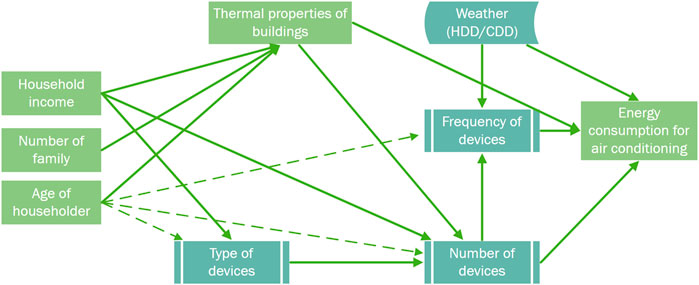
FIGURE 3. Household features and air conditioning energy demands.

More detailed summary of the influencing factors is presented in Bhattacharjee et al. (2012). The study reviews approximately 50 literatures on the factors influencing energy consumption in the residential sector. Pachauri (2004) used micro-level household survey data from 1993–1994 in India and showed that the age of the householder and energy consumption were positively correlated, with per capita energy demand being about 7% higher when the householder was between 25 and 29 years old than when the householder was younger than 25, and increases to 13% when the age of the householder is over 50.

Much of the energy used by older adults is related to their health and comfort, and some of the reasons for the increase in per capita energy consumption with age are the lack of information and knowledge about energy conservation, the inertia to make changes, and the importance of subjective well-being. The energy consumption required to achieve environmental well-being is undoubtedly an essential factor influencing energy consumption and carbon emissions in old age. Long et al. (2019) investigated the relationship between household consumption and energy demand at the urban level using an urban-scale input-output model and an urban residential consumption inventory in Tokyo, Japan. Furthermore, the age grouping of the study is very detailed, with a 5-year interval grouping between 30 and 69 years old, and an apparent change in life-cycle energy consumption habits can be observed, and their findings show that (1) household emissions vary significantly across age groups; per capita emissions are generally higher in older households; (2) temperature decline is the main reason for the increase in emissions in older households, while this is not a significant factor; and (3) high per capita emissions in older households indicate inefficient energy use by senior citizens, which strongly suggests that aging societies will face long-term emission increases if appropriate measures are not taken.

H2: The coefficient of the cross-term between the aging dummy and DD is positive, considering the existence of the greater need to regulate the ambient temperature of the elderly.

The literature evidence suggests that culture is also an important consideration. As with all other analyses of consumption habits, differences brought about by culture and social convention also encompass energy consumption habits. For example, the Confucian cultural circles, known for their frugality, may present different patterns from Westerners (Yang and Wang, 2020). Chen et al. (2013) used data from a survey of residents in Hangzhou, China, to investigate the causes of increased building energy efficiency but not decreased energy consumption and found that the occupants’ age had a more significant impact on energy consumption than income. Unlike previous results in the literature, the study found that older residents showed more frugal behavior patterns than younger people. This opposite result, we believe, may be related to China’s particular economic development history and culture; the country is still in the materially scarce stage during the early years of older residents. The process of changing consumption habits is gradual, so it cannot be as rapid as the change in economic data, for which numerous literatures can provide relevant evidence on cautious consumption habits of the Chinese.

Still, most studies support the inverted U-shaped relationship between the age of the householder and household energy consumption. Leahy and Lyons (2010) proved 45- to 65-year-old householders use more electricity than those aged 35–44. In addition, electricity consumption decreases when the householder gets older than 64. Belaïd (2016) explores the determinants of household energy consumption using data from the French National Housing Survey of 43,000 households in 2006. Energy consumption increased by 1% for every 10-year increase in the age of the householder. Energy consumption increases rapidly in the early years of one’s life, and it becomes more gradual as the householder gets old.

H1.c: From young to old, there is an inverted U-shaped relationship and uplifted tail between the share of each population age group and heat and electricity carbon emission.

Therefore, most studies showed this inverted U-shaped trend of the age-carbon emission relationship, while a few reached different conclusions, making us realize that the analysis of this issue must be seen in the context of the specific development history and the particular cultural factors of a given country, so a relevant heterogeneity analysis is also set up in the empirical section to analyze how these shared characteristics and features arise.

2.3 The Climate Types and Influences on Carbon Emission

The previous section’s micro data on household energy consumption pathways and influencing factors also show that climate (especially temperature) is undoubtedly an essential factor in energy consumption. However, there is little literature on this issue from a macro perspective - what role does climate play in carbon emissions? On the one hand, we believe the problem may come from the difficulty to obtain data, as the processing of climate data is complex and there is no uniform method to choose an accurate metric, for example, how to weigh a comprehensive climate indicator in a large country; on the other hand, there is a lack of theoretical basis for the detailed influence mechanism. The process might be non-linear, and the mechanism is more complex than simply add-up. We can only assume its functional form than judging it directly. Nevertheless, it is worthwhile to address the relation between carbon emissions, climate, and demographics, as comparative studies at the national level are too scarce compared to behavioral studies at the micro-level.

2.3.1 The Köppen Climate Types

If we consider the spatial mobility of GHG and the heterogeneity of energy demand, the climate is an important aspect that cannot be ignored. Although studies such as York et al. (2003b), Liddle and Lung (2010) pointed out its importance, their analysis was limited to group comparisons, such as tropical vs. non-tropical areas. Until recently, studies such as Yang et al. (2018) used actual climate indicators such as precipitation, temperature anomaly, and cooling/heat degree days. To address the issue of climate influence on the heterogeneity of demography-carbon emission relationship in previous literatures, it is necessary to define what is climate and consider which classification standard can be used to distinguish it. This required the chosen method to be publicly acknowledged, containing crucial and simple climate variables to which carbon emissions are closely related.

Based on the above criteria, this study selects the Köppen climate type classification. It provides an efficient way to describe climatic conditions with parameters such as temperature and precipitation and their seasonality with a single metric. It also has the widest acceptance in various studies and standards worldwide as the climatic conditions identified are ecologically relevant, giving us a solid basis for studying human activities and associated carbon emissions in the ecological context.

The Köppen classifies the global climate according to its latitudinal position, from the equator to the poles, into five major climate regions: A. Tropical (tropical climate), B. Arid (dry climate), C. Temperate (subtropical climate), D. Continental (temperate and subtropical climate), and E. Polar (polar climate). Each major category can be subdivided into a number of subcategories, and the global climate is divided into 31 subcategories, each of which is graded in detail using two to three letters of the alphabet. The detailed global classification is shown in Figure 4.

FIGURE 4

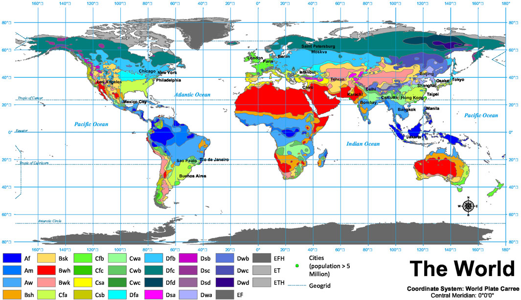
FIGURE 4. The Köppen climate types map with (1901–2000) grid datasets.

Average precipitation and temperature are strictly essential to Köppen classification. So, along this line of thinking, we choose three key climate indicators affecting carbon emissions, namely: annual mean precipitation (PRE), annual degree-day (DD), and temperature anomaly (TA). Detailed in Section 3, the calculation of PRE and DD is derived from the accumulation of short-term terms that distinguish between climate types and the actual weather for that year in a certain country. The annual precipitation indicator is direct to classify the climate type of country and DD not only captures and represents the daily temperature variation at a given location more effectively than the annual mean temperature, but also straightforwardly represents the building energy demand. Meanwhile the TA, a sign of long-term climate change by definition, reflects the degree of change in a country’s climate relative to the pre-industrial era, is a good implication for how bad the global warming situation becomes, and it is also set as IPCC’s goal for comparison with the Global Carbon Reduction Cooperation. The mechanisms by which the three channels affect carbon emissions is described in the next section.

With the theories model by 2021 Nobel Prize winners in Physics, Syukuro Manabe and Klaus Hasselmann, the relations can be generalized below, and specific forms of each equation with the mechanism hidden behind in the following, and briefly framed as shown in Figure 5. Hasselmann (1976) considered the ecosystem of earth consisted of two parts: rapidly varying “weather” system (essentially the atmosphere) and a slowly responding “climate” system (the ocean, cryosphere, land vegetation, etc.). Here we used TA as the proxy for slowly changing climate, and the annual sum of DD and PRE is used as the proxy for rapidly changing weather systems.

$\{\begin{array}{c}C={\varphi }_1\left(TA\right);long term, Thermal radiation equation\\ C={\varphi }_2\left(PRE\right);short term,Carbon sink role of nature\\ C={\varphi }_3\left(DD\right);short term, General circulation model of the atmosphere\end{array}$

FIGURE 5

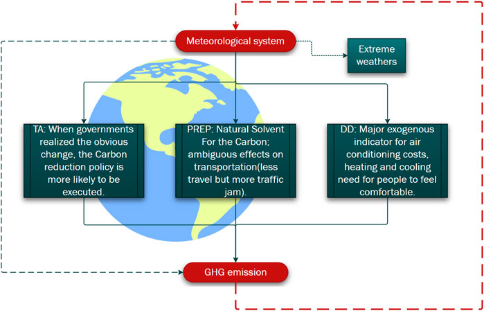
FIGURE 5. The interactive mechanisms between carbon emission and the stability of the meteorological system, in accordance with the box diagram of the basic structure of the mathematical model of global climate in Syukuro and Stouffer (1980).

2.3.2 The Climate Mechanism on Carbon Emission

According to the National Oceanic and Atmospheric Administration (NOAA), TA refers to temperature deviation from the reference value or long-term average value. For the studies related to global warming issues, the reference value is often set at the pre-industrial level, and the latest benchmark is the land and ocean surface average temperature from 1901 to 2000. A positive TA value indicates the observed temperature in certain place is higher than the reference value. In Figure 6, the value of temperature rises in major cities around the world since the 21st century is shown. It can be observed that the surface temperature rise in higher latitudes is more pronounced than in lower latitudes. This is one of the serious consequences of global warming.

FIGURE 6

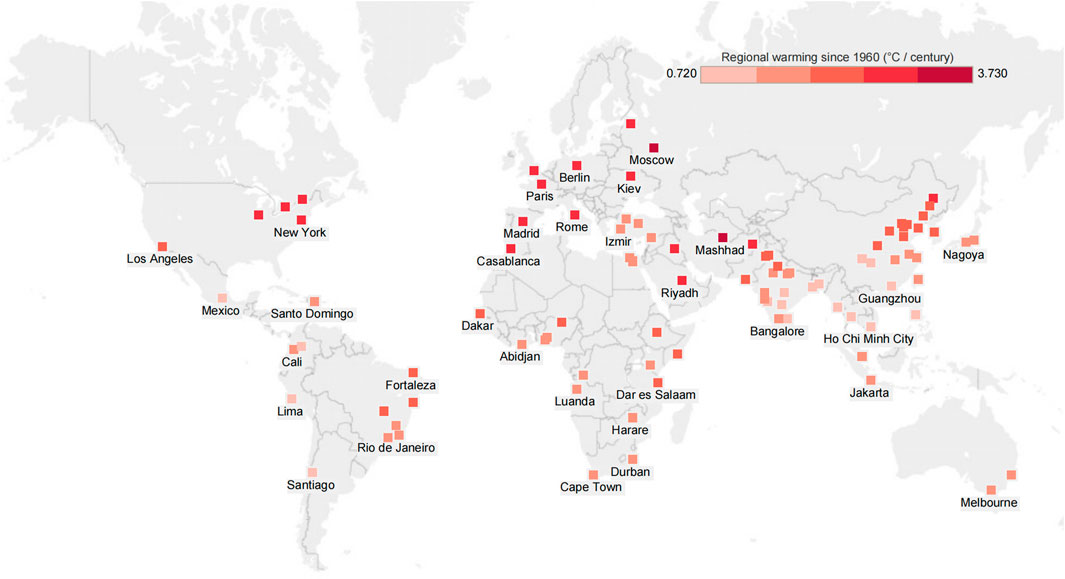
FIGURE 6. Temperature appreciation in major cities in the 21st century (largest cities local temperature change use 1900 as the base line) with original data from Berkeley Earth Lab.

TA (long-term climate change term) is the main indicator of climate change in global meteorological cooperation, as it is the most direct representation of the long-term impact of carbon emissions from human activities on climate. TA affects the possible lag effect between the implementation of policies that specifically produce effects; at the same time, the larger the TA value, the greater the probability of countries experiencing extreme weather events, and the stronger the willingness of governments to carry out carbon emission reduction after considering economic and human losses. The hypothesis is proposed as follows:

H3: As TA increases, the total carbon emissions should decrease, this channel may have a lagged effect and a threshold effect related to the degree of economic development.

In meteorology, precipitation is defined as any product of the condensation of atmospheric water vapor that falls under gravitational pull from clouds. The main forms of precipitation include drizzling, rain, sleet, snow, ice pellets, graupel, and hail. As for the channel of precipitation on carbon emission, there are two paths, climate ecosystem and human activities: for climate ecosystem, precipitation itself circulates in the global climate system, and the deposition of dissolved organic carbon and carbonate will complete the role of terrestrial and marine carbon sink (Fang et al., 2017). Second, precipitation affects plant physiological processes in the ecosystem. The growth of natural vegetation is closely related to the increase of precipitation and humidity, thus affecting plant carbon sink (Nemani et al., 2002; Gemechu Legesse et al., 2021).

Another chain is about the impact of precipitation on carbon emissions of human activities, such as traffic carbon emissions. On the one hand, due to inconvenient travel, accidents, delay rates, and other reasons (Zhan et al., 2020), rainy or snowy days have a negative impact on highway traffic volume and public transport passenger volume, and the decline on weekends is more significant than that on weekdays (Changnon, 1996) The report issued by US Department of Transportation shows that the rain, snow, and precipitation process affects the free-flow speed and capacity of traffic, and these parameters will change with the change of precipitation intensity (Hranac et al., 2006 and United States. Federal Highway Administration. Road Weather Management Program. 2016), When the traffic flow pattern changes suddenly or the number of vehicles increases, especially during peak hours and special events, the emissions from roadsides and intersections will be affected. Vehicles queuing at traffic intersections spend a long time in idle driving mode and produce more pollutant emissions per unit time (Gokhale and Pandian, 2007).

So, in general, PRE (short-time weather term accumulated in year) is the representative indicator of annual precipitation intensity and quantity, when its value becomes larger, the carbon contents in the air would reduce due to the carbon sink effect of water and plants in the earth’s ecosystem; on the other hand, rain and snow days affect people’s traffic trips, while the traffic volume goes down, the traffic conditions deteriorate and this may lead to traffic congestion and increase carbon emission per unit time due to changing traffic flow patterns. The overall influence is ambiguous. The research hypothesis is proposed as follows:

H4: As the PRE value increases, the total carbon emission decreases (because of the enhanced carbon sink effect of water and plants); however, the direction of the impact of PRE on transportation carbon emission is uncertain; total traffic volume will decrease, but carbon emission may increase due to congestion.

Defined by the US Environmental Protection Agency, and being one of the key set of indicators related to the causes and effects of climate change, DDs measure the difference between outdoor temperatures and what people typically consider comfortable indoor temperatures. It is calculated as the absolute value of the difference between the average daily temperature and the equilibrium point temperature (15.6°) of which the definition of comfortable temperature varies from agency to agency, with NOAA still using the standard of 65°F, and Energy CAP’s survey for modern buildings determining a comfortable temperature of 60°F. The degree-day level indicates how much energy people may need to use to heat and cool their homes and workplaces. It is first introduced by Thom (1952), was widely employed as a measurement of climate change (Pardo et al., 2002; Mirasgedis et al., 2006; Pilli-Sihvola et al., 2010), providing an understanding of how climate change affects people’s daily lives and financial situations.

DD (short-time weather term accumulated in year) measures the degree of ambient temperature suitability for people, which will directly affect the frequency and intensity of use of ambient temperature regulation equipment such as air conditioners. In addition, with analysis in Section 2.2.2, this consumption habit varies with the age of residents, so it will also vary with the proportion of the population of each age group, but overall, the positive impact is predictable. So, the research hypotheses for DD is proposed as follows:

H5: The larger the DD, the more the total carbon emission, the more the heat and power sector carbon emission, and there may be an interaction effect between the effect of DD and the percentage of age grouping.

2.4 How the Climate and Age Structure Can Be Incorporated in a STIRPAT Model

With the above analysis on the impact mechanism of demographic structure - carbon consumption habits and carbon in global meteorological systems, the original STIRPAT model formula of Section 2.1 can be rewritten as:

$Ln{I}_{it}\mathrm{\approxeq }Ln{\alpha }_i+b_{1}Ln{\left(1-{\displaystyle \sum A{G}_{\left(m,n\right)}}\right)}_{it}+b_{2}ln{P}_{it}+cLn{A}_{it}+dLn{T}_{it}+{\epsilon }_{it}$

Assuming that 1-x is small enough, here we have $ln(1+x) \sim x$ according to the principle of equivalent infinitesimal substitution, and the original equation becomes:

$Ln{I}_{it}=Ln{\alpha }_i+{\displaystyle \sum b_{k}A{G}_{\left(m,n\right)it}+}{b}_2\mathit{ln}{\mathit{p}}_{\mathit{it}}+cLn{A}_{it}+dLn{T}_{it}+{\epsilon }_{it}$

The effects of climatic factors (precipitation, temperature anomalies, degree-days) on total carbon emissions are included in the original error term part considered their linear relationship with carbon emissions, noted here the coefficients before age ratio stands for the deviation degree of different age group’s carbon emission elasticity from the average carbon emission elasticity of the whole population, the corresponding estimating equation is:

$Ln{C}_{it}={\alpha }_i+{\displaystyle \sum b_{k}A{G}_{\left(m,n\right)it}+{\text{β}}_{2}ln{P}_{it}+{\text{β}}_{3}Ln{A}_{it}+{\text{β}}_{4}Ln{T}_{it}+{\text{β}}^{\text{'}}{\text{X}}_{\text{control}}^{\text{'}}+{\text{β}}_{6}lnD{D}_{it}+{\text{β}}_{7}PRE+{\beta }_{8}TA+{\epsilon }_{it}}$

2.4.1 The SURE Setting for Extended STIRPAT Model

Considering that there are 247 countries and regions in the world, each country has its own carbon consumption equation. As for our sample, there should be 150 equations to describe the actual pattern. The influencing factors of carbon emission in each country may be different, that is, some variables do not exist in all models, and different influencing factors (explanatory variables) may be included in the equations of different countries, although the carbon emission patterns among countries with close geographical location or similar development may have the same characteristics. Obviously, the carbon emission equations of various countries seem independent, but they exist in the same earth ecosystem, and there is some connection between them. This relationship can be explored by testing the joint distribution of disturbance terms. It is considered that the simultaneous correlation of error terms is reasonable, that is, these equations seem independent and uncorrelated, but they are only seemingly unrelated (Biørn, 2004). A.

A typical SUR model is constructed as follows, consisting of M multiple regression equations.

$y_i=X_i{\beta }_i+{\epsilon }_i, i=\mathrm{1,2,3}\dots ,M$

Here $y_i$ is T-dimension vector with elements $y_{ti}$, $X_i$ is $T \times K_i$ matrix represents explanatory variable’s T-th observation in the i-th equation; and ${\beta }_i$ is ki vector, ${\epsilon }_i$ is T disturbance vector with the expanded form like:

$\left(\begin{array}{c}{y}_1\\ y_2\\ \begin{array}{c}⋮\\ y_m\end{array}\end{array}\right)=\left(\begin{array}{ccc}{X}_1& 0& \begin{array}{cc}\dots & 0\end{array}\\ 0& X_2& \begin{array}{cc}\dots & 0\end{array}\\ \begin{array}{c}⋮\\ 0\end{array}& \begin{array}{c}⋮\\ 0\end{array}& \begin{array}{cc}\begin{array}{c} \ddots \\ \dots \end{array}& \begin{array}{c}⋮\\ X_m\end{array}\end{array}\end{array}\right)\left(\begin{array}{c}{\beta }_1\\ \begin{array}{c}{\beta }_2\\ ⋮\end{array}\\ {\beta }_m\end{array}\right)+\left(\begin{array}{c}{\epsilon }_1 \\ \begin{array}{c}{\epsilon }_2\\ ⋮\end{array}\\ {\epsilon }_m\end{array}\right)$

Moreover, for estimation it requires that the variance of all ${\epsilon }_{ti}$ is constant, the contemporaneous covariance between ${\epsilon }_{ti}$ and ${\epsilon }_{tj}$ is constant for all time, and intertemporal covariance of ${\epsilon }_{ti}$ is zero. The estimation should be implemented with multistep maximum likelihood method (Minh Nguyen and Hoa Nguyen, 2010). Here we have carbon emission from different sectors, if we write the equations in pairs, then:

$\{\begin{array}{c}Ln{C}_{it}={\alpha }_i+{\displaystyle \sum b_{k}A{G}_{\left(m,n\right)it}+{\text{β}}_{2}ln{P}_{it}+{\text{β}}_{3}Ln{A}_{it}+{\text{β}}_{4}Ln{T}_{it}+{\text{β}}_{5}U{R}_{it}+{\text{β}}_{6}lnD{D}_{it}+{\text{β}}_{7}PRE+{\beta }_{8}TA+{\epsilon }_{it}}\\ LnT{C}_{it}={\alpha }_i+{\displaystyle \sum b_{k}A{G}_{\left(m,n\right)it}+{\text{β}}_{2}ln{P}_{it}+{\text{β}}_{3}Ln{A}_{it}+{\text{β}}_{4}Ln{T}_{it}+{\text{β}}_{5}U{R}_{it}+{\text{β}}_{6}PR{E}_{it}+{\epsilon }_{it}}\\ LnE{C}_{it}={\alpha }_i+{\displaystyle \sum b_{k}A{G}_{\left(m,n\right)it}+{\text{β}}_{2}ln{P}_{it}+{\text{β}}_{3}Ln{A}_{it}+{\text{β}}_{4}Ln{T}_{it}+{\text{β}}_{5}UR+{\text{β}}_{6}lnDD+{\text{β}}_{7}lnDD\times D_{ol{d}_{it}}+{\epsilon }_{it}}\end{array}$

The subscript it represents the ith country and the tth period, CO2 is the total carbon emissions, and POPU, $A{G}_{(m,n)}$, A, and T are the total population, proportion of different age groups, GDP per capita, and energy intensity (energy consumption per unit of output value). The constant term α is other characteristic factors of the country, ${\epsilon }_{it}$ is the error term, TO represents the degree of openness to trade (measured as the proportion of GDP in total import and export value), UR is the urbanization rate (the proportion of urban population to the total population), and PRE is annual precipitation, TA is the annual average temperature abnormal value (based on the pre-industrial era of 8.5°C as the standard, NOAA), DD is the number of degree days, the sum of HDD and CDD, and refers to a period of time (year or season) where the daily average temperature is higher accumulated degrees below 60 or 65°F (18.3°C) represent residents’ demand for cooling and heating. The equation for analyzing traffic and electricity carbon emissions is similar but with minor modification according to the mechanism and assumptions. The same symbol meanings hold as above, EC denotes residential electricity carbon emissions, $D_{ol{d}_{it}}$ is a dummy variable for aging society according to the UN classification criteria, noting that the proportion of a country’s population aged 65 years and older exceeds 7% as 1, and 0 for the rest.

2.4.2 Threshold Model for Determining Carbon Emission Peaking by Country

Considering that the carbon emission stage of various countries may have differentiated with economic development and industrial structure changes, namely, some developed countries may have reached the peak of carbon emission, while some developing countries are still in the rising stage before the peak. If the judgment standard is set as the growth rate of carbon emissions becomes lower than the growth rate of GDP, most developed countries may have already reached the carbon emissions peak from the 1970s–1980s and transferred the high input and high pollution enterprises outward by participating in the global value chain. From previous literatures, there are four main determining methods for carbon emissions peak: LMDI driving factor judgment, various sector carbon emission trends, carbon decoupling index, and Environmental Kuznets Curve (EKC). Considering that other methods have high requirements for the analysis of a country’s own characteristics, in order to be comparable, this study uses the EKC method to judge whether a country’s carbon emissions peak or inflection point has been reached.

Besides, taken the environmental Kuznets hypothesis into consideration, for countries at different income levels, the relationship between demographic structure and carbon emissions may also change. To verify the fact, this study adopts the panel income threshold model of Hansen (1999). The threshold effect refers to the change in the direction or quantity of another economic parameter after a certain economic parameter reaches a certain value. The specific value of the economic parameter that triggers the change is the threshold value.

For the estimation process, first the total carbon emission is used as the dependent variable, then divide the data sample into different groups with the threshold value of per capita income, finally use the fixed effects and random effects models to regress with sub-sample for testing and comparison. After grouping according to the threshold value, the carbon emission is again used as the dependent variable, and the age structures become the core explanatory variables, while the per capita income as the threshold variable to examine the non-linear impact of per capita income on carbon emissions at different stages of economic development. According to Hansen (1999) the general form of the panel threshold model is set as follows:

$Y_{it}={\beta }_0+{\beta }_{1}XI\left(incom{e}_i<=h\right)+{\beta }_{2}XI\left(incom{e}_i>h\right)+{\epsilon }_{it}(4)$

where $Y_{it}$ represents CO₂ emissions, i is the individual country, t is the year, and X is the control variables vector, including indicators such as carbon technology level, age structure, trade openness, urbanization level, precipitation, temperature anomalies, and degree-days.

3 Data and Clarification

3.1 Carbon Emission and Carbon Tech Indicators

Carbon emissions and sub-sectoral carbon emissions data was obtained from EDGAR [Emissions Database for Global Atmospheric Research (EDGAR) v5.0 (1970–2015), (European Commission, 2021), Joint Research Centre (EC-JRC)/Netherlands Environmental Assessment Agency (PBL)]. The EDGAR database uses international annual statistics, from 1970 to the current year, the previous year’s carbon dioxide data, and other greenhouse gases (respectively, air pollutant and particles) data are delayed by 2 or even 4 years. The data uses technology-based emission factor methods to calculate emissions, and the sample includes all countries in the world. The national and regional divisions of the Global Carbon Emission Database use a spatial grid unit of 0.1° × 0.1° (spherical latitude and longitude coordinate system) to allocate the source of carbon emissions. The geographic database established using the spatial proxy data set includes energy and manufacturing facilities, road networks, shipping routes, human and animal population density, and the time-varying location of agricultural land. Since EDGAR data is satellite grid synthesized, it provides a better view for the research on regional carbon emissions than the data calculated from the energy consumption balance sheet. The latest IPCC 2006 code division standard is used for the main regression Olivier and Janssens-Maenhout (2015).

As for the indicator for carbon technology, main regression used carbon intensity, electricity production ratio by fossil source is added as the technical index for robustness test². The original data collected from BP energy report (activity data are mainly based IEA (2019) world energy balances) only provides electricity in TWH from different sources, considered that the carbon production efficiency of different fossil fuels is different. We need to eliminate the influence of burning coefficient according to the 2006 IPCC Guidelines for National Greenhouse Gas Inventories. First we determined that the power generation belongs to the energy industry sector (sub sector in electric energy and thermal energy). The comparison of emission factors among different sources in the energy industry sector is shown in Supplementary Table S1. Based on this, the weighted proportion of BP data is calculated:

$E_{fossil} =\frac{\frac{10}{6}\ast e_{coal}+e_{gas}+\frac{7}{6}\ast e_{oil}}{sum \left(e_x\right)}, here x stands for all source list$

3.2 The Climate Change and Weather Indicators

3.2.1 Temperature Anomaly

According to the NOAA definition, temperature anomaly refers to temperature deviation from a reference value or long-term average value. A positive value indicates the observed temperature is higher than the reference value (Table 3). The temperature anomaly data we use was obtained from the Berkeley Earth: Land Only Monthly Average Temperature Time Series Data (1750 – Recent). The metadata used by them comes from the three most authoritative institutions for recording surface temperature—Hadley/CRU, the Climate Research Office of the British Meteorological Agency, and NASA (Aeronautics and Space Administration) GISS in the United States with the National Climate Data Center NCDC of NOAA (Ocean and Atmospheric Administration), the original data is daily image data from satellite.

The baseline value of the pre-industrial era is shown in Supplementary Table S2, at the reference value of the land and ocean surface the average temperature from 1901 to 2000 provided by NOAA, from which we use the revised global surface temperature of the Berkeley Earth Lab to subtract the NOAA average temperature reference value to get the annual temperature abnormal value of each country from 1970 to 2020. Another point that needs to be emphasized about temperature is the separation of weather and climate. Weather is considered a short-term concept and climate is a long-term concept. See the Supplementary Appendix or methodology provided in Muller et al. (2013), Rohde et al. (2013b), Wickham et al. (2013) for the process of separating these two indicators from real-time temperature measurement observed.

3.2.2 Annual Precipitation

In meteorology, precipitation is any product of the condensation of atmospheric water vapor that falls under gravitational pull from clouds. The main forms of precipitation include drizzling, rain, sleet, snow, ice pellets, graupel, and hail. Standard rain gauge is generally regarded as the standard for measuring precipitation. A summed global annual precipitation distribution is shown in Supplementary Figure S1, with shades of blue representing intensity and blanks representing missing observations although it is not feasible to use it in many areas (vast oceans and remote land areas). The strength of this is that the source is from a higher density of meteorological sampling stations, and the limitation is that the instrumentation in tropical Africa and Antarctica is not sufficiently advanced and the quality of analysis varies with the density of the measurement network. There may be discontinuities in the analysis field across national boundaries due to different definitions of the end time of daily accumulation in each country. Also, there are some annual data missing or interrupted, which may be caused by hinders from dissemination of meter observation data due to social, technical, or administrative problems.

3.2.3 Degree Days (Heating/Cooling Degree Days)

In Section 2.3.2, we introduce the definition of DD and know that its calculation mainly depends on two parts, ambient temperature and the selected appropriate temperature standard. The number of completed DDs is shown in Supplementary Figure S2, and it can be seen that the magnitude of this indicator differs for countries with different climate types. Although the temperature changes greatly in a day, considering the large gap between the daily variation range and the order of magnitude of annual aggregation, in order to simplify the calculation, land only monthly average temperature time series data (1750 – recent) provided by Berkeley Earth is selected. This data set deals with five main problems raised by global warming skeptics: data selection, data adjustment, poor site quality, potential deviation of urban heat island effect, and IPCC’s over-reliance on large and complex global climate models.

3.2.4 Nighttime Light Data

For climate-related data, most data are from tens of thousands of weather stations sampled across a country, compared to other macro data, either regional summation within a country or daily to annual time summation or averaging are issues that should calculated with proper reasons, the goal is to ensure the representativeness of the climate data for a country. An effective indicator for human distribution on spatial is the NASA night-time light (NTL). NTL data can characterize the intensity of human activities and urbanization, and the most widely used NTL data are the visible infrared imaging linear scanning operational system (OLS) data carried by the U.S. Defense Meteorological Satellite (DMSP) and the visible near-infrared imaging radiation (VIIRS) sensor data carried by the U.S. New Generation National Polar Satellite (Suomi-NPP). Both data sets have their own advantages and disadvantages, the better choice is the integrated long-term lighting data. The harmonized global nighttime light dataset from 1992 to 2018 is provided by Li et al. (2020).

The data processing process concludes as: Overlay a certain climate index (INDC) satellite map with NTL data (DN/RD map), for each longitude and latitude grid (with a resolution of 1° × 1°), take $ind{c}^{\ast }\left(layer3\right)=indc\left(layer1\right)\ast rd\left(layer2\right)$ with Raster Calculator, mask the obtained third map (layer3), and crop the layer3 data using the vector administrative boundary of TM WORLD BORDERS for an individual country. Then, the regional analysis of spatial analysis tools is used to display the zonal statistics of INDC values of various countries in tables. The precipitation and temperature data are taken as the average value within the national region. The calculation is simplified as follows:

$indc=\frac{mean\left(ind{c}_{ij}\ast r{d}_{ij}\right)}{mean\left(ind{c}_{ij}\right)}, i and j stands the raster included within conutr{y}^{\text{'}}s region$

The time range of NTL data is from 1992 to 2018, while other indicators are as far as 1970, so for the convenience of calculation and the comparability between weighted data, we uniformly set the global NTL weight value as 2000, which is feasible considering that the development process of the city is granular, and the population will not be relocated suddenly on a large scale.

3.3 Variable Description

Since some climate data are derived from grid data, countries and regions with too small areas such as the Faroe Islands are not able to obtain value. The combined data sets are from 1970 to 2014, climate data from 1979 to 2014, power generation data from 2000 to 2014, and complete data sets are from 150 countries from 1970 to 2014. Variables and sources of the panel data are shown in Table 2. By changing the unit, we control the magnitude of most data at the same level except for percentages indicator variables. In order to reduce the influence of heteroscedasticity, the absolute numerical variable is taken in natural logarithmic form ln (x + 1) before regression.

TABLE 2

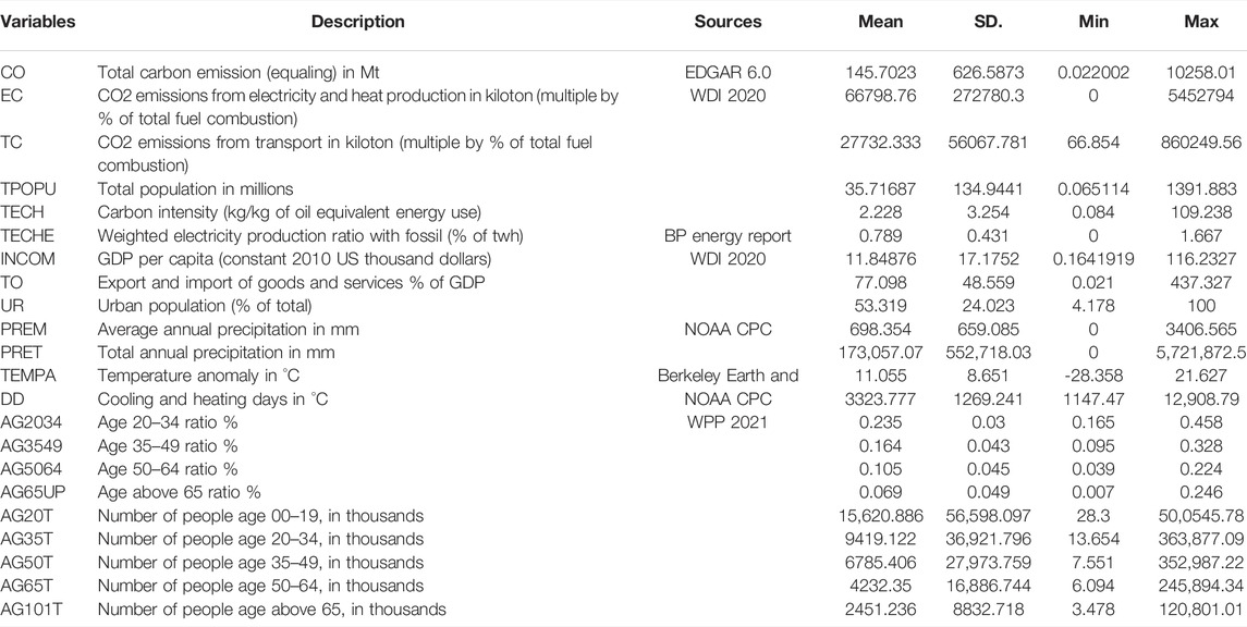
TABLE 2. Variable data sources and descriptive statistics.

4 Empirical Results

Considering the possible heterogeneity slope and cross-sectional correlation in panel data with long T and large N, we applied the wild cluster method and SURE model for the main regression, the threshold effect model to test for carbon peaking in each country under the EKC hypothesis; the robustness test is completed with changing indicators, adopting the panel mean group method and heterogeneity analysis with country classified by geographical region and climate types.

4.1 Baseline Regression Results

Based on the model described in Section 2, the empirical tests are conducted with panel data in 150 countries and regions from 1979 to 2013 (time restricted by climate data). At the same time, we will make group comparisons based on transportation and electricity carbon emissions. The Hausman test results support fixed-effects models. Table 3 presents the results after eliminating heteroscedasticity using weighted robust standard errors. In addition, the wild cluster bootstrap standard errors method (Yan and Lin, 2020) proposed in Cameron, Cameron et al. (2008) was used for later estimations. It can be observed that the coefficients of different age groups followed an inverted U-shape for total and heat and electricity carbon emissions, while transport carbon emissions are more likely to decrease by age.

TABLE 3

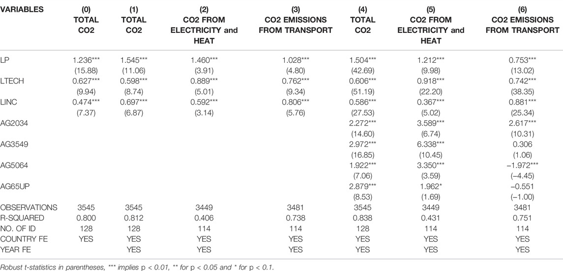
TABLE 3. Basic results of age structure and carbon emission

The carbon intensity indicator adopted here denotes how many standard units of carbon dioxide emissions are generated by one standard unit of energy consumption, which corresponds to the weighting average of the country’s energy mix (oil, coal, natural gas, clean energy, etc.) and energy efficiency or technology (some countries have higher oil utilization technology than others) in general. Suppose one country uses more clean energy than fossil, its carbon intensity (carbon emissions corresponding to energy consumption) will be smaller. At the same energy consumption level, countries that produce more carbon use more non-clean energy and inefficiently, so their technology level is considered to be lower (at least for energy use and carbon emissions) while the indicator gets larger. The positive coefficient of technology implies the relation that if a country adopts more renewable energy or improves energy efficiency, its carbon emission will decrease.

4.2 The Empirical Results of Age Structure and Climate Impacts on Carbon Emission

Columns (1)–(4) of Table 4 are the empirical result of the basic STIRPAT model. The results show that population, economic scale, and technology level are undoubtfully the main factors affecting carbon emissions. Generally, total population has the biggest impact on the total carbon emission. Technology level is very important for heat and electricity carbon emission, and the per capita income level is more important for transportation carbon emission. In column (4), the effect of population on carbon emission is separated into size effect and age structure effect. Population size effect is significantly positive with the elasticity coefficient is 1.078, very close to unity that carbon growth is in the same pace with population growth.

TABLE 4

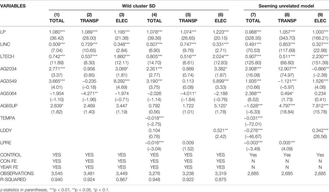
TABLE 4. Results of climate-extended STIRPAT with wild cluster bootstrap and SURE method

As for technology, carbon intensity also has a significantly positive effect, with a coefficient of 0.805, that is, for every 1% reduction in carbon intensity due to advances in energy utilization technology, total carbon emissions will decrease by 0.806%, so upgrading and promoting green technology is still an efficient and feasible means to achieve carbon emission reduction especially for the heat and electricity sector with coefficient 2.024. There is also significant positive correlation between economic level and total carbon emissions, with a coefficient of elasticity of 0.507, so overall the growth speed of carbon emission is slower than economic, which implies the promising future of carbon emission reduction and carbon neutrality. This can be explained by the fact that countries with higher levels of economic development pay more attention to environmental protection with the more advanced the technology of energy saving and emission reduction, but the total amount of energy consumption is still huge, so generally the efforts can only slow down the inevitable, the increase in per capita GDP still leads to total carbon emission increase. Our result is aligned with various previous studies (Poumanyvong and Kaneko, 2010; Zhukov et al., 2014; Shahbaz et al., 2017, Xu and Lin, 2015b, Liu and Bae, 2018).

4.2.1 Age Structure Impact on Carbon Emission

For total carbon emissions, the results of wild cluster bootstrap in column (4) shows that the age carbon emission coefficient of the population conforms to the inverted U-shape with uplift tail, notice each coefficient here stands for age-group specified deviation from the average impact of the total amount, for example, the carbon elasticity of the population aged 20–34 is 2.351% higher than the average carbon emission elasticity of the whole population, so every percentage change in 20–34 population ratio would lead to 2.351% change in total carbon emissions accordingly. Generally, column (4)–(6) of Table 4 shows that for the total carbon emission, the influence pattern of age structure conforms to the hypothesis H1. The consumption elasticity increases the start from the age of 20 (+2.351), reaches its peak value of carbon consumption at the age of 35–49 (+3.190), and decreases to lower than the average (−2.026) at the age of 50–64. After the age of 65, the carbon consumption starts to increase (+0.792) compared with the previous stage, and the inverted U-shaped curve begins to form an uplift tail. In terms of overall patterns, SURE and wild cluster bootstrap are basically showing the same results, increasing at first and then decreasing, and at last rising at the tail. The difference lies in the age of the peak carbon consumption, which may need further investigation into sub samples and more age groups. It can also be seen from variation of the coefficient in the transport sector that the pattern may exist though not at high significance level, the assumption H1 might still hold (see Section 4.4), the carbon emission decreases more (−4.011) after middle age, while the results of SUR show that the age peak on traffic carbon emission may be earlier than expected, closer to 35, decrease afterward, and then rise again after middle-age.

Both SURE and wild cluster bootstrap results indicate that the age peak of heat and electricity carbon emission is between 35 and 49. The difference lies in the increase and decrease range of the previous and latter age groups, sharper or milder in curve, which also confirms the H1 assumption. It is worth noting that the deviation of carbon consumption from people over 65 exceeds the previous peak value of young adults in both results, namely the tail is higher than the hump. For this strong uplifting tail phenomena, we have tests for Hypothesis 2 and found the explanation: the temperature regulation demand caused by the decline of physical adaptability along with age.

4.2.2 Cross-Effects of Population Aging and Degree-Days

From the above results, we find that aging does not slow down carbon emissions as expected, and the results of sub-sectors also suggest the existence of heterogeneity, from the real-life circumstance it can be observed that older people have more cooling and heating energy demand due to their body’s reduced environmental adaptability, which explains to some extent the rise in carbon emissions in the older age group. To verify the existence of this mechanism, the World Bank’s Ageing society criteria is used to set the country-specific dummy variable $ol{d}_{it}$ , and put its interaction term with degree-days into the equation. Results are presented in Table 5. From it we can see that the coefficient of the cross term $DegreeDays\times old$ is significantly positive, corroborating our Hypothesis 2 above. So, it proved that the uplifted tail of the inverted U-shaped carbon consumption pattern in the heat and electricity sector is indeed caused by the environmental temperature regulation demand of the elderly population for their declined physical adaptability. Despite the reduction of activities, the elderly need to keep their body comfortable, so as to consume more energy thus produces more carbon emissions.

TABLE 5

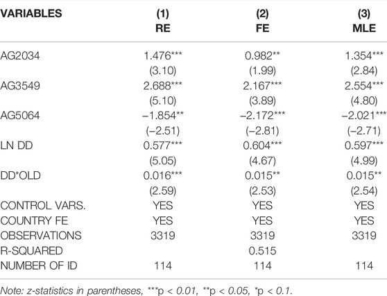
TABLE 5. The interaction effects of degree-days and population aging on electricity carbon emission

4.2.3 Climate Impact on Carbon Emission

As for the climate indicators, columns (4) and (7) of Table 4 show temperature anomalies have significant negative impacts on the total carbon emission, for every 1° rise in abnormal temperature, the global climate cooperation will be promoted and thus reduce the total carbon emission (in mt) by 1.8–3.1%. Note that the carbon emission decline and TA change here are the average values of long-term changes, the actual impact may be greater, which is in line with Assumption H3.

Columns (4) and (5) of Table 4 present that average annual precipitation (measured in mm) also has significant negative influence on total carbon emission (−0.003 to −0.016) and columns (7) and (8) show positive effect on transport sector (0.005–0.009), consistent with Assumption H4. For every 1% increase in precipitation annual mean (unit mm), the total carbon emission (in mt) will be down by 0.003–0.016% due to the overall effect by carbon sink of water and plants after canceled out by traffic jam effects; and the transport carbon emission (in mt) will be increased by 0.005–0.009% as the traffic congestion caused by bad weather conditions.

DD has the greatest impact among others, when annual DD increases by 1%, the change of total carbon emissions will be – 0.276–0.104% as in column (4) and (6), Assumption H5 is proved. This impact of DD is relatively large, especially in the heat and electricity sector from column (7) and (9), that for every 1% change in DD, the carbon emission will be increased by about 0.34–0.52%, that is stronger influence than the impact of per capita income growth on carbon, which reminds us that the improvement of building insulation technology is very necessary for carbon reduction.

4.3 Test of the Income and Technology Threshold on Carbon Emission

Table 5 reports the test results with carbon emission intensity and per capita income as the threshold. It can be seen that when per capita GDP and carbon emission intensity are used as the threshold variables, the corresponding F value passed the one-threshold and two-threshold models, and both were within 1% (error) Level passed the significance test. The significance level of the single threshold for per capita GDP is higher than the double threshold and the triple threshold. Therefore, we choose the single threshold for income, similar for carbon emission intensity. Under the single threshold hypothesis test, the logarithmic per capita GDP threshold value is 8.1, which is approximately $3,581.7257 USD per year, and according to the World Bank income category the transition value is near the low middle income dividing line, it also fits the heterogeneous results in Table 6. The carbon emission intensity threshold is 0.6026, which is 1.8269 kg/kg oil equivalent.

TABLE 6

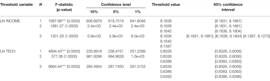
TABLE 6. Threshold tests and confidence intervals for GDP per capita and carbon intensity

These results confirm our previous results on the impact of demographic structure, but reveal that countries in different income status did have different pace in their carbon reduction along aging, thus calling for international cooperation in technology innovation on carbon reduction. Judging by the income thresholds, 97 out of 150 sample countries reached their peak carbon emissions before 2013 (Table 7).

TABLE 7

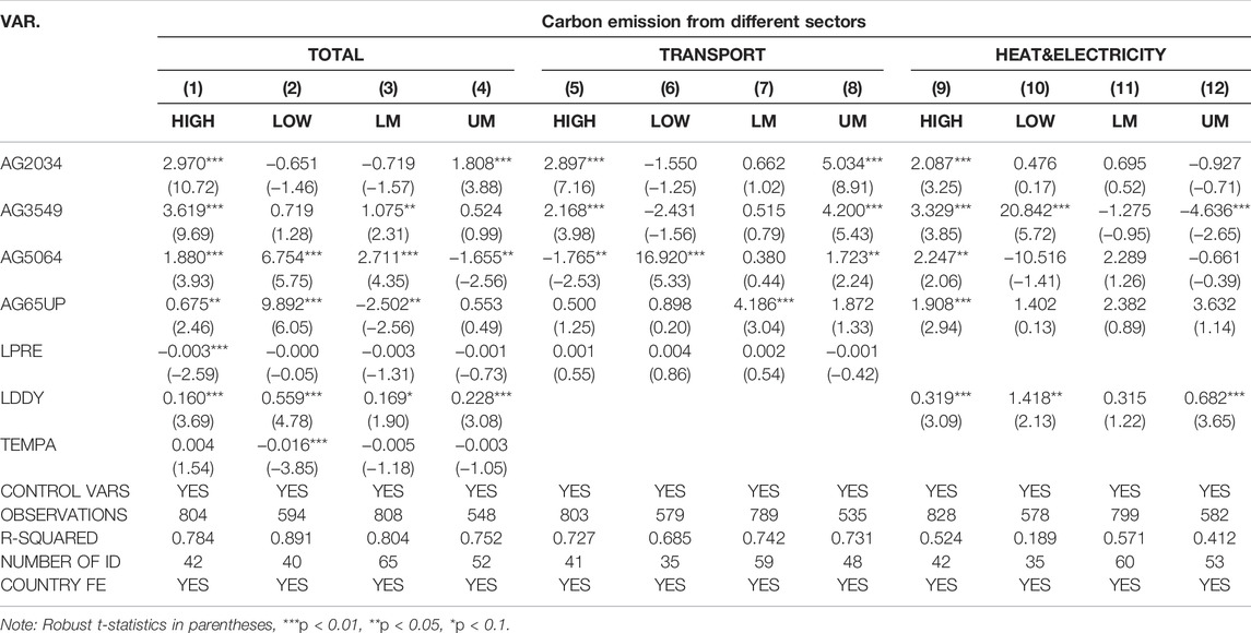
TABLE 7. Sample group divided by World Bank income level standard

To support this inverted U-shaped relationship regarding carbon emissions-income, we grouped the sample of countries according to the World Bank classification criteria (June 2019), noting that the criteria changed throughout the sample period, as each year the World Bank revises the classification of world economies based on the previous year’s GNI per capita, the standard value for the classification criteria are also increasing due to inflation. For the current 2020 fiscal year, using the World Bank Atlas method, low-income economies are defined as those with the GNI per capita of $1,025 or less in 2018; lower middle-income economies are those with the GNI per capita between $1,026 and $3,995; upper middle-income economies are those with the GNI per capita between $3,996 and $12,375; high-income economies are those with the GNI per capita of $12,376 or more.

The results of the income threshold test show that the turning point is between lower middle-income to upper middle-income, so it would be expected that the low-income and high-income groups would show different results, and Table 7 presents the results. Here we can notice that the high-income and low-income subgroups do behave differently in terms of carbon emissions. The results are also consistent with previous expectations too, with carbon emission coefficients for age fits the inverted U-shaped trend in high-income and lower-middle-income countries, while carbon emissions in upper-middle-income countries in transition presenting the pattern of fall and then rise with age, with significant upward tail in low-income countries, this phenomenon we consider related to the fact that life expectancy does not even reach 65 years in most low-income countries, due to factors such as lacking proper health care and war. Their carbon consumption habits might be more related to emergencies rather than the full-scale life cycle pattern.

4.4 Robustness Check

4.4.1 Changing the Demographic and Technology Indicator

If the percentage of the population in each age group is replaced with the absolute number, the conditions for the transformation of the logarithmic term into an additive relationship may not be met, but it is still possible to observe the trend through the sign of the grouping coefficients, as shown in Supplementary Table S3, where the coefficients show a strong inverted U-shaped trend, the hump pattern of carbon consumption along the age growing is very clear in all three carbon emission sectors.

What’s more, the sharp increase in carbon consumption in the population over 65 is interesting phenomenon, especially compared with the effect of people between 51 and 64 that turns negative, i.e., people in this age group show less carbon consumption compared to the whole life cycle average. This may be the result of that the older population, due to reduced physical adaptability, generate more need for cooling and heating and may also be less able to undertake the energy-efficient modes of travel such as walking and cycling. The impact of other climate factors is consistent with the previous assumptions and results.

If we use the weighted electricity production ratio by fossil source (with the IPCC carbon emission factors) as the indicator for carbon technology level to check for robustness, the regression results with the new technology indicators are shown in Supplementary Table S4. We can see the inverted U-shape of age carbon consumption pattern still exists, in total carbon emissions, the age-carbon emission elasticity reaches its maximum at the ages between 35–49, and in heat and electricity carbon emissions, the pattern is the same, the carbon emission elasticity of age above 65 is greater than that cohort between 50 and 64, while this tail-up change does not occur in transport carbon emissions, and as we mentioned in the previous analysis, this tail-up patterning in heat production and electricity carbon emissions is caused by the reduced environmental resilience of the elderly population.

Whereas the effect of this technology indicator on transport carbon emissions is not significant, as carbon technology for electricity is indeed not directly correlated with carbon technology for transport, in contrast to the total energy carbon intensity indicator shown in the main regression, which may be more representative of the level of carbon technology at the national economic level.

As for climate indicators, TA’s negative effects on total carbon emission is in accordance with our assumption and previous results as well as DD and PRE, and for DD in heat and electricity carbon sector there may exist the multicollinearity problem that leads to the insignificance, though sign of coefficients are fitted with assumption. The negative effect of precipitation on carbon emissions from traffic also confirms the assumption that congestion leads to an increase in carbon emissions per unit time.

4.4.2 Sub-sample by Continents and Climate Types

In line with the directions for further improvement mentioned in previous studies, it may be more reasonable to use climate type groupings to proxy the effects of climate heterogeneity than to examine patterns by grouping country samples by continent to which they belong. Though considering that the carbon emissions data used in the study were derived from EDGAR analysis of satellite imagery and the spatial spillover effects of greenhouse gases are normal, we have included regression results by regional grouping in this part for comparison. The following tables are arranged in the order of total carbon emissions, transport carbon emissions, and heat and electricity carbon emissions, all regressions are fixed effects based on the Hausman test.

Comparing the results in Supplementary Table S5 of the six continents, we find that there are two different patterns of carbon consumption by age. For the European and North American countries, as the population becomes more environmentally conscious with age, the average carbon consumption of the age group is lower compared to that of younger people, which is reflected in the decreasing carbon emission coefficient to the right side of the inverted U-shaped curve. In contrast, Asian, African, and South American countries still conform to the inverted U-shaped curve, except for the age range of carbon emissions peak. This confirms our results from the threshold effect test of the EKC hypothesis, which suggests that Europe and the US have already crossed the carbon peak and are moving toward a more sustainable consumption pattern.

Most of the results for climate factors are consistent with the hypothesis of the previous analysis, none of the PRE’s effects are significant, for the mechanisms of precipitation effects on carbon emissions are too complex. As we can see from Supplementary Table S6 results that in North America, Oceania, and South America, the effect of traffic congestion carbon emissions caused by precipitation is greater than the carbon sink effect, so the total carbon emissions effect of precipitation is still positive.

The effect of DD on carbon emissions is significantly positive in Africa, Asia, Europe, and North America, with the largest effect from Asian countries, which is also consistent with the results shown in Supplementary Table S7. The reason is that Asian countries are more severe in aging and elderly have a higher demand for heat and electricity; and the impact of TA is significantly negative in the Asian and African subgroups, indicating these countries have undertaken the strongest implementation of policies to reduce carbon emissions, and thus far, working effectively in the global climate cooperation.

For transport carbon emissions, similar findings of differential carbon emissions by age group hold, with the difference being the age cohort at which peak consumption is reached, which reflects the different household structures and travel habits caused by dominant cultural differences across continents. The positive effects by precipitation are significant in North America, Oceania, and South America, and reflect the fact that traffic fluidity in these regions is more likely to be affected by precipitation due to the combination of road design, vehicle composition, and guidance ability of transportation system factors. Moreover, for heat and electricity carbon emissions, similar findings of differential carbon emissions by age group hold, with the difference being the age cohort at which peak consumption is reached.

To examine the impact of climate heterogeneity, in addition to directly using climate indicators such as TA DD PRE in the regression, it can also be verified by comparing the regression results of Köppen group to explore whether there are differences in the impact of carbon emission determinations between different climate groups. As shown in Table 8, there are four climate groups (polar climate is ignored due to few samples), here ARD stands for arid, CONT stands for continental, TPR stands for temperate, and TROP stands for tropical. Detailed descriptions of the various climate types are in the Supplementary Appendix. It can be seen that differences in coefficients between climate types do exist.

TABLE 8

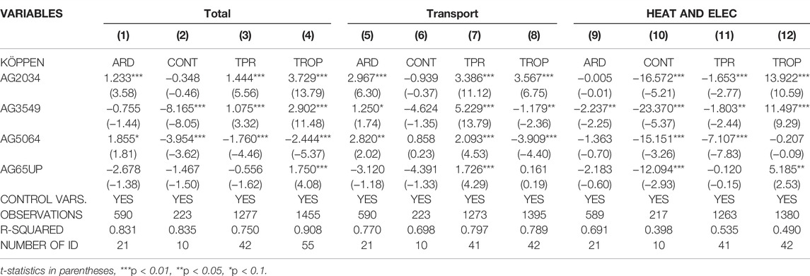
TABLE 8. Sample group divided by climate types with carbon emission

Taking the changes in total carbon emission as an example, in arid countries age-carbon elasticity began to rise from 20, decreased in the age of 35–49, and began to rise again in the age of 50–64. The carbon emission of the population aged 35–64 in the continental countries is lower than the average impact of population. Similar to the conclusion of the SUR results in Section 4.2, the age for peak carbon emission in tropical and temperate regions is close to 35 years old, and the lowest carbon emission is in age between 50 and 64, then increases after people turn 65 years old. Compared with the change dynamic in heat and electricity sector, it can be judged that this uplift tail is caused by the demand for temperature regulation, which verifies our hypothesis H5 for degree-days.

4.4.3 Results With the Mean Group Estimators

With Blackburne and Frank (2007) and Eberhardt (2012) as reference, considered the cross-nation datasets used in this study are large enough in time periods T and N that it is possible to estimate each nation separately to avoid the heterogeneous slopes in terms of big N (Pesaran and Smith, 1995; Shi, 2003; Pesaran et al., 1997; Pesaran et al., 1999; Phillips and Moon, 2000) and time series nonstationary problem raised by long T (Pesaran et al., 1997; Pesaran et al., 1999).

One solution is to use the mean-group estimator (Pesaran and Smith, 1995) or pooled mean-group estimator (Pesaran et al., 1997; Pesaran et al., 1999), the basic idea of mean-group is deal with everyone’s time series separately and to get the arithmetic average of coefficients as the results. With the MG estimator, intercepts slope and error variances are all allowed to differ. This study followed the recent work by Pesaran et al. (1997), Pesaran et al. (1999) and used the PMG estimator which allows intercepts, short-run slopes, and error variances to differ while the long-run coefficients are the same across groups, basically utilizing the advantage of both pooling and averaging. The results are shown in Supplementary Table S8.

The inverted U-shaped pattern of age coefficient still holds for total carbon emission, transport carbon emission, and heat and electricity carbon emission. In addition, for climate factors, the negative impact of temperature anomaly, the negative impact of precipitation, and the positive impact of degree-days on total carbon emission are consistent with our previous analysis and results, and degree days also has great impact on heat and electricity carbon emission, which should be paid attention to.

5 Conclusion and Policy Implications

5.1 Conclusion

This study confirms the different effects of age group proportion on carbon emission, that is, the inverted U-shaped relation indicates young people consume and generate carbon along with their age growth to the periods when they have family and offspring, as children grow up, the emission reached the peak. Then emission decreases as offspring become older enough to leave home. The consumption goes down as people retire and spouses pass away. The right side of the curve is not lower than the left side as older people also generate more carbon due to the narrowed preferable thermal range as their body gets weak, which fits the existing findings with micro-level data on household energy consumption pattern. So, the phenomenon demonstrated that aggregate data also indicate the same trend the household consumption pattern validated.

Specifically, the more people between 20 and 34 and above 50 were, the less carbon emission there will be, people in their prime of life carry the peak influence effect for carbon emission. The percentage of the population aged 35–49 has the most significant positive influence on total carbon emissions, followed by age group 20–34, and after the age of 50 the influence begins to turn with a negative trend, the percentage of the population aged 50–64 has little influence on total carbon emissions (maybe the effects of differences within the group cancel each other out). In contrast, the percentage of older people (above 65 years old) has a significantly negative influence on transport carbon emissions. This result is acceptable considering that the population aged 20–50 has more abundant wealth, the largest consumption expenditure in all categories, and the largest number of family members and is consistent with the inverted U-shaped relation findings mentioned in the theoretical parts.

For climate variables, the impact of degree-days on electricity and total carbon emissions is significantly positive, and the coefficient is relatively large. In the cross-examination with the aging degree, we found that the coefficient is also positive, suggesting that the aging population’s weaker environmental tolerance makes them demand more by cooling and heating, thus accelerating the growth of electricity carbon emissions.

5.2 Policy Implications

5.2.1 Global Cooperation Still Needed to Reduce Carbon Emissions

The role of global climate cooperation is still important, countries at different stages of development should plan a reasonable path to reach the carbon peak and reduce carbon emissions according to both international requirements and its capability, while pursuing a relatively fair distribution of carbon emission reduction responsibilities. The realities of developing countries should be taken into account when negotiating. For those countries that are far away from the carbon transition, the priority should still be promoting the economic development, then they were able to adopt energy-saving technologies and grasp the overall pace of carbon reduction; while those developed countries should act as the carbon reduction role models, providing institutions, policies, development models, and technologies for latecomers to learn from.

Developed countries should also continue to invest in low carbon technology innovations, raise the overall international level of carbon technology, lower the threshold for learning low carbon technology, and pull up the level of other developing countries by technology spillover; developing countries should strive to learn to catch up with the level of advanced technology, and develop and implement low carbon technology by upgrading routes according to the strengths and weaknesses of their industries.

As we can see the transportation sector and heat and electric sector are major carbon-emitting industries, there still is some room to improve the efficiency, it is a good start to replace fuel vehicles with more electric vehicles, another attempt should be using more renewable sources in power generation, countries with different energy resource endowment should start cooperating with neighboring countries to control and replace the proportion of thermal and coal power; and it should also be noted that the stability of the power system cannot be ignore as the need to regulate the ambient temperature increased dramatically under extreme weather. As the integration of multiple energy sources being the common trend, new scientific methods are also needed to identify systematic solutions for organizing clusters of energy hubs according to demands (Chen et al., 2018).

5.2.2 Insulation Projects and More Energy Efficient Buildings

As we can see from the empirical results, among all influential factors, HDD/CDD explains a lot for the carbon emission, which is intuitive and fits our observations in life. So, the question becomes “how to make our buildings green” in a sense that not only requires the materials for a building process be environmentally friendly, but also the whole life cycle emits less dangerous chemicals.

The concept is similar to [energy efficient buildings] code, essential is how to make our buildings more livable and maintain a particular temperature moderation function under the natural solar energy system so that the energy demand for the air conditioner will naturally decrease, and thus our carbon emission. While being less discussed by economic studies, the [insulation] or its relationship with GHG emission has been thoroughly discussed in engineering fields. As for the protocol of energy-efficient buildings, the Trias Energetica concept is proposed with aspects: bioclimatic buildings - shape and orientation of buildings, solar protection, and passive solar systems. Among all the other factors, insulation of the envelope is undoubtfully the first step to improve energy efficiency. Taking the renovation work of old buildings as an example, we could hardly adjust the building orientation and structure once the construction finished; insulation material upgrade seems to be the only amendment. Also, it has been well discussed and proved that thermal insulation should be ranked at the top of the most effective investments for energy saving. A relatively small carbon footprint’ investment’ in thermal insulation materials yields significant savings in the operational time of a building because it saves energy in each heating season (Alam et al.,2011; Monahan and Powell, 2011; Singh and Limbachiya, 2011; Mazor et al., 2011; Jeanjean et al., 2013; Takano et al., 2014a; Stazi et al.,2015; Kunič, 2017).

In addition, different regions have different climates types–long winter or long summer, residents have different cooling and heating needs, so governments should take into account their own climatic features in updating the building standards, requiring the cradle-to-site assessment of the building using the Life Cycle Assessment (LCA) framework as an option (Takano et al., 2014b; Stazi et al., 2018; Strza\lkowski and Garbalińska, 2018; Pajek et al., 2017; Rodrigues et al., 2019). In addition to the improved design standards, retrofitting older houses is equally essential for reducing emissions as Li and Densley Tingley (2021) present, the cumulative carbon reduction potential from 2021 to 2050 is predicted to be 268 MtCO2, with all Victorian houses in Britain retrofitted. It is feasible for the government to initiate some infrastructure projects or housing renovation schemes to provide some financial subsidies for insulation upgrades, which is the cost-effective option in terms of the green economics. With the global outlook on carbon reduction, the revolution is coming for building contractors, building material manufacturers, and distributors. Coping with that, engineers need to change the design philosophy toward energy-efficient, and material suppliers should abandon polluting and inefficient materials and turn to green materials; for residents, it is important to understand the knowledge and choose ambient temperature devices with higher carbon efficiency.

Data Availability Statement

Information about the data processing methods, which involving some GIS operations, can be obtained from the authors upon request. The climate data is temporarily inaccessible in the public source to anonymously download, it will be made public once subsequent projection research is completed, any further inquiries can be sent to amospade@hotmail.com.

Author Contributions

WL and DX contributed to conception and design of the study. Wan Liu collected and processed the data with STATA and ARCGIS, performed the empirical analysis, wrote the drafts of the manuscripts, responded to the reviewers and editing the language and formats. Zhechong Luo validated the empirical method, polished the language of manuscripts and responses. De Xiao provided funding and suggestions to the framework of the study. All authors contributed to manuscript revision, read, and approved the submitted version.

Funding

This research was funded by the Key Projects (No. 19AJL016) of National Social Science Foundation, and the Foundation of the Ministry of Education of China for Outstanding Young Teachers in University (Grant No. 19YJC790152).

Conflict of Interest

The authors declare that the research was conducted in the absence of any commercial or financial relationships that could be construed as a potential conflict of interest.

Publisher’s Note

All claims expressed in this article are solely those of the authors and do not necessarily represent those of their affiliated organizations, or those of the publisher, the editors, and the reviewers. Any product that may be evaluated in this article, or claim that may be made by its manufacturer, is not guaranteed or endorsed by the publisher.

Acknowledgments

This research was selected as the conference paper of ICEF 2021, Xiamen. We appreciate the organizing works from China Energy Finance Network, Xiamen University, and Chinese Society of Optimization, Overall Planning and Economical Mathematics, and thank the session chair and audiences for helpful discussion and advice. Special Thanks to Prof. Syed Jawad Hussain Shahzad for his patient guidance on article framing and writing, and his kindly suggestions on the feasibility of the empirical methods.

Supplementary Material

The Supplementary Material for this article can be found online at: https://www.frontiersin.org/articles/10.3389/fenvs.2021.719168/full#supplementary-material

Footnotes

¹IEA, Global energy-related CO₂ emissions by sector, IEA, Paris https://www.iea.org/data-and-statistics/charts/global-energy-related-co2-emissions-by-sector.

²Thanks to the suggestion by Prof. Shahzad.

References

Ahmed, Z., Zafar, M. W., and Ali, S. D. (2020). Linking Urbanization, Human Capital, and the Ecological Footprint in G7 Countries: An Empirical Analysis. Sust. Cities Soc. 55, 102064. doi:10.1016/j.scs.2020.102064

CrossRef Full Text | Google Scholar

Alam, M., Singh, H., and Limbachiya, M. C. (2011). Vacuum Insulation Panels (VIPs) for Building Construction Industry - A Review of the Contemporary Developments and Future Directions. Appl. Energ. 88, 3592–3602. doi:10.1016/j.apenergy.2011.04.040

CrossRef Full Text | Google Scholar

Balaras, C. A., Droutsa, K., Dascalaki, E., and Kontoyiannidis, S. (2005). Heating Energy Consumption and Resulting Environmental Impact of European Apartment Buildings. Energy and Buildings 37 (5), 429–442. Available at: https://www.sciencedirect.com/science/article/pii/S0378778804002464. doi:10.1016/j.enbuild.2004.08.003

CrossRef Full Text | Google Scholar

Belaïd, F. (2016). Understanding the Spectrum of Domestic Energy Consumption: Empirical Evidence from France. Energy Policy 92, 220–233. Available at: https://www.sciencedirect.com/science/article/pii/S030142151630057X.

Google Scholar

Bhattacharjee, , Suchismita, , and Reichard, G. (2012). Socio-Economic Factors Affecting Individual Household Energy Consumption: A Systematic Review. Am. Soc. Mech. Eng. Digital Collect. 891–901. doi:10.1115/ES2011-54615

CrossRef Full Text | Google Scholar

Biørn, E. (2004). Regression Systems for Unbalanced Panel Data: A Stepwise Maximum Likelihood Procedure. J. Econom. 122 (2), 281–291. doi:10.1016/j.jeconom.2003.10.023

CrossRef Full Text | Google Scholar

Blackburne, E. F., and Frank., M. W. (2007). Estimation of Nonstationary Heterogeneous Panels. Stata J. 7, 197–208. doi:10.1177/1536867X0700700204

CrossRef Full Text | Google Scholar

BP (2018). 2015-2017 Data of the BP Statistical Review of World Energy.

Google Scholar

Carlsson-Kanyama, A., and Lindén, A.-L. (1999). Travel Patterns and Environmental Effects Now and in the Future:. Ecol. Econ. 30 (3), 405–417. Available at: https://www.sciencedirect.com/science/article/pii/S0921800999000063. doi:10.1016/s0921-8009(99)00006-3

CrossRef Full Text | Google Scholar

Cameron, A. C., Jonah, B. G., and Douglas, L. M. (2008). Bootstrap-Based Improvements for Inference with Clustered Errors. Rev. Econ. Statist. 90 (3), 414–427. doi:10.1162/rest.90.3.414

CrossRef Full Text | Google Scholar

Changnon, S. A. (1996). Effects of Summer Precipitation on Urban Transportation. Climatic Change 32, 481–494. doi:10.1007/BF00140357

CrossRef Full Text | Google Scholar

Chen, Y., Wei, W., Liu, F., Wu, Q., and Mei, S. (2018). Analyzing and Validating the Economic Efficiency of Managing a Cluster of Energy Hubs in Multi-Carrier Energy Systems. Appl. Energ. 230, 403–416. doi:10.1016/j.apenergy.2018.08.112

CrossRef Full Text | Google Scholar

Chen, J., Xiaohong, W., and Koen, S. (2013). A Statistical Analysis of a Residential Energy Consumption Survey Study in Hangzhou, China. Energy Build. 66, 193–202. doi:10.1016/j.enbuild.2013.07.045

CrossRef Full Text | Google Scholar

Cole, M. A., Rayner, A. J., and Bates, J. M. (1997). The Environmental Kuznets Curve: An Empirical Analysis. Envir. Dev. Econ. 2, 401–416. doi:10.1017/s1355770x97000211

CrossRef Full Text | Google Scholar

Crippa, M., Oreggioni, G., Guizzardi, D., Muntean, M., Schaaf, E., Lo Vullo, E., et al. (2019). Fossil CO2 and GHG Emissions of All World Countries - 2019 ReportEUR 29849 EN. Luxembourg: Publications Office of the European Union. doi:10.2760/687800.JRC117610

CrossRef Full Text | Google Scholar

Dietz, T., and Rosa, E. A. (1997). Effects of Population and Affluence on CO2 Emissions. Proc. Natl. Acad. Sci. 941, 175–179. doi:10.1073/pnas.94.1.175

CrossRef Full Text | Google Scholar

Eberhardt, M. (2012). Estimating Panel Time-Series Models with Heterogeneous Slopes. Stata J. 12, 61–71. doi:10.1177/1536867X1201200105

CrossRef Full Text | Google Scholar

Ehrlich, P. R., and Holdren, J. P. (1971). Impact of Population Growth. Science 171, 1212–1217. doi:10.1126/science.171.3977.1212

PubMed Abstract | CrossRef Full Text | Google Scholar

Engelman, R. (1994). Stabilizing the Atmosphere: Population, Consumption and Greenhouse Gases.

Google Scholar

European Commission (2021). “Joint Research Centre (EC-JRC)/Netherlands Environmental Assessment Agency (PBL),” in Emissions Database for Global Atmospheric Research (EDGAR), Release EDGAR v6.0_GHG (1970 - 2018) of.

Google Scholar

Fan, Y., Liu, L.-C., Wu, G., and Wei, Y.-M. (2006). Analyzing Impact Factors of CO2 Emissions Using the STIRPAT Model. Environ. Impact Assess. Rev. 26 (4), 377–395. doi:10.1016/j.eiar.2005.11.007

CrossRef Full Text | Google Scholar

Fang, Y., Michalak, A. M., Schwalm, C. R., Huntzinger, D. N., Berry, J. A., Ciais, P., et al. (2017). Global Land Carbon Sink Response to Temperature and Precipitation Varies with ENSO Phase. Environ. Res. Lett. 12, 064007. doi:10.1088/1748-9326/aa6e8e

CrossRef Full Text | Google Scholar

Fritzsche, D. J. (1981). An Analysis of Energy Consumption Patterns by Stage of Family Life Cycle. J. Marketing Res. 18 (2), 227–232. doi:10.1177/00222437810180020910.2307/3150956

CrossRef Full Text | Google Scholar

Gemechu Legesse, T., Dong, G., Jiang, S., Chen, J., Dong, X., Alemu Daba, N., et al. (2021). Small Precipitation Events Enhance the Eurasian Grassland Carbon Sink. Ecol. Indicators 131, 108242. doi:10.1016/j.ecolind.2021.108242

CrossRef Full Text | Google Scholar

Ghazali, A., and Ali, G. (2019). Investigation of Key Contributors of CO2 Emissions in Extended STIRPAT Model for Newly Industrialized Countries: A Dynamic Common Correlated Estimator (DCCE) Approach. Energ. Rep. 5, 242–252. doi:10.1016/j.egyr.2019.02.006

CrossRef Full Text | Google Scholar

Gleason, K. L., Lawrimore, J. H., Levinson, D. H., Karl, T. R., and Karoly, D. J. (2008). A Revised U.S. Climate Extremes Index. J. Clim. 21, 2124–2137. doi:10.1175/2007jcli1883.1

CrossRef Full Text | Google Scholar

Gokhale, S., and Pandian, S. (2007). A Semi-empirical Box Modeling Approach for Predicting the Carbon Monoxide Concentrations at an Urban Traffic Intersection. Atmos. Environ. 41, 367940–367950. doi:10.1016/j.atmosenv.2007.06.065

CrossRef Full Text | Google Scholar

Hansen, B. E. (1999). Threshold Effects in Non-dynamic Panels: Estimation, Testing, and Inference. J. Econom. 93, 345–368. doi:10.1016/s0304-4076(99)00025-1

CrossRef Full Text | Google Scholar

Hao, Y., Chen, H., Wei, Y.-M., and Li, Y.-M. (2016). The Influence of Climate Change on CO 2 (Carbon Dioxide) Emissions: An Empirical Estimation Based on Chinese Provincial Panel Data. J. Clean. Prod. 131, 667–677. doi:10.1016/j.jclepro.2016.04.117

CrossRef Full Text | Google Scholar

Hasselmann, K. (1976). Stochastic Climate Models Part I. Theory. Tellus 28, 473–485. doi:10.3402/tellusa.v28i6.11316

CrossRef Full Text | Google Scholar

Hranac, R., Sterzin, E. D., Krechmer, D., Rakha, H., and Farzaneh, M.United States. Federal Highway Administration (2006). Road Weather Management Program. “Empirical Studies on Traffic Flow in Inclement Weather. Available at: https://rosap.ntl.bts.gov/view/dot/42251.

Google Scholar

Jeanjean, A., Olives, R., and Py, X. (2013). Selection Criteria of Thermal Mass Materials for Low-Energy Building Construction Applied to Conventional and Alternative Materials. Energy and Buildings 63, 36–48. doi:10.1016/j.enbuild.2013.03.047

CrossRef Full Text | Google Scholar

Ji, X., and Chen, B. (2017). Assessing the Energy-Saving Effect of Urbanization in China Based on Stochastic Impacts by Regression on Population, Affluence and Technology (STIRPAT) Model. J. Clean. Prod. 163, S306–S314. doi:10.1016/j.jclepro.2015.12.002

CrossRef Full Text | Google Scholar

Kais, S., and Sami, H. (2016). An Econometric Study of the Impact of Economic Growth and Energy Use on Carbon Emissions: Panel Data Evidence from Fifty Eight Countries. Renew. Sust. Energ. Rev. 59, 1101–1110. doi:10.1016/j.rser.2016.01.054

CrossRef Full Text | Google Scholar

Kim, J., Lim, H., and Jo, H.-H. (2020). Do Aging and Low Fertility Reduce Carbon Emissions in Korea? Evidence from IPAT Augmented EKC Analysis. Ijerph 17, 2972. doi:10.3390/ijerph17082972

PubMed Abstract | CrossRef Full Text | Google Scholar

Kunič, R. (2017). Carbon Footprint of Thermal Insulation Materials in Building Envelopes. Energy Efficiency 10, 1511–1528. doi:10.1007/s12053-017-9536-1

CrossRef Full Text | Google Scholar

Leahy, E., and Lyons, S. (2010). Energy Use and Appliance Ownership in Ireland. Energy Policy 38, 4265–4279. doi:10.1016/j.enpol.2010.03.056

CrossRef Full Text | Google Scholar

Li, H., Mu, H., Zhang, M., and Li, N. (2011). Analysis on Influence Factors of China's CO2 Emissions Based on Path-STIRPAT Model. Energy Policy 39 (11), 6906–6911. doi:10.1016/j.enpol.2011.08.056

CrossRef Full Text | Google Scholar

Li, X., and Densley Tingley, D. (2021). Solid Wall Insulation of the Victorian House Stock in England: A Whole Life Carbon Perspective. Building Environ. 191, 107595. doi:10.1016/j.buildenv.2021.107595

CrossRef Full Text | Google Scholar

Li, X., Zhou, Y., Zhao, M., and Zhao, X. (2020). A Harmonized Global Nighttime Light Dataset 1992-2018. Sci. Data 7, 168. doi:10.1038/s41597-020-0510-y

PubMed Abstract | CrossRef Full Text | Google Scholar

Liddle, B. (2014). Impact of Population, Age Structure, and Urbanization on Carbon Emissions/Energy Consumption: Evidence from Macro-Level, Cross-Country Analyses. Popul. Environ. 35, 286–304. doi:10.1007/s11111-013-0198-4

CrossRef Full Text | Google Scholar

Liddle, B., and Lung, S. (2010). Age-Structure, Urbanization, and Climate Change in Developed Countries: Revisiting STIRPAT for Disaggregated Population and Consumption-Related Environmental Impacts. Popul. Environ. 31, 317–343. doi:10.1007/s11111-010-0101-5

CrossRef Full Text | Google Scholar

Liddle, B. (2015). What Are the Carbon Emissions Elasticities for Income and Population? Bridging STIRPAT and EKC via Robust Heterogeneous Panel Estimates. Glob. Environ. Change 31, 62–73. doi:10.1016/j.gloenvcha.2014.10.016

CrossRef Full Text | Google Scholar

Liu, X., and Bae, J. (2018). Urbanization and Industrialization Impact of CO₂ Emissions in China. J. Clean. Prod. 172, 178–186. doi:10.1016/j.jclepro.2017.10.156

CrossRef Full Text | Google Scholar

Lv, Y., Chen, W., and Cheng, J. (2019). Modelling Dynamic Impacts of Urbanization on Disaggregated Energy Consumption in China: A Spatial Durbin Modelling and Decomposition Approach. Energy Policy 133, 110841. doi:10.1016/j.enpol.2019.06.049

CrossRef Full Text | Google Scholar

Long, Y., Yoshikuni, Y., Jing, M., Dabo, G., Liming, Y., and Haoran, Z. (2019). Unequal Age-Based Household Emission and Its Monthly Variation Embodied in Energy Consumption – A Cases Study of Tokyo, Japan. Appl. Energy 247, 350–362. doi:10.1016/j.apenergy.2019.04.01

CrossRef Full Text | Google Scholar

Manabe, S., and Stouffer, R. J. (1980). Sensitivity of a Global Climate Model to an Increase of CO2concentration in the Atmosphere. J. Geophys. Res. 85, 5529–5554. doi:10.1029/JC085iC10p05529

CrossRef Full Text | Google Scholar

Mazor, M. H., MuttonRussell, J. D, David, . A. M., Russell, D. A. M., and Keoleian, G. A. (2011). Life Cycle Greenhouse Gas Emissions Reduction from Rigid Thermal Insulation Use in Buildings. Journal Ind. Ecology 15, 284–299. doi:10.1111/j.1530-9290.2010.00325.x(

CrossRef Full Text | Google Scholar

Meyerson, F. A. B. (1998). Population, Carbon Emmissions, and Global Warming: The Forgotten Relationship at Kyoto. Popul. Dev. Rev. 24, 115–130. doi:10.2307/2808124

CrossRef Full Text | Google Scholar

Mirasgedis, S. Y., Sarafidis, E., Georgopoulou, D. P., Lalas, M., Moschovits, F., Karagiannis, , et al. (2006). Models for Mid-Term Electricity Demand Forecasting Incorporating Weather Influences. Energy 31 (2), 208–227. doi:10.1016/j.energy.2005.02.016

CrossRef Full Text | Google Scholar

Monahan, J., and Powell, J. C. (2011). An Embodied Carbon and Energy Analysis of Modern Methods of Construction in Housing: A Case Study Using a Lifecycle Assessment Framework. Energy and Buildings 43, 179–188. doi:10.1016/j.enbuild.2010.09.005

CrossRef Full Text | Google Scholar

Muller, R. A., Curry, J., Groom, D., Jacobsen, R., Perlmutter, S., Rohde, R., et al. (2013). Decadal Variations in the Global Atmospheric Land Temperatures. J. Geophys. Res. Atmos. 118, 5280–5286. doi:10.1002/jgrd.50458

CrossRef Full Text | Google Scholar

Nemani, R., White, M., Thornton, P., Nishida, K., Reddy, S., Jenkins, J., et al. (2002). Recent Trends in Hydrologic Balance Have Enhanced the Terrestrial Carbon Sink in the United States. Geophys. Res. Lett. 29 (10), 106-1–106-4. doi:10.1029/2002GL014867

CrossRef Full Text | Google Scholar

Olivier, J., and Janssens-Maenhout, G. (2015). "Part III: Total Greenhouse Gas Mmissions," in CO2 Emissions from Fossil Fuel Combustion. Paris Cedex, France: International Energy Agency (OECD), 427–538.

Google Scholar

Pachauri, S. (2004). An Analysis of Cross-Sectional Variations in Total Household Energy Requirements in India Using Micro Survey Data. Energy Policy 32(15), 1723–1735. Available at: https://www.sciencedirect.com/science/article/pii/S0301421503001629.

CrossRef Full Text | Google Scholar

Pajek, L., Blaž, H., Roman, K., and Mitja, K. (2017). Improving Thermal Response of Lightweight Timber Building Envelopes during Cooling Season in Three European Locations. J. Clean. Prod. 156, 939–952. doi:10.1016/j.jclepro.2017.04.098

CrossRef Full Text | Google Scholar

Pardo, A., Vicente, M., and Enric, V. (2002). Temperature and Seasonality Influences on Spanish Electricity Load. Energy Econ. 24 (1), 55–70. doi:10.1016/S0140-9883(01)00082-2

CrossRef Full Text | Google Scholar

Pesaran, M. H., and Smith, R. (1995). Estimating Long-Run Relationships from Dynamic Heterogeneous Panels. J. Econ. 68 (1), 79–113. doi:10.1016/0304-4076(94)01644-F

CrossRef Full Text | Google Scholar

Pesaran, M. H., Shin, Y., and Smith, R. P. (1997). “Pooled Estimation of Long-Run Relationships in Dynamic Heterogeneous Panels. Cambridge Working Papers in Economics,” in Faculty of Economics. Cambridge, United Kingdom: University of Cambridge. https://ideas.repec.org/p/cam/camdae/9721.html

Google Scholar

Pesaran, M. H., Yongcheol, S., and Ron, P. S. (1999). Pooled Mean Group Estimation of Dynamic Heterogeneous Panels.” J. Am. Statist. Assoc. 94 (446), 621–634. doi:10.1080/01621459.1999.10474156

CrossRef Full Text | Google Scholar

Phillips, P. C. B., and Moon, H. R. (2000). Nonstationary Panel Data Analysis: An Overview of Some Recent Developments. Econ. Rev. 19 (3), 263–286. doi:10.1080/07474930008800473

CrossRef Full Text | Google Scholar

Pilli-Sihvola, K., Piia Aatola, M. O., and Heikki, T. (2010). Climate Change and Electricity Consumption—Witnessing Increasing or Decreasing Use and Costs? Energy Policy 38 (5), 2409–2419. doi:10.1016/j.enpol.2009.12.033

CrossRef Full Text | Google Scholar

Poumanyvong, P., and Kaneko, S. (2010). Does Urbanization lead to Less Energy Use and Lower CO2 Emissions? A Cross-Country Analysis. Ecol. Econ. 702, 434–444. doi:10.1016/j.ecolecon.2010.09.029

CrossRef Full Text | Google Scholar

Ripple, W. J., Wolf, C., Newsome, T. M., Gregg, J. W., Lenton, T. M., Palomo, I., et al. (2021). World Scientists' Warning of a Climate Emergency 2021. BioScience 71, 894–898. doi:10.1093/biosci/biab079

CrossRef Full Text | Google Scholar

Rohde, R., Muller, R A., et al. (2013a). A New Estimate of the Average Earth Surface Land Temperature Spanning 1753 to 2011. Geoinfor Geostat: An Overview 1, 1. doi:10.4172/gigs.1000101

CrossRef Full Text | Google Scholar

Rohde, R., Muller, R. A., Jacobsen, R., Perlmutter, S., Rosenfeld, A., Wurtele, R., et al. (2013b). Berkeley Earth Temperature Averaging Process. Geoinfor Geostat: An Overview 1, 2. doi:10.4172/gigs.100010310.4172/2327-4581.1000103

CrossRef Full Text | Google Scholar

Rodrigues, E., Marco, S. F., Adélio Rodrigues Gaspar, Á. G., and José, J. C. (2019). Thermal Transmittance Effect on Energy Consumption of Mediterranean Buildings with Different Thermal Mass. Appl. Energy 252, 113437. doi:10.1016/j.apenergy.2019.113437

CrossRef Full Text | Google Scholar

Salim, R., Rafiq, S., Shafiei, S., and Yao, Y. (2019). Does Urbanization Increase Pollutant Emission and Energy Intensity? Evidence from Some Asian Developing Economies. Appl. Econ. 51, 4008–4024. doi:10.1080/00036846.2019.1588947

CrossRef Full Text | Google Scholar

Shafiei, S., and Salim, R. A. (2014). Non-renewable and Renewable Energy Consumption and CO2 Emissions in OECD Countries: A Comparative Analysis. Energy Policy 66, 547–556. doi:10.1016/j.enpol.2013.10.064

CrossRef Full Text | Google Scholar

Shahbaz, M., Chaudhary, A. R., and Ozturk., I. (2017). Does Urbanization Cause Increasing Energy Demand in Pakistan? Empirical Evidence from STIRPAT Model. Energy 122, 83–93. doi:10.1016/j.energy.2017.01.080

CrossRef Full Text | Google Scholar

Sheng, P., and Guo, X. (2016). The Long-Run and Short-Run Impacts of Urbanization on Carbon Dioxide Emissions. Econ. Model. 53, 208–215. doi:10.1016/j.econmod.2015.12.006

CrossRef Full Text | Google Scholar

Shi, A. (2003). The Impact of Population Pressure on Global Carbon Dioxide Emissions, 1975-1996: Evidence from Pooled Cross-Country Data. Ecol. Econ. 441, 29–42. doi:10.1016/s0921-8009(02)00223-9

CrossRef Full Text | Google Scholar

Singh, A. M. H., and Limbachiya, M. C. (2011). Vacuum Insulation Panels (VIPs) for Building Construction Industry – A Review of the Contemporary Developments and Future Directions. Appl. Energy 88 (11), 3592–3602. doi:10.1016/j.apenergy.2011.04.040

CrossRef Full Text | Google Scholar

Sovacool, B. K., Noel, L., Kester, J., and Zarazua de Rubens, G. (2018). Reviewing Nordic Transport Challenges and Climate Policy Priorities: Expert Perceptions of Decarbonisation in Denmark, Finland, Iceland, Norway, Sweden. Energy 165, 532–542. doi:10.1016/j.energy.2018.09.110

CrossRef Full Text | Google Scholar

Stazi, F., Bonfigli, C., Tomassoni, E., Di Perna, C., and Munafò, P. (2015). The Effect of High Thermal Insulation on High Thermal Mass: Is the Dynamic Behaviour of Traditional Envelopes in Mediterranean Climates Still Possible. Energy and Buildings 88, 367–383. doi:10.1016/j.enbuild.2014.11.056

CrossRef Full Text | Google Scholar

Stazi, F., Ulpiani, G., Pergolini, M., and Di Perna, C. (2018). The Role of Areal Heat Capacity and Decrement Factor in Case of Hyper Insulated Buildings: An Experimental Study. Energy Build. 176, 310–324. doi:10.1016/j.enbuild.2018.07.034

CrossRef Full Text | Google Scholar

Stott, P. (2016). How Climate Change Affects Extreme Weather Events. Science 352, 1517–1518. doi:10.1126/science.aaf7271

CrossRef Full Text | Google Scholar

Strza\lkowski, J., and Garbalińska, H. (2018). Thermal Simulation of Building Performance with Different Loadbearing Materials. IOP Conf. Series. 415, 012014. doi:10.1088/1757-899X/415/1/012014

CrossRef Full Text | Google Scholar

Su, K., Wei, D.-z., and Lin, W.-x. (2020). Influencing Factors and Spatial Patterns of Energy-Related Carbon Emissions at the City-Scale in Fujian Province, Southeastern China. J. Clean. Prod. 244, 118840. doi:10.1016/j.jclepro.2019.118840

CrossRef Full Text | Google Scholar

Takano, A., Hughes, M., and Winter, S. (2014a). A Multidisciplinary Approach to Sustainable Building Material Selection: A Case Study in a Finnish Context. Building Environ. 82, 526–535. doi:10.1016/j.buildenv.2014.09.026

CrossRef Full Text | Google Scholar

Takano, A., Stefan, W., Mark, H., and Lauri, L. (2014b). Comparison of Life Cycle Assessment Databases: A Case Study on Building Assessment. Build. Environ. 79, 20–30. doi:10.1016/j.buildenv.2014.04.025

CrossRef Full Text | Google Scholar

Tarazkar, M. H., Dehbidi, N. K., Ozturk, I., and Al-mulali, U. (2020). The Impact of Age Structure on Carbon Emission in the Middle East: The Panel Autoregressive Distributed Lag Approach. Environ. Sci. Pollut. Res. 28, 33722–33734. doi:10.1007/s11356-020-08880-4

CrossRef Full Text | Google Scholar

Thom, H. C. S. (1952). Seasonal Degree-Day Statistics for the United States. Mon. Weather Rev. 80 (9), 143–147. doi:10.1175/1520-0493(1952)080%3C0143:SDSFTU%3E2.0.CO;2

CrossRef Full Text | Google Scholar

Vélez-Henao, J.-A., Font Vivanco, D., Hernández-Riveros, J.-A., and Jesús-Antonio Hernández-Riveros, (2019). Technological Change and the Rebound Effect in the STIRPAT Model: A Critical View. Energy Policy 129, 1372–1381. doi:10.1016/j.enpol.2019.03.044

CrossRef Full Text | Google Scholar

Vilhelmsson, B. (1988). “Befolkningen Resvanor I Ett tidsperpektiv.Livscykel Och Gerenationsaspekter Perioden 1978 – 1985,” in Time Perspectives on Travel Patterns in Sweden. Lifecycleand Generational Changes in the Access and Use of Transporta-Tion from 1978 to 1985 (Gothenburg, Sweden: Department of Human and Economic Geography. University of Gothenburg).

Google Scholar

Wang, S., Wu, W., Zhu, B., and Wei, Y. (2013). Examining the Impact Factors of Energy-Related CO2 Emissions Using the STIRPAT Model in Guangdong Province, China. Appl. Energ., 106, 65–71. doi:10.1016/j.apenergy.2013.01.036

CrossRef Full Text | Google Scholar

Wang, Q., and Zhang, F. (2021). The Effects of Trade Openness on Decoupling Carbon Emissions from Economic Growth - Evidence from 182 Countries. J. Clean. Prod. 279, 123838. doi:10.1016/j.jclepro.2020.123838

PubMed Abstract | CrossRef Full Text | Google Scholar

Wang, Z., Rasool, Y., Zhang, B., Ahmed, Z., and Wang, B. (2020). Dynamic Linkage Among Industrialisation, Urbanisation, and CO2 Emissions in APEC Realms: Evidence Based on DSUR Estimation. Struct. Change Econ. Dyn. 52, 382–389. doi:10.1016/j.strueco.2019.12.001

CrossRef Full Text | Google Scholar

Wickham, C., Rohde, R., Muller, R. A., Wurtele, J., Curry, J., Groom, D., et al. (2013). Influence of Urban Heating on the Global Temperature Land Average Using Rural Sites Identified from MODIS Classifications. Geoinfor Geostat: An Overview 1, 2. doi:10.4172/gigs.100010410.4172/2327-4581.1000104

CrossRef Full Text | Google Scholar

Xu, B., and Lin, B. (2015b). How Industrialization and Urbanization Process Impacts on CO₂ Emissions in China: Evidence from Nonparametric Additive Regression Models. Energy Econ. 48, 188–202. doi:10.1016/j.eneco.2015.01.005

CrossRef Full Text | Google Scholar

Yan, Z., and Lin, B. (2020). WCBREGRESS: Stata Module to Estimate a Linear Regression Model with Clustered Errors Using the Wild Cluster Bootstrap Standard Errors. Statistical Software Components. Boston: Boston College Department of Economics. Available at: https://ideas.repec.org/c/boc/bocode/s458863.html.

Google Scholar

Yang, L., Xia, H., Zhang, X., and Yuan, S. (2018). What Matters for Carbon Emissions in Regional Sectors? A China Study of Extended STIRPAT Model. J. Clean. Prod. 180, 595–602. doi:10.1016/j.jclepro.2018.01.116

CrossRef Full Text | Google Scholar

Yang, T., and Wang, Q. (2020). The Nonlinear Effect of Population Aging on Carbon Emission-Empirical Analysis of Ten Selected Provinces in China. Sci. Total Environ. 740, 140057. doi:10.1016/j.scitotenv.2020.140057

PubMed Abstract | CrossRef Full Text | Google Scholar

Yeh, H.-F., Cheng, Y.-S., Lin, H.-I., and Lee, C. -H. (2016). Mapping Groundwater Recharge Potential Zone Using a GIS Approach in Hualian River, Taiwan. Sust. Environ. Res. 26, 33–43. doi:10.1016/j.serj.2015.09.005

CrossRef Full Text | Google Scholar

York, R. (2007). Demographic Trends and Energy Consumption in European Union Nations, 1960–2025. Soc. Sci. Res. 36 (3), 855–872. doi:10.1016/j.ssresearch.2006.06.007

CrossRef Full Text | Google Scholar

York, R., Rosa, E. A., and Dietz, T. (2003a). STIRPAT, IPAT and ImPACT: Analytic Tools for Unpacking the Driving Forces of Environmental Impacts. Ecol. Econ. 46, 351–365. doi:10.1016/S0921-8009(03)00188-5

CrossRef Full Text | Google Scholar

York, R., Rosa, E. A., and Thomas, D. (2003b). A Rift in Modernity? Assessing the Anthropogenic Sources of Global Climate Change with the STIRPAT Model. Int. J. Sociol. Soc. Pol. 23, 31–51. doi:10.1108/01443330310790291

CrossRef Full Text | Google Scholar

Yun, G. Y., and Steemers, K. (2011). Behavioural, Physical and Socio-Economic Factors in Household Cooling Energy Consumption. Appl. Energ. 88, 2191–2200. doi:10.1016/j.apenergy.2011.01.010

CrossRef Full Text | Google Scholar

Zhan, Z.-Y., Yu, Y.-M., Chen, T.-T., Xu, L.-J., and Ou, C.-Q. (2020). Effects of Hourly Precipitation and Temperature on Road Traffic Casualties in Shenzhen, China (2010-2016): A Time-Stratified Case-Crossover Study. Sci. Total Environ. 720, 137482. doi:10.1016/j.scitotenv.2020.137482

PubMed Abstract | CrossRef Full Text | Google Scholar

Zhao, Q., Guo, Y., Ye, T., Gasparrini, A., Tong, S., Overcenco, A., et al. (2021). Global, Regional, and National burden of Mortality Associated with Non-optimal Ambient Temperatures from 2000 to 2019: A Three-Stage Modelling Study. Lancet Planet. Health 5 (7), e415–e425. Available at: https://www.thelancet.com/journals/lanplh/article/PIIS2542-5196(21)00081-4/abstract.

PubMed Abstract | CrossRef Full Text | Google Scholar

Zhukov, A. D., Yekaterina, B., Dmitriy, Z., Ruslan, M., and Anastasiya, K. (2014). Insulation Systems and Green Sustainable Construction. Advanced Materials Research. Freienbach, Switzerland: Trans Tech Publications Ltd. doi:10.4028/www.scientific.net/AMR.1025-1026.1031

CrossRef Full Text | Google Scholar