Forest types outpaced tree species in centroid-based range shifts under global change

1 Introduction

Trees – except in the seed life stage – are individually immobile organisms, but tree species worldwide are found to undergo substantial changes in geographic distributions through altered dispersal, growth, and survival patterns under global change. Drivers of species range shifts include climate change, associated threats such as insect and disease outbreaks (Anderegg et al., 2015), and other anthropogenic activities (Vanderwel and Purves, 2014). In North America, while consistent upward shifts have been widely observed in recent years along an altitudinal gradient (Kelly and Goulden, 2008; Lenoir et al., 2008; Chen et al., 2011), more diverse patterns have been observed in horizontal shifts in the latitudinal and longitudinal dimensions; Some tree species have moved to higher latitudes to track increasing temperature (Woodall et al., 2009, 2010; Boisvert-Marsh et al., 2014; Sittaro et al., 2017), a smaller proportion of species have moved southward (Woodall et al., 2010; Zhu et al., 2012), while many species have moved longitudinally in response to changes in precipitation patterns (Fei et al., 2017). Little is known, however, about whether and how this substantial shifting and reshuffling of tree species ranges may cause an overall type of forest – a distinctive assemblage of tree species distributed across a wide geographical extent – to shift its range.

Since certain tree species are often found together in forest communities, various assemblages of tree species imply different types of forest communities which support different types of plants, wildlife (Perry et al., 2022), and microbiomes (Steidinger et al., 2019). A forest type represents a distinctive assemblage of tree species distributed across a wide geographical range (Perry et al., 2022), which in some studies is also referred to as a forest region (Rowe, 1972; Dyer, 2006), a tree species assemblage (Costanza et al., 2017), or a forest community (Knott et al., 2020). The classification of forest types and quantification of their dynamics thus provide important references for forest management, conservation, climate-change mitigation, and restoration (Perry et al., 2022). That said, a lack of consistent classification of forest types at a continental scale has been a major obstacle to the understanding of the patterns of forest type range shifts. For over a century, forests have been classified based on tree species composition and structural characteristics (Küchler, 1964; Rowe, 1972; Eyre, 1980; Dyer, 2006; Ruefenacht et al., 2008; Costanza et al., 2017; Knott et al., 2020). With the recent advancement of forest data availability (Liang and Gamarra, 2020) and computational capacity, new data-driven forest type classification schemes minimize subjective biases and exhibit great potential to replace conventional approaches (Dyer, 2006; Costanza et al., 2017; Knott et al., 2020). With statistical methods like cluster analysis (Dyer, 2006; Costanza et al., 2017) and allocation models (Knott et al., 2020), data-driven classification is capable of effectively identifying forests with similar characteristics of species relative abundance and dominance.

Although past research has significantly advanced our understanding of tree species range shifts (Kelly and Goulden, 2008; Lenoir et al., 2008; Woodall et al., 2009, 2010; Zhu et al., 2012; Boisvert-Marsh et al., 2014; Fei et al., 2017; Sittaro et al., 2017) and patterns of tree fecundity and recruitment (Sharma et al., 2022), the range shifts of forest types and how they differ from those of tree species remain largely unknown. In community ecology, Gleason’s individualistic viewpoint has gained more acceptance than Clements’ organismic concept of plant communities (Clements, 1916; Gleason, 1926). Gleason (1926) states that species distributions are determined by the unique ecological niches and requirements of each species, and the assemblages they form are merely a result of chance. Therefore, communities do not behave as “superorganisms,” as Clements (1916) contends, and could be highly dynamic (Guisan and Zimmermann, 2000; Cavender-Bares et al., 2009). As further exemplified in Markowitz’s portfolio theory of investment (Markowitz, 1952), the change of an ensemble can differ from the changes of its constituents. An ecological hypothesis (Chesson et al., 2005; Schindler et al., 2015; Hui et al., 2017), derived from the portfolio theory (hereafter, portfolio hypothesis), postulates that the dynamics of an ecological community are not the same as the dynamics of its constituent species. According to the portfolio hypothesis, the speed and direction of forest type range shifts can differ substantially from the average speed and direction of tree species range shifts. However, this hypothesis has never been formulated and tested for forest type dynamics.

Past studies widely vary in their methods to quantify range shifts (Iverson and McKenzie, 2013). With similar and sufficient sample distributions between the two time periods across the study area (e.g., Boisvert-Marsh et al., 2014; Fei et al., 2017), range shifts can be quantified without interpolation or extrapolation. However, interpolation or extrapolation is necessary for studies with temporally differing sample distributions (e.g., Iverson et al., 2019a). In this case, correlational species distribution models are useful for comparing species ranges over time (Iverson and McKenzie., 2013). While the former approach provides observational, and thus more realistic, patterns of range shifts, it is often limited in terms of spatial resolution (e.g., Fei et al., 2017) and area covered (e.g., Boisvert-Marsh et al., 2014). In contrast, the latter approach provides larger spatial and temporal scales, but it is subject to uncertainties associated with interpolation or extrapolation (e.g., sampling bias, uncertainty in predictor variables, model assumptions, incorporation of dispersal ability, etc.; see Araújo et al. (2019) and Beale and Lennon (2012) for details). Furthermore, range shifts can be represented by shifts in the centroids (e.g., Fei et al., 2017; Iverson et al., 2019a) or boundaries (e.g., Boisvert-Marsh et al., 2014). In the context of forest type and its constituents (i.e., species), forest type boundary shifts simply depict the minimum of each constituent species’ boundary shift. As such, they will often reflect the slowest species’ range boundary shift. Instead, the range centroid of a forest type reflects the distribution of its most representative and abundant/dominant species, capturing the primary function and service of this forest type.

Here, we formulated and tested the portfolio hypothesis on the divergent range shift rates between forest types and constituent tree species between 1970–1999 and 2000–2019. To do this, we collated a continental-scale forest inventory database containing in situ measurements of more than 20 million trees in 596,282 sample plots located across North America. First, we used autoencoder neural networks and K-means cluster analysis to group the data based on similarities in tree species composition for each period. By modifying established classification algorithms to accommodate larger datasets, the resulting forest types were comparable to those described by Costanza et al. (2017) and Dyer (2006). In parallel, we developed correlative species distribution models to estimate the range shift of each species based on geographic centroids. Finally, based on the portfolio hypothesis, we compared the speed of forest type range shifts and the average of their constituent species.

2 Materials and methods

We first formulated the portfolio hypothesis, describing the theoretical relationship between forest type range shift and the average range shift of its constituent species. To test this hypothesis, we prepared tree data with an importance value index (IVI) as a proxy for species relative abundance for periods 1970–1999 and 2000–2019 (Figure 1). We created interpolated maps of species distribution ranges using a species distribution model based on predictor variables encompassing climate, topography, soil, and anthropogenic characteristics. In parallel, we classified forest types using the same tree data, which were further mapped across the study area. Finally, for each pair of forest types identified in both periods, we calculated the forest type range shift and the average range shift of its constituent species based on species composition (Figure 1). Species range shift was represented by the geographic centroid shift of its interpolated distribution range.

Figure 1

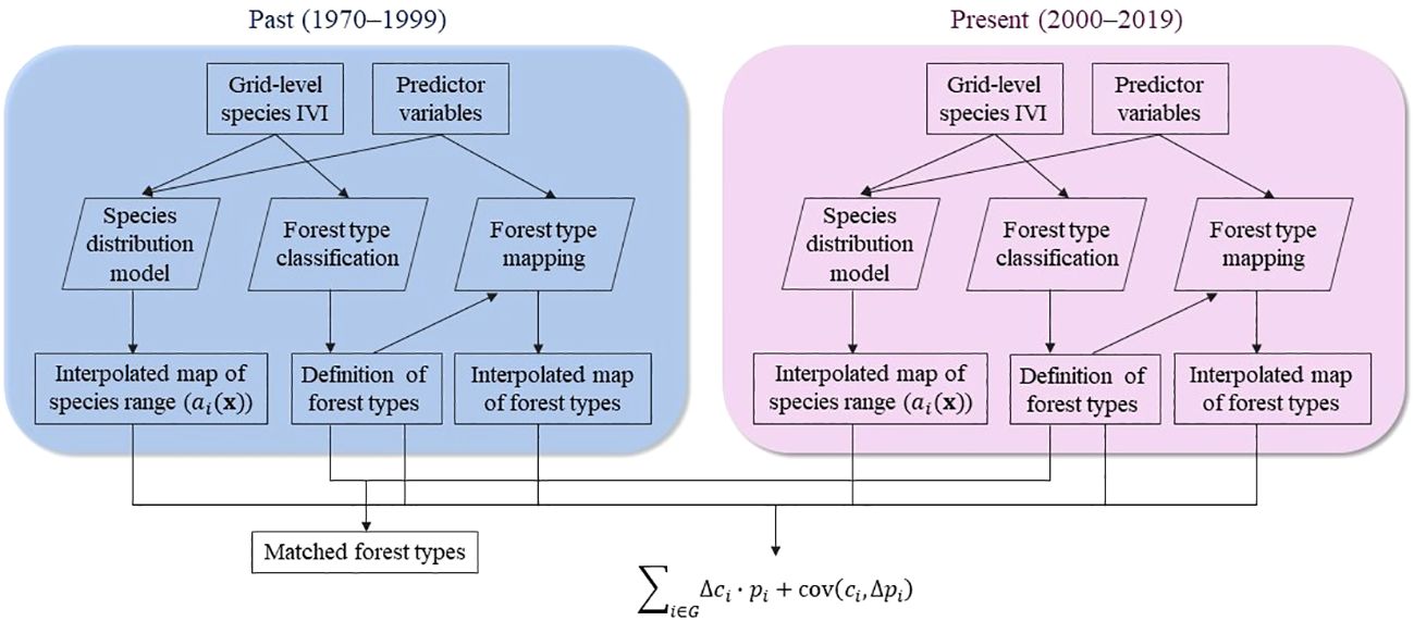
Figure 1 Overview of the methods. Tree data was prepared for each period at the 0.025° grid level (approximately 3km) with species importance value index (IVI). Using the tree data, we built species distribution models to create interpolated maps of species distribution ranges and classified forest types. For each pair of forest types that were identified in both periods, we estimated the range shift of the forest type and the average of constituent species based on the portfolio hypothesis. Species range shift was represented by the geographic centroid shift of the interpolated distributions range.

2.1 The portfolio hypothesis of range shifts

We derived the following hypothesis from Markowitz’s portfolio theory of investment (Markowitz, 1952) to quantify the difference in range shifts between forest types and constituent tree species. Tree species range shift was represented by the geographic centroid shift of its modeled distribution range.

Let $a_i(x)$ be the relative abundance of species $i$ at spatial location $x$ (demarcated by coordinates of latitude and longitude). The cumulative relative abundance of species $i$ over space $x$ is ${\displaystyle {\sum }_x{a}_i(x)}=A_i$, and the geographic centroid of species $i$’s range can be calculated as the weighted mean of $x$, $c_i={\displaystyle {\sum }_{x}x·a_i}(x)/A_i$. The relative abundance of a forest type at location $x$ is the sum of its constituent species’ relative abundance at the location, $a(x)={\displaystyle {\sum }_{i\in G}{a}_i}(x)$, where G = (1,...,n) represents the set of all species of this forest type. The cumulative relative abundance of this forest type can be computed as ${\displaystyle {\sum }_{x}a}(x)=A$; let $p_i=A_i/A$, and the geographic centroid of the forest type can be calculated as $c={\displaystyle {\sum }_{x}x}·a(x)/A={\displaystyle {\sum }_{i\in G}{c}_i}·p_i$. By the Leibniz product rule of calculus (see details in Supplementary Text 1.1), we have

$\begin{array}{ll}\mathrm{\Delta }c={\displaystyle {\sum }_{i\in G}\mathrm{\Delta }{c}_i}·p_i+{\displaystyle {\sum }_{i\in G}{c}_i}·\mathrm{\Delta }{p}_i& (1)\end{array}$

Because ${\displaystyle {\sum }_{i\in G}{p}_i}=1$ and thus ${\displaystyle {\sum }_{i\in G}\mathrm{\Delta }}{p}_i=0$, the latter term of Equation 1 equals the covariance between species’ centroids and the change in their cumulative relative abundance: $\text{cov}(c_i, \mathrm{\Delta }{p}_i)=\text{E}(c_i·\mathrm{\Delta }{p}_i)-\text{E}(c_i)·\text{E}(\mathrm{\Delta }{p}_i)={\displaystyle {\sum }_{i\in G}{c}_i}·\mathrm{\Delta }{p}_i$.

Notably, the shift in a forest type’s centroid ($\mathrm{\Delta }c$) is driven not only by the weighted mean of centroid shifts at the species level (${\displaystyle {\sum }_{i\in G}\mathrm{\Delta }{c}_i·p_i}$), but also, counterintuitively, by the covariance ($\text{cov}(c_i, \mathrm{\Delta }{p}_i)$) that inflates or deflates the centroid shift of the forest type (Figure 2). This covariance term, which we call the portfolio effect, can be attributed to a difference between forest type range shift and the range shift of its constituent tree species. We therefore made the following hypothesis: when the range shift of a forest type and its constituent tree species are measured along a given direction, a positive covariance ($\text{cov}(c_i, \mathrm{\Delta }{p}_i)$) will inflate the magnitude and velocity of the forest type range shift along this direction, while a negative covariance will reduce the magnitude and velocity along this direction (Figure 2). In most cases, portfolio effects are expected to be positive because species at the front of a forest type range (i.e., in the direction of forest type range shift) often have increasing abundances due to preferential allocation to dispersal and reproduction, while species at the rear of forest type range are decreasing in abundance, reflecting the compounded effect of constituent species’ mortality and recruitment on the centroid shift (Burton et al., 2010; Rumpf et al., 2018).

Figure 2

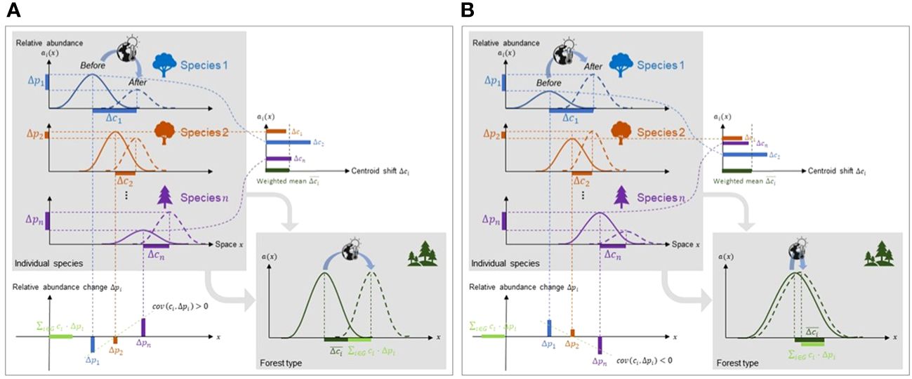
Figure 2 Range shift dynamics of forest type and constituent tree species based on the portfolio effect. Forest type shift is controlled by constituent species centroid shifts ($\text{Δ}{c}_i$) and changes in cumulative relative abundance ($\Delta p_i$). The covariance between a species’ centroid and the change in its cumulative relative abundance ($cov(c_i,\Delta p_i)$) determines whether forest type shift outpaces or lags tree species shifts. (A) In this simple scenario where tree species and forest type shift along the same direction, if covariance > 0, forest type shift outpaces tree species shifts, but (B) if covariance< 0, forest shift is outpaced by tree species shifts.

2.2 Data integration

For this study, we compiled and integrated in situ forest-tree data from independent and standard forest inventories. Data for the United States came from the Forest Inventory and Analysis (FIA) (Burrill et al., 2021) and the Cooperative Alaska Forest Inventory (CAFI) (Malone et al., 2009). Data for Canada came from two independent sources: permanent sample plot networks (Paquette and Messier, 2011; Chen et al., 2016) and Canada’s National Forest Inventory ground plot network (National Forest Inventory, 2011; Zhang et al., 2017). See Supplementary Text 1.2 for a detailed description of each data.

We derived the following data integration protocol to harmonize the different forest inventory datasets described above into consistent continental data frames. From each dataset, we obtained tree-level information for all the trees with a minimum diameter at breast height (DBH) of 1 cm. We grouped these tree-level records by the year of inventory and compiled one data frame for 2000–2019 and another data frame for 1970–1999. For each period, we summarized tree-level information into a plot-level species abundance matrix. We calculated, for each sample plot, the importance value index (IVI hereafter) for a species, which is the sum of the percent number of stems and the percent basal area for the species. Frequently used in forestry research as a typical measure of species abundance (Dyer, 2006; Costanza et al., 2017; Iverson et al., 2019a), IVI equally weighs the number of stems and basal area of a particular species, and ranges from 0 to 200.

The final continental data frames consisted of plot identification and coordinates, as well as the IVIs of all tree species present on each plot. The plots were widely distributed across the forested areas of the continent (Supplementary Figure 1). For the 1970–1999 data frame, because some trees in the genera of Aesculus, Amelanchier, Carya, Crataegus, Halesia, Malus, and Salix were recorded only to the genus level, we also calculated the IVIs of these genera (Supplementary Table 1). To mitigate the impact of sampling bias (Araújo et al., 2019), we derived the average species IVI of all plots located within a 0.025° by 0.025° (approximately 3 by 3 km) grid cell in each past and present plot-level dataset, which is a reasonable aggregation regardless of the distribution of species IVI (see Supplementary Text 1.3).

We also compiled 38 predictor variables for the supervised learning of species and forest type distributions, consisting of 17 climate variables (Fick and Hijmans, 2017; Karger et al., 2017; Trabucco and Zomer, 2019; Karger et al., 2022), 13 topographic variables (Amatulli et al., 2018), seven soil variables (Batjes, 2016), and human footprint (Venter et al., 2016). These predictor variables were derived from open-access satellite-based remote sensing and ground-based survey data layers, all of which have a nominal resolution of 1 km. Detailed information on the predictor variables is available in Supplementary Table 2. Different climate and human footprint data were used for past and present periods to match the represented years (see Supplementary Table 2).

We extracted predictor variables to the centroid of each grid cell using the “sf” or “raster” packages (Pebesma, 2018; Hijmans, 2023; Hijmans and Van Etten, 2022) in R (R Core Team, 2021) and used the “Hmisc” package in R to impute missing data in those predictor variables (Harrell, 2023). Our final training data encompassed more than 114,000 grid cells for the present period and 97,000 grid cells for the past period containing species IVI and 38 predictor variables.

For mapping purposes, we prepared another 0.025° by 0.025° grid, covering forest extent across North America with all predictor variables. Each grid cell had a minimum 10% canopy cover based on the global forest range map (Hansen et al., 2013), in accordance with FAO’s definition of “forest” (FAO, 2020). Species or forest type distributions were predicted for each grid cell of this mapping grid. Our study region encompassed 1,004,358 grid cells of forested area across North America, with a total of ~5 million km². The tropical regions of North America, i.e., Mexico, Central America, and the Caribbean, were not included in this analysis due to a lack of remeasured in situ data.

Our study region covered 92 terrestrial ecoregions (Olson et al., 2001) across the United States and Canada. These ecoregions were grouped into three distinct arch-biomes based on the definition of the eastern United States in previous studies (e.g., Knott et al., 2020) and biome map (Olson et al., 2001): West (39 ecoregions), East (33 ecoregions), and Boreal (20 ecoregions, Supplementary Figure 1). For each arch-biome and time frame (2000–2019 and 1970–1999), we classified forest type (see 2.4 Forest type classification) and quantified distribution ranges of forest types and constituent tree species separately.

2.3 Range shifts of tree species

Following the formulation of the portfolio hypothesis, the first step to quantify forest type range shifts is to determine constituent species’ range shift patterns, which consisted of two steps: creating a spatially continuous map of species $i$‘s relative abundance ($a_i(x)$) at location $x$ (i.e., grid latitude and longitude) across the continent and quantifying its geographic centroid shift ($\mathrm{\Delta }{c}_i$). To estimate a species’ relative abundance, we first created interpolated maps of species IVI across the 4.9 million-km² study region using random forests model and 38 predictor variables, which took similar steps as correlative species distribution models (Araújo et al., 2019; Iverson et al., 2019a). Since we do not have sufficient samples in some areas, we used interpolated relative abundance map instead of observations. For each arch-biome (West, East, and Boreal) and time frame (2000–2019 and 1970–1999), only species with sufficient sample size (≥60 grid cells where species IVI > 0) in both time periods were included (van Proosdij et al., 2016; Supplementary Table 1).

Random forests are a non-parametric ensemble learning approach (Breiman, 2001), which combines a variant of decision trees and an additional level of randomness by bootstrapping sub-data and different sets of predictor variables. Random forests are commonly used in species distribution models (Araújo et al., 2019) as it mitigates the multicollinearity issues that most statistical models face (James et al., 2013). We used the “randomForest” package in R (version 4.0.4) (Liaw and Wiener, 2002) to train a separate model for each species, period, and arch-biome. Following Iverson et al. (2019a), we reported the mean predicted IVI of all decision trees for each species or zero for species with zero median and a coefficient of variation no less than 2.75 among all predicted values of decision trees. For each species, we built 20 random forests models to calculate an average IVI in each grid cell in the mapping grid.

Based on the estimated species IVI, we calculated species relative abundance ($a_i(x)$) along each latitudinal and longitudinal gradient by calculating percent IVI for each species in each grid cell. We then calculated the cumulative relative abundance ($A_i={\displaystyle {\sum }_x{a}_i}(x)$) and geographic centroid ($c_i={\displaystyle {\sum }_{x}x·a_i}(x)/A_i$) for each species. The direction and velocity of species range shift ($\Delta c_i$) were calculated based on the displacement between the past and present geographic centroids using the “sp” and “sfsmisc” packages in R (Pebesma and Bivand, 2005; Maechler et al., 2023). In this study, the direction was measured in azimuth, the angle between past and present geographic centroids around the same horizon (i.e., altitude was not considered), ranging from 0 to 360° measured from the North direction. We also determined the total area of each species’ range as the sum of the grid cell area weighted by the species’ relative abundance. Grid cell area was estimated using the “raster” package in R (Hijmans and Van Etten, 2022).

2.4 Forest type classification

We modified the existing forest type classification algorithm (Dyer, 2006; Costanza et al., 2017) to determine forest type definition in each arch-biome and period. Specifically, instead of hierarchical cluster analysis used in previous research (Dyer, 2006; Costanza et al., 2017), we used K-means cluster analysis due to the size of the data. We first used an autoencoder neural network to calculate a latent space representation of the original grid tree IVI data, which is often more suitable for K-means cluster analysis than the original data (Song et al., 2014). Instead of the interpolated maps of species IVI, we used the grid-level observational data to maximize the performance of cluster analysis. See Supplementary Text 1.4 for a detailed description of autoencoder neural networks and the architecture used in this study. To avoid potential bias caused by insufficient sample sizes, we excluded the species that are present in less than 60 grid cells (where IVI > 0) (Supplementary Table 1).

Based on the reduced dimensional representation, we then conducted a K-means cluster analysis using the built-in function “kmeans” in R (R Core Team, 2021). We set the number of starts to 50 and the maximum iterations to 100. To fine-tune hyperparameters for the autoencoder neural networks (the number of dimensions) and K-means cluster analysis (the number of clusters; Supplementary Figure 2), we calculated the silhouette width using the “cluster” package in R (Maechler, 2018). Silhouette width is an indicator of between-cluster heterogeneity; With a range between −1 and 1, positive silhouette width values indicate that a given member of a cluster is closer to its own cluster’s centroid than to the nearest cluster’s centroid. Negative values indicate that a given member is closer to the nearest cluster’s centroid than to the centroid of its own cluster. Generally, higher silhouette width values indicate greater between-cluster heterogeneity.

With the optimal hyperparameter values, we conducted K-means cluster analysis 20 times to derive the final classification results due to the random nature of the analysis. Since forest types (i.e., clusters) were defined independently in each of the 20 repetitions, we manually matched the same forest type based on similarities in mean species IVI (i.e., species composition for each forest type) between all the combinations of forest types generated from the 20 repetitions. When 10 or more repetitions identified the given forest type, we recognized the forest type as a final forest type. Moreover, since we classified forest types for three arch-biomes separately (West, East, and Boreal), there were potential overlaps of forest types between them. To identify and merge potential overlaps, we calculated the Euclidean distance of all combinations of the final forest types in terms of mean species IVI. If an Euclidean distance was less than 60, forest types across arch-biomes were merged. One exception was that western aspen–mixed conifer (W‐J) and boreal quaking aspen–spruce (B-A) remained separated due to the large expanse of quaking aspen (Populus tremuloides).

Finally, with the final set of forest types for each period, we identified forest types that were present in both periods. To do this, we calculated the Euclidean distance of all combinations between past and present forest types in terms of mean species IVI. Pairs were considered matching when the forest type of minimum distance was the same between the past-and-present pair. For example, if and only if present forest type X’s closest past forest type is Y, and past forest type Y’s closest present forest type is also X, they were considered matching. Finally, we manually grouped final forest types into larger forest biome categories based on Eyre (1980).

2.5 Forest type mapping

We predicted the distribution ranges of forest types by first considering two candidate imputation models: random forests and support-vector machines. Support-vector machines are supervised learning models which construct a hyperplane or set of hyperplanes in a high- or infinite-dimensional space to help analyze data for classification and regression analysis (Vanpik and Cortes, 1995). We used the “e1071” package in R with the default hyperparameter setting (Meyer et al., 2019). For random forests, we used the default hyperparameter setting of the “randomForest” package in R (Liaw and Wiener, 2002) and the same set of predictor variables as described in 2.2. Data integration.

To assess the performance of the imputation model in mapping forest types across the continent, we conducted a rigorous 80/20 cross-validation using bootstrapping. In each iteration, we used stratified sampling to split the entire dataset into the training (80%) and testing (20%) sets and conducted the combination of under-sampling and oversampling of the training set for both random forests and support-vector machines to balance the sample size for all classes (i.e., forest types). Stratified sampling was conducted using the “caret” package in R (Kuhn et al., 2020), and under-sampling and oversampling were conducted using the “UBL” package (Branco et al., 2016). Based on five random iterations with sample replacement in each of the 20 repetitions, we calculated the 95% confidence interval of classification accuracy, the Kappa statistic, and elements of the confusion matrix. For each candidate imputation model, the output was a matrix of class probability from five iterations. We chose the forest type of majority vote from the five iterations, and thus, our final output was a matrix of class probability from the 20 repetitions. Based on how many repetitions, out of 20, returned the given forest type, we calculated percent forest type in each grid cell. Every grid cell has a sum of 100 for all forest types, with the forest type with the highest percentage being the final assigned forest type. (e.g., The final forest type assigned to a grid cell consisting of 20% forest type A, 30% forest type B, and 50% forest type C is forest type C). The percent forest type was used to visualize the geographic patterns of forest type range shifts, species-level range shifts, and the difference between them.

2.6 Range shifts of forest types

Following the formulation of the portfolio hypothesis, we calculated the weighted sum of species-level shifts (${\displaystyle {\sum }_{i\in G}\mathrm{\Delta }{c}_i}·p_i$), the covariance (the portfolio effect, $\text{cov}(c_i, \mathrm{\Delta }{p}_i)$), and the sum of the two (i.e., forest type-level shift ($\mathrm{\Delta }c$)) for each forest type that was present in both periods along the latitudinal and longitudinal gradient. For each forest type, $G$ represents the set of all species present in the forest type (mean species IVI > 0). Along each respective gradient, $\mathrm{\Delta }{c}_i$ represents the centroid shift of species $i$, $\mathrm{\Delta }{p}_i$ represents the change in $p_i$ from past to present periods, and $p_i$ and $c_i$ take the mean values of past and present periods. Thus, we have the species-level shifts, covariance, and forest type-level shift for each latitudinal and longitudinal gradient for each forest type, where the weighted sum of species range shifts (${\displaystyle {\sum }_{i\in G}\mathrm{\Delta }}{c}_i·p_i$) and covariance term ($\text{cov}(c_i, \mathrm{\Delta }{p}_i)$) precisely matches a forest type range shift ($\mathrm{\Delta }c$).

In a two-dimensional space with latitude and longitude combined, we also derived the velocity of a forest type range shift in kilometers per decade and azimuth angle by calculating the distance between past and present forest type centroids using “sp” and “sfsmisc” packages in R (Pebesma and Bivand, 2005; Maechler et al., 2023). This forest type range shift can be visualized as a vector in a two-dimensional space of latitude and longitude, as a resultant of two composing vectors: species-level vector and covariance vector. Quantifying the length of these two vectors (i.e., velocity) is not practical due to the earth’s curvature, yet we aimed to approximate it by calculating the distance between past forest type centroid and the point to where the vector heads, both in degrees and kilometers (see Supplementary Figure 3 for a visualized example). Finally, to expand the velocity of forest type and species range shifts to a grid level for visualization purposes, we weighted the velocity of each forest type by the percent forest type in each grid cell. Average percentage of past and present forest types was used.

3 Results

Our forest type classification identified eight forest biomes and 43 forest types across North America (Figure 3, Supplementary Figures 4–11, Supplementary Table 3). The mean silhouette widths from our K-means cluster analyses were significantly greater than zero for all forest types (p< 0.001) in the West for the present dataset (Supplementary Table 4). Eighteen out of 19 forest types in the West, 22 out of 26 in the East, and all six forest types in the Boreal region were significantly greater than zero in the mean silhouette width. In summary, 90% of the forest types classified here were significantly distinct from one another in terms of species composition (Supplementary Table 4).

Figure 3

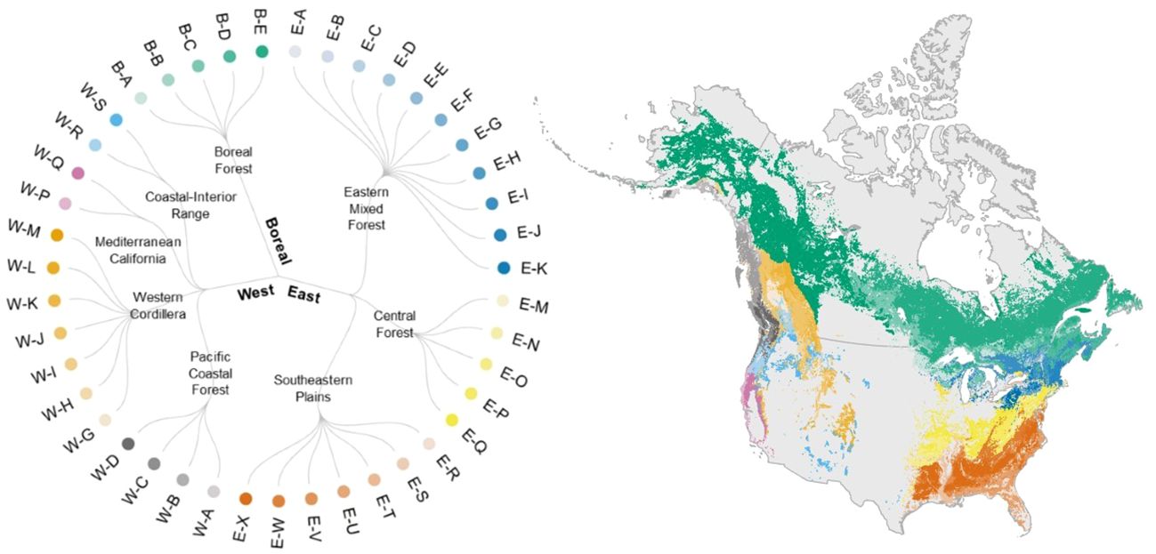
Figure 3 We classified forested areas across North America into 43 forest types in eight forest biomes and three arch-biomes (East, West, and Boreal) following the existing algorithms. See Supplementary Table 3 for the definition of forest types and constituent tree species. Colors in the circular dendrogram corresponds to those in the map of forest type distribution range. Here, we show a map of forest types for the present period, based on the distribution of forest types estimated by random forests (see 2.5 Forest type mapping).

For mapping the ranges of classified forest types, the random forests model was 10–17% and 11–20% more accurate in terms of overall accuracy and the Kappa statistic, respectively, compared with the support vector machine model (Supplementary Figure 12). Therefore, we selected random forests as the final imputation model. The confusion matrices based on random forests models were based on the number of cases in class prediction, standardized in percentage (Supplementary Figures 13, 14). For the present dataset, the coastal redwood–tanoak forest (W-P) had the highest classification accuracy (88%; Supplementary Figure 13), and the red maple–hardwood forest (E-F) had the lowest one (18%; Supplementary Figure 13) among all forest types.

At the individual species level, Sitka spruce (Picea sitchensis) had the greatest velocity in range shifts (480.4 km·decade^-1), followed by balsam fir (Abies balsamea; 438.6 km·decade^-1) and gray alder (Alnus incana; 354.6 km·decade^-1) (Figure 4A, Supplementary Table 1). In contrast, pond cypress (Taxodium ascendens) had the lowest velocity of all (1.5 km·decade^-1), followed by water-elm (Planera aquatica; 4.5 km·decade^-1) and sweetgum (Liquidambar styraciflua; 4.5 km·decade^-1). The velocities of temperate tree species range shifts found in our study are consistent with those reported in the previous studies (Supplementary Table 5). Few boreal tree species have ever been assessed in terms of shifting velocity, and here, we found that boreal tree species’ ranges are shifting much faster than temperate ones. In terms of direction, 36 out of 150 species shifted northwards, 34 eastwards, 27 southwards, and 53 westwards during the studied period (Supplementary Table 1).

Figure 4

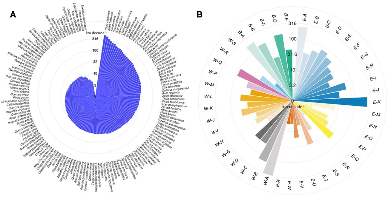
Figure 4 The velocity of (A) tree species range shifts and (B) forest type range shifts. Velocity of shifts (here in logarithmic scale) is defined as the distance between past and present centroids of range in kilometers per decade (km·decade^-1). See Supplementary Table 3 for the definition of forest types and constituent tree species.

At the forest type level, we found that the range of Sitka spruce–western hemlock forest (W-A) shifted with the highest velocity at 327.8 km·decade^-1 (Figure 4B). Among the top six fast-shifting forest types, three were in the boreal forest biome (B-A, B-B, and B-D, see Supplementary Table 3 for forest type names), two were in the eastern mixed forest biome (E-A and E-K), and one was in the Pacific-coastal forest biome (W-B) (Supplementary Table 4). The remaining forest types shifted at a velocity lower than 100 km·decade^-1. In terms of the direction of shift, nine out of 43 forest types shifted westwards, 16 eastwards, 11 southwards, and seven northwards during the studied period (Supplementary Table 4).

Overall, forest type range shifts differed substantially from tree species range shifts (i.e., the average range shift of constituent tree species) in terms of velocity (Figures 5, 6). On average, forest type ranges shifted at 86.5 km·decade^-1, more than three times as fast as the weighted average of their constituent tree species (28.8 km·decade^-1) across the continent at the grid level (Figures 5B, 6C). For more than 75% of forest types, the range shifts at the forest type level substantially outpaced the average range shifts of constituent tree species, and only 10 out of 43 forest types moved more slowly than their constituent tree species in terms of range shifts (Figure 6C, Supplementary Table 4). In the boreal and Great Lakes regions, the velocity of forest type range shifts exceeded that of tree species range shifts by 200 km·decade^-1 or more (Figure 5B). Along the Rocky and Appalachian Mountains, forest type ranges shifted with a lower velocity than the ranges of their constituent tree species (Figure 5B).

Figure 5

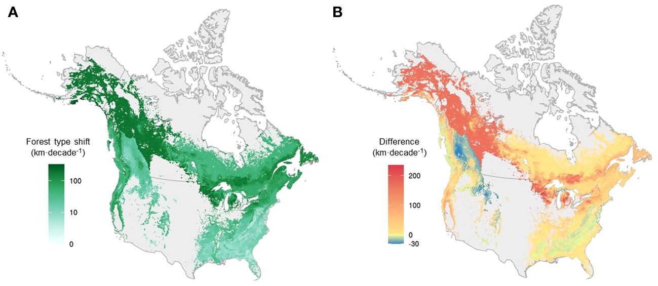
Figure 5 The velocity of forest type range shift and the difference in velocity between forest types and the weighted mean of their constituent species across the continent, mapped at a 0.025° resolution. (A) The velocity of forest type at the grid level. (B) The difference in shift velocity between forest types and the weighted mean of their constituent species at the grid level, with warm colors representing areas where forest type range shifts outpaced species range shifts, and cold colors representing areas where species range shifts outpaced forest type range shifts. Forest type range shift and the weighted mean of its constituent species were first quantified for each forest type. Here, we used interpolated maps of forest types to visualize them based on percent forest type in each grid cell.

Figure 6

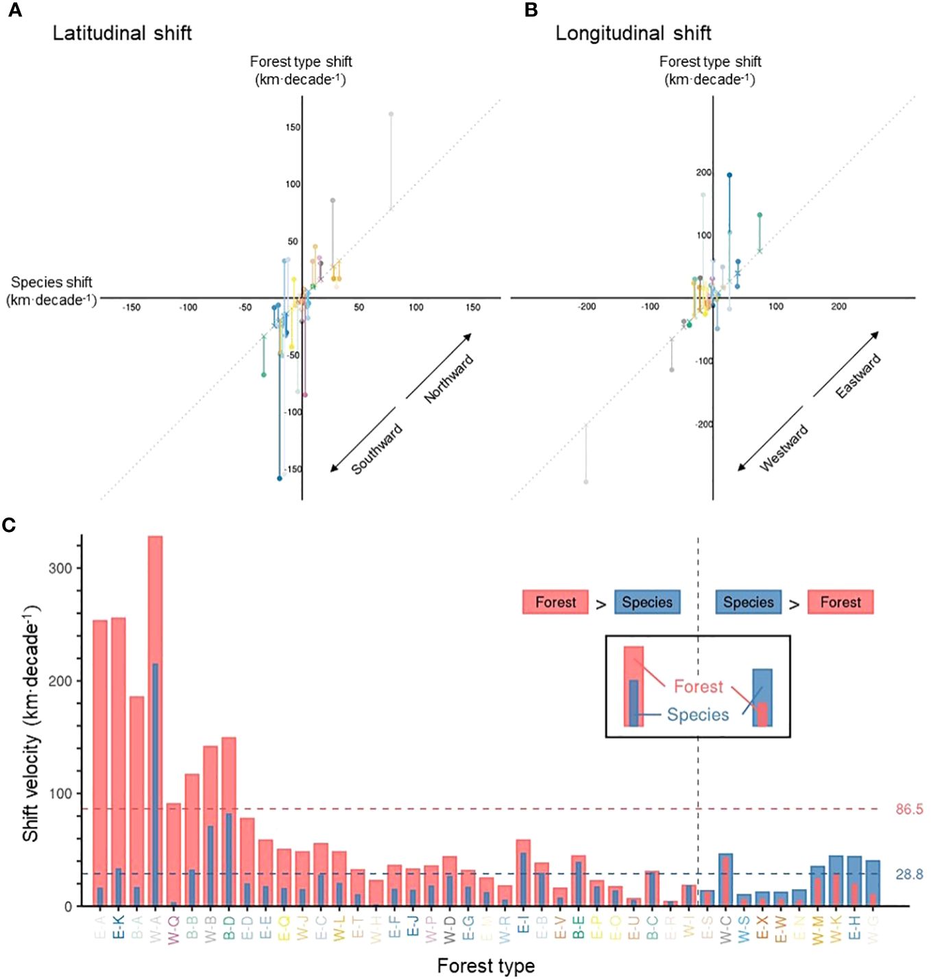
Figure 6 The difference between forest type range shifts and tree species range shifts. Scatter plots show the velocity of forest type vs. tree species range shift velocity, in terms of latitudinal (A) and longitudinal (B) shift of geographic centroids, with positive values representing northward (A) and eastward (B) shifts and negative values southward (A) and westward (B) shifts. Vertical line segments represent the difference between the velocity of forest type range shifts and tree species range shifts, along latitude (A) and longitude (B). The length of these segments is identical to the portfolio effect. (C) A comparison between the velocity of forest type and tree species range shift velocity, regardless of the direction. The horizontal dotted lines represent the mean velocity of forest type and tree species shists in pink and blue, respectively. The mean velocity represents a grid-level velocity (i.e., Figure 5A for forest type). To ease identification of various forest types, axis text colors of the Panel (C) are consistent with Figures 3, 4B.

4 Discussion

While existing forest type classifications for North America are limited to either Canada or the United States (Rowe, 1972; Dyer, 2006; Ruefenacht et al., 2008; Costanza et al., 2017; Knott et al., 2020), our study supports ongoing and future international collaborations in forest management and climate actions (FAO and UNEP, 2020), with a consistent continental-wide data-driven forest type classification scheme. Nevertheless, our classified forest types are generally compatible with existing forest type classifications for the North American continent (Rowe, 1972; Dyer, 2006; Ruefenacht et al., 2008; Costanza et al., 2017; Knott et al., 2020).

Our findings provide strong support for the portfolio hypothesis. The marked difference in the range shift velocity between forest type and constituent tree species is mainly attributable to the covariance term ($\text{cov}(c_i, \mathrm{\Delta }{p}_i)$), which we call the portfolio effect. Positive portfolio effects provide a mechanistic underpinning of our finding that, across the North American continent, forest type range shifts generally outpaced tree species range shifts (Figures 5B, 6C). In some cases, negative covariance terms pervade, leading to reduced forest type range shift, such as in some forests across the Rocky and Appalachian Mountains (Figure 5B). In these montane forest types, constituent species increase their relative abundances in the rear edge, where investments in competitive traits are likely to dominate, even if the species centroids drift towards the front edge (Figure 2).

Various factors in complex interactions are attributable to species abundance dynamics, leading to positive or negative portfolio effects. While climate change (e.g., increasing temperature and precipitation changes) is commonly considered the major driver of species abundance dynamics and associated range shifts (Boisvert-Marsh et al., 2014; Fei et al., 2017; Sittaro et al., 2017), climate change-induced disturbances (e.g., fires and disease outbreaks), human disturbances (e.g., logging and land use changes), and biotic interactions influencing the dispersal and survival rates can further exacerbate the dynamics of species abundance (Vanderwel and Purves, 2014; Anderegg et al., 2015; Gauthier et al., 2015; Brice et al., 2019, 2020; Seidl et al., 2020). Although it is out of the scope of this study to assess the determinants behind species abundance dynamics, we utilized non-climate predictor variables, including human footprint (Venter et al., 2016) (Supplementary Table 2), to account for the impacts of potential human disturbances.

There are profound impacts of forest type range shifts on forest biodiversity and associated ecosystem functioning, food, water, energy security (Gitay et al., 2002; Neilson et al., 2005; Wellstead and Howlett, 2017; Kremen and Merenlender, 2018), human well-being (IPBES, 2018), and socioeconomic value (Hanewinkel et al., 2013). Forest type range shifts can jeopardize the sustainability of local forest industries, making them more vulnerable to timber price fluctuations (Zhou, 2021). It can also inflate timber procurement ranges and increase transportation costs, causing significant downstream financial implications with serious welfare and economic consequences comparable to the impact of COVID-19 on transportation and logistics (Polzin and Choi, 2021). Furthermore, the collective human experiences of rural communities embedded within these forested landscapes have strong ties to surrounding forest types. From the Sitka spruce–western hemlock forests in the Pacific Northwest to the oak–pine forests along the Appalachians (Supplementary Table 4), the change in native forest ecosystems may be threatening the customs, identities, and culture of indigenous (Chamberlain et al., 2018) and other local communities while jeopardizing non-timber forest products supply and overall environmental justice (Fleetwood, 2020). The rapid shift of forest types may place urgency on human communities, especially rural populations, to adapt their cultural norms and relationships with surrounding forests.

Our finding that a majority of forest types shifted faster than their constituent tree species due to positive portfolio effects suggests that the impacts of tree species’ range shifts under global change on forest ecosystem functioning and services may be underestimated. Forest ecosystem functioning (Loreau, 2000; Cardinale et al., 2011), productivity (Liang et al., 2016), phenology, and population turnover (Zhu et al., 2014; Pecl et al., 2017) are directly related to tree species composition and other forest characteristics (Loreau, 2000; Cardinale et al., 2011; Paquette and Messier, 2011; Liang et al., 2016). Therefore, existing adaptive forest management regimes, which are based primarily on individual species range projections and associated environmental and social aspects (Millar et al., 2007; Iverson et al., 2019b), may have underestimated the impacts of global change (including climate change, land use change, invasive species regimes, habitat fragmentation, and forest degradation). Compositional changes of species into novel forest types imply that forest managers may need to address effects on forest ecosystems that are unique in space and time (Iverson and McKenzie, 2013), pursuant to a need for more dynamic silvicultural practices. For instance, in the central United States, a diminishing supply of various white oak species, such as white oak (Quercus alba) and bur oak (Q. macrocarpa), is threatening the bourbon industry (Conrad et al., 2019), a staple of American culture and tradition. These oak species are supported by a variety of co-existing tree species; For example, deep roots of hickory species (Carya spp.) improve soil structure (Smith, 2024), eastern redbud (Cercis canadensis) enhance soil nutrient availability through nitrogen fixation, pine species (Pinus spp.) co-exist without intense competition (Nowacki and Abrams, 2008), and species like black cherry (Prunus serotina) support a wide range of wildlife species, which play a critical role in acorn dispersal. Shifts and contracting ranges of these co-existing species communities can negatively affect the quality and volume of oak species for local industry. As forest type-level change (25% reduction in Appalachian oak–pine forest range, Supplementary Table 4) was far more apparent than species-level change (e.g., 12.5% reduction in Q. alba range and 6% increase in Q. macrocarpa range, Supplementary Table 1), missing the forest for the trees for their range shift patterns may reduce the capability and preparedness of local forest industry and communities to face global change through disruptions in timber supply chains and ecosystem benefits.

Positive portfolio effects enable us to scale global change-induced range shifts up to the levels where decision-making processes often take place. Because of the portfolio effect, climate change and other factors of global change, such as anthropogenic effects, land use change, as well as associated insects/disease outbreaks and invasive species regimes, will result not only in the migration of forest types, but also in the emergence of new forest types (Williams and Jackson, 2007). Due to unequal changes in relative abundance among species, new assemblages of species (i.e., new forest types that are unknown today) may appear. To this end, additional research could outline the relative importance of various global change factors on forest migration and tree species range shift patterns. Further spatial analyses could also disentangle directional and non-directional factors influencing the absolute difference in range shift velocity between forest types and constituent tree species.

In this study, we quantified the velocity of range shifts using interpolated maps over a large geographic area to best assess the difference between forest type range shifts and constituent species range shifts. As such, some species in our results exhibited higher velocities than previously reported. This is especially prominent in the boreal region, where sample density is limited (Supplementary Figure 1) and no previous studies have ever assessed at this spatial scale. The contrast between our reported velocities and previous studies mainly results from three sources: uncertainty associated with interpolation, limitations in incorporating biotic factors into species distribution, and the spatial scale of this study. While estimating the distributions of species or similar entities through interpolation or extrapolation has been a popular method in ecology (Araújo et al., 2019), predictions are subject to various uncertainties (Beale and Lennon, 2012), which could affect the reported velocities. Nevertheless, we minimized the uncertainty associated with sampling bias through grid aggregation, model selection by considering several candidate models, and extrapolation by analyzing three arch-biomes separately. However, the incorporation of biotic interactions (competition, dispersal ability, etc.) remains an enormous challenge in correlative distribution modeling (Araújo et al., 2019), and thus, the interpolated maps do not reflect realized niche but rather suitable areas for species or forest types in terms of climate, topography, and soil characteristics. Our study also covers a larger geographic area than previous studies, and we were able to capture the entire range of species or forest types without being limited by political boundaries. Nevertheless, our main objective was the comparison between forest type range shifts and constituent species range shifts, and the use of interpolated maps enabled an effective comparison at a large geographic scale.

The divergent range shift patterns between forest types and tree species observed here represent only a snapshot of a more prominent trend seen in geological time scales. Forests, because of their sensitivity to changes in tree species compositions, have over the millennia exhibited shorter life spans than individual species (Williams et al., 2004). Positive portfolio effects may provide a critical scientific basis for adaptive forest management and conservation in mitigating the impacts of rapid forest transformation under climate change.

Data availability statement

Publicly available datasets were analyzed in this study. Grid-level input data with tree species IVI for each region (West, East, and Boreal) for each time frame (2000–2019 and 1970–1999) to reproduce the results, as well as the output forest type and biome maps (geoTIFF layers), are available through Figshare (https://doi.org/10.6084/m9.figshare.22825313.v1). The forest inventory data used in this study includes publicly available data: Forest Inventory and Analysis (FIA) (https://apps.fs.usda.gov/fia/datamart/datamart.html), permanent sample plots for Québec (https://www.donneesquebec.ca/recherche/dataset/placettes-echantillons-permanentes-1970-a-aujourd-hui), and Canada’s National Forest Inventory (https://nfi.nfis.org/en). The predictor variables used in this study are all openly available; climate covariates are available through WorldClim (https://www.worldclim.org/data/worldclim21.html), CHELSA (https://chelsa-climate.org/bioclim/), and Trabucco and Zomer (2019) (https://figshare.com/articles/dataset/Global_Aridity_Index_and_Potential_Evapotranspiration_ET0_Climate_Database_v2/7504448/4), topographic covariates are available through EarthEnv (https://www.earthenv.org/topography), soil covariates are available through WISE30sec (https://data.isric.org/geonetwork/srv/eng/catalog.search#/metadata/dc7b283a-8f19-45e1-aaed-e9bd515119bc), and human footprint layer is available from Venter et al. (2016) (https://doi.org/10.5061/dryad.052q5).

Author contributions

AA: Conceptualization, Data curation, Formal analysis, Investigation, Methodology, Software, Validation, Visualization, Writing – original draft, Writing – review & editing. CW: Investigation, Writing – original draft, Writing – review & editing. JG: Investigation, Writing – original draft, Writing – review & editing. CH: Conceptualization, Writing – original draft, Writing – review & editing. NP: Conceptualization, Writing – original draft, Writing – review & editing. TO: Investigation, Writing – original draft, Writing – review & editing. SM: Writing – original draft, Writing – review & editing. RS: Methodology, Writing – original draft, Writing – review & editing. SF: Writing – original draft, Writing – review & editing. AP: Data curation, Writing – original draft, Writing – review & editing. HC: Data curation, Writing – original draft, Writing – review & editing. AC: Writing – original draft, Writing – review & editing. JL: Conceptualization, Data curation, Funding acquisition, Investigation, Methodology, Project administration, Resources, Supervision, Visualization, Writing – original draft, Writing – review & editing.

Funding

The author(s) declare financial support was received for the research, authorship, and/or publication of this article. This work was supported by the U.S. Department of Agriculture’s (USDA) Agricultural Marketing Service [grant numbers AM200100XXXXG007]; USDA National Institute of Food and Agriculture McIntire Stennis project 1017711; Start-up Fund provided by the Department of Forestry and Natural Resource and the College of Agriculture, Purdue University; Department of Forestry and Natural Resources, Purdue University; Takenaka Scholarship Foundation; Natural Sciences and Engineering Research Council of Canada [grant numbers RGPIN-2019–05109, STPGP506284]; and Serra-Húnter Fellowship provided by the Government of Catalonia.

Acknowledgments

We thank the Global Forest Biodiversity Initiative (GFBI) and Science-i.org for facilitating the international research collaboration. We thank Mo Zhou and John B. Dunning, Jr. for their feedback on this study.

Conflict of interest

The authors declare that the research was conducted in the absence of any commercial or financial relationships that could be construed as a potential conflict of interest.

Publisher’s note

All claims expressed in this article are solely those of the authors and do not necessarily represent those of their affiliated organizations, or those of the publisher, the editors and the reviewers. Any product that may be evaluated in this article, or claim that may be made by its manufacturer, is not guaranteed or endorsed by the publisher.

Supplementary material

The Supplementary Material for this article can be found online at: https://www.frontiersin.org/articles/10.3389/fevo.2024.1366568/full#supplementary-material

References

Amatulli G., Domisch S., Tuanmu M. N., Parmentier B., Ranipeta A., Malczyk J., et al. (2018). A suite of global, cross-scale topographic variables for environmental and biodiversity modeling. Sci. Data 5, 180040. doi: 10.1038/sdata.2018.40

PubMed Abstract | CrossRef Full Text | Google Scholar

Anderegg W. R., Hicke J. A., Fisher R. A., Allen C. D., Aukema J., Bentz B., et al. (2015). Tree mortality from drought, insects, and their interactions in a changing climate. New Phytol. 208, 674–683. doi: 10.1111/nph.13477

PubMed Abstract | CrossRef Full Text | Google Scholar

Araújo M. B., Anderson R. P., Barbosa A. M., Beale C. M., Dormann C. F., Early R., et al. (2019). Standards for distribution models in biodiversity assessments. Sci. Adv. 5, eaat4858. doi: 10.1126/sciadv.aat4858

PubMed Abstract | CrossRef Full Text | Google Scholar

Batjes N. H. (2016). Harmonized soil property values for broad-scale modelling (WISE30sec) with estimates of global soil carbon stocks. Geoderma 269, 61–68. doi: 10.1016/j.geoderma.2016.01.034

CrossRef Full Text | Google Scholar

Beale C. M., Lennon J. J. (2012). Incorporating uncertainty in predictive species distribution modelling. Philos. Trans. R. Soc Lond. B Biol. Sci. 367, 247–258. doi: 10.1098/rstb.2011.0178

PubMed Abstract | CrossRef Full Text | Google Scholar

Boisvert-Marsh L., Périé C., De Blois S. (2014). Shifting with climate? Evidence for recent changes in tree species distribution at high latitudes. Ecosphere 5, 1–33. doi: 10.1890/ES14-00111.1

CrossRef Full Text | Google Scholar

Branco P., Ribeiro R. P., Torgo L. (2016) UBL: an R package for utility-based learning. Available online at: http://arxiv.org/abs/1604.08079.

Google Scholar

Breiman L. (2001). Random forests. Mach. Learn. 45, 5–32. doi: 10.1023/A:1010933404324

CrossRef Full Text | Google Scholar

Brice M. H., Cazelles K., Legendre P., Fortin M. J. (2019). Disturbances amplify tree community responses to climate change in the temperate–boreal ecotone. Glob. Ecol. Biogeogr. 28, 1668–1681. doi: 10.1111/geb.12971

CrossRef Full Text | Google Scholar

Brice M. H., Vissault S., Vieira W., Gravel D., Legendre P., Fortin M. J. (2020). Moderate disturbances accelerate forest transition dynamics under climate change in the temperate–boreal ecotone of eastern North America. Glob. Change Biol. 26, 4418–4435. doi: 10.1111/gcb.15143

CrossRef Full Text | Google Scholar

Burrill E. A., Ditommaso A. M., Turner J. A., Pugh S. A., Christensen G., Perry C. J., et al. (2021). The forest inventory and analysis databse: database description and user guide version 9.0.1 for phase 2 (Washington, DC, USA: U.S. Department of Agriculture, Forest Service). Available at: https://www.fia.fs.usda.gov/library/database-documentation/current/ver91/FIADB%20User%20Guide%20P2_9-1_final.pdf.

Google Scholar

Burton O. J., Phillips B. L., Travis J. M. (2010). Trade-offs and the evolution of life-histories during range expansion. Ecol. Lett. 13, 1210–1220. doi: 10.1111/j.1461-0248.2010.01505.x

PubMed Abstract | CrossRef Full Text | Google Scholar

Cardinale B. J., Matulich K. L., Hooper D. U., Byrnes J. E., Duffy E., Gamfeldt L., et al. (2011). The functional role of producer diversity in ecosystems. Am. J. Bot. 98, 572–592. doi: 10.3732/ajb.1000364

PubMed Abstract | CrossRef Full Text | Google Scholar

Cavender-Bares J., Kozak K. H., Fine P. V. A., Kembel S. W. (2009). The merging of community ecology and phylogenetic biology. Ecol. Lett. 12, 693–715. doi: 10.1111/j.1461-0248.2009.01314.x

PubMed Abstract | CrossRef Full Text | Google Scholar

Chamberlain J. L., Emery M. R., Patel-Weynand T. (2018). Assessment of nontimber forest products in the United States under changing conditions (Ashville, NC, USA: U.S. Department of Agriculture, Forest Service, Southern Research Station). doi: 10.2737/SRS-GTR-232

CrossRef Full Text | Google Scholar

Chen H. Y., Luo Y., Reich P. B., Searle E. B., Biswas S. R. (2016). Climate change-associated trends in net biomass change are age dependent in western boreal forests of Canada. Ecol. Lett. 19, 1150–1158. doi: 10.1111/ele.12653

PubMed Abstract | CrossRef Full Text | Google Scholar

Chen I. C., Hill J. K., Ohlemüller R., Roy D. B., Thomas C. D. (2011). Rapid range shifts of species associated with high levels of climate warming. Science 333, 1024–1026. doi: 10.1126/science.1206432

PubMed Abstract | CrossRef Full Text | Google Scholar

Chesson P., Donahue M. J., Melbourne B. A., Sears A. L. (2005). ““Scale transition theory for understanding mechanisms in metacommunities,”,” in Metacommunities: spatial dynamics and ecological communities. Eds. Holyoak M., Leibold M. A., Holt R. D. (University of Chicago Press, Chicago, IL), 279–306.

Google Scholar

Clements F. E. (1916). Plant succession: an analysis of the development of vegetation (Washington, D.C: Carnegie Institution of Washington).

Google Scholar

Conrad A. O., Crocker E. V., Li X., Thomas W. R., Ochuodho T. O., Holmes T. P., et al. (2019). Threats to oaks in the eastern United States: perceptions and expectations of experts. J. For. 118, 14–27. doi: 10.1093/jofore/fvz056

CrossRef Full Text | Google Scholar

Costanza J. K., Coulston J. W., Wear D. N. (2017). An empirical, hierarchical typology of tree species assemblages for assessing forest dynamics under global change scenarios. PloS One 12, e0184062. doi: 10.1371/journal.pone.0184062

PubMed Abstract | CrossRef Full Text | Google Scholar

Dyer J. M. (2006). Revisiting the deciduous forests of eastern North America. BioScience 56, 341–352. doi: 10.1641/0006-3568(2006)56[341:RTDFOE]2.0.CO;2

CrossRef Full Text | Google Scholar

Eyre F. H. (1980). Forest cover types of the United States and Canada (Wachington D.C: Society of American Foresters).

Google Scholar

FAO. (2020). Global forest resources assessment 2020 (Rome, Italy). Available at: https://www.fao.org/3/ca9825en/ca9825en.pdf.

Google Scholar

FAO, UNEP. (2020). The state of the world’s forests 2020 (Rome, Italy: Forests, biodiversity and people). Available at: https://www.unep.org/resources/state-worlds-forests-forests-biodiversity-and-people.

Google Scholar

Fei S., Desprez J. M., Potter K. M., Jo I., Knott J. A., Oswalt C. M. (2017). Divergence of species responses to climate change. Sci. Adv. 3, e1603055. doi: 10.1126/sciadv.1603055

PubMed Abstract | CrossRef Full Text | Google Scholar

Fick S. E., Hijmans R. J. (2017). WorldClim 2: new 1-km spatial resolution climate surfaces for global land areas. Int. J. Climatol. 37, 4302–4315. doi: 10.1002/joc.5086

CrossRef Full Text | Google Scholar

Fleetwood J. (2020). Social justice, food loss, and the Sustainable Development Goals in the era of COVID-19. Sustainability 12, 5027. doi: 10.3390/su12125027

CrossRef Full Text | Google Scholar

Gauthier S., Bernier P., Kuuluvainen T., Shvidenko A. Z., Schepaschenko D. G. (2015). Boreal forest health and global change. Science 349, 819–822. doi: 10.1126/science.aaa9092

PubMed Abstract | CrossRef Full Text | Google Scholar

Gitay H., Suarez A., Watson R. (2002). Climate change and biodiversity (Geneva, Switzerland: International Panel on Climate Change). Available at: https://www.ipcc.ch/site/assets/uploads/2018/03/climate-changes-biodiversity-en.pdf.

Google Scholar

Gleason H. A. (1926). The individualistic concept of the plant association. Bull. Torrey Bot. Club 53, 7–26. doi: 10.2307/2479933

CrossRef Full Text | Google Scholar

Guisan A., Zimmermann N. E. (2000). Predictive habitat distribution models in ecology. Ecol. Modell. 135, 147–186. doi: 10.1016/S0304-3800(00)00354-9

CrossRef Full Text | Google Scholar

Hanewinkel M., Cullmann D. A., Schelhaas M.-J., Nabuurs G.-J., Zimmermann N. E. (2013). Climate change may cause severe loss in the economic value of European forest land. Nat. Clim. Change 3, 203–207. doi: 10.1038/nclimate1687

CrossRef Full Text | Google Scholar

Hansen M. C., Potapov P. V., Moore R., Hancher M., Turubanova S. A., Tyukavina A., et al. (2013). High-resolution global maps of 21st-century forest cover change. Science 342, 850–853. doi: 10.1126/science.1244693

PubMed Abstract | CrossRef Full Text | Google Scholar

Harrell F. Jr. (2023). “Hmisc: Harrell miscellaneous,” in R package version 5.1-0. Available at: https://CRAN.R-project.org/package=Hmisc.

Google Scholar

Hijmans R. (2023). “raster: Geographic data analysis and modeling,” in R package version 3.6-26. Available at: https://CRAN.R-project.org/package=raster.

Google Scholar

Hijmans R., Van Etten J. (2022). “raster: Geographic data analysis and modeling,” in R package version 3.6-11. Available at: https://cran.r-project.org/web/packages/raster/index.html.

Google Scholar

Hui C., Fox G. A., Gurevitch J. (2017). Scale-dependent portfolio effects explain growth inflation and volatility reduction in landscape demography. Proc. Natl. Acad. Sci. U.S.A. 114, 12507–12511. doi: 10.1073/pnas.1704213114

PubMed Abstract | CrossRef Full Text | Google Scholar

IPBES. (2018). Report of the plenary of the Intergovernmental Science-Policy Platform on Biodiversity and Ecosystem Services on the work of its sixth session (Medellín, Colombia: IPBES). Available at: https://files.ipbes.net/ipbes-web-prod-public-files/downloads/ipbes-6-15-add.4-advance_eca.pdf.

Google Scholar

Iverson L. R., McKenzie D. (2013). Tree-species range shifts in a changing climate: detecting, modeling, assisting. Landsc. Ecol. 28, 879–889. doi: 10.1007/s10980-013-9885-x

CrossRef Full Text | Google Scholar

Iverson L. R., Peters M. P., Prasad A. M., Matthews S. N. (2019a). Analysis of climate change impacts on tree species of the eastern US: Results of DISTRIB-II modeling. Forests 10, 302. doi: 10.3390/f10040302

CrossRef Full Text | Google Scholar

Iverson L. R., Prasad A. M., Peters M. P., Matthews S. N. (2019b). Facilitating adaptive forest management under climate change: A spatially specific synthesis of 125 species for habitat changes and assisted migration over the eastern United States. Forests 10, 989. doi: 10.3390/f10110989

CrossRef Full Text | Google Scholar

James G., Witten D., Hastie T., Tibshirani R. (2013). An introduction to statistical learning (New York: Springer). doi: 10.1007/978-1-4614-7138-7

CrossRef Full Text | Google Scholar

Karger D. N., Conrad O., Böhner J., Kawohl T., Kreft H., Soria-Auza R. W., et al. (2017). Climatologies at high resolution for the earth’s land surface areas. Sci. Data 4, 1–20. doi: 10.1038/sdata.2017.122

CrossRef Full Text | Google Scholar

Karger D. N., Conrad O., Böhner J., Kawohl T., Kreft H., Soria-Auza R. W., et al. (2022). Data from: Climatologies at high resolution for the earth’s land surface areas (Dryad Digital Repository). doi: 10.5061/dryad.kd1d4

CrossRef Full Text | Google Scholar

Kelly A. E., Goulden M. L. (2008). Rapid shifts in plant distribution with recent climate change. Proc. Natl. Acad. Sci. U.S.A. 105, 11823–11826. doi: 10.1073/pnas.0802891105

PubMed Abstract | CrossRef Full Text | Google Scholar

Knott J. A., Jenkins M. A., Oswalt C. M., Fei S. (2020). Community-level responses to climate change in forests of the eastern United States. Glob. Ecol. Biogeogr 29, 1299–1314. doi: 10.1111/geb.13102

CrossRef Full Text | Google Scholar

Kremen C., Merenlender A. M. (2018). Landscapes that work for biodiversity and people. Science 362, eaau6020. doi: 10.1126/science.aau6020

PubMed Abstract | CrossRef Full Text | Google Scholar

Küchler A. W. (1964). Potential natural vegetation of the conterminous United States (New York: American Geographical Society).

Google Scholar

Kuhn M. (2008). Building predictive models in R using the caret package. J. Stat. Softw. 28 (5), 1–26. doi: 10.18637/jss.v028.i05

CrossRef Full Text | Google Scholar

Lenoir J., Gegout J. C., Marquet P. A., De Ruffray P., Brisse H. (2008). A significant upward shift in plant species optimum elevation during the 20th century. Science 320, 1768–1771. doi: 10.1126/science.1156831

PubMed Abstract | CrossRef Full Text | Google Scholar

Liang J., Crowther T. W., Picard N., Wiser S., Zhou M., Alberti G., et al. (2016). Positive biodiversity-productivity relationship predominant in global forests. Science 354, aaf8957. doi: 10.1126/science.aaf8957

PubMed Abstract | CrossRef Full Text | Google Scholar

Liang J., Gamarra J. G. P. (2020). The importance of sharing global forest data in a world of crises. Sci. Data 7, 424. doi: 10.1038/s41597-020-00766-x

PubMed Abstract | CrossRef Full Text | Google Scholar

Liaw A., Wiener M. (2002). Classification and regression by randomForest. R News 2, 18–22.

Google Scholar

Loreau M. (2000). Biodiversity and ecosystem functioning: recent theoretical advances. Oikos 91, 3–17. doi: 10.1034/j.1600-0706.2000.910101.x

CrossRef Full Text | Google Scholar

Maechler M., Rousseeuw P., Struyf A., Hubert M., Hornik K. (2023). Cluster Analysis Basics and Extensions. R package version 2.1.6. Available at https://CRAN.R-project.org/package=cluster

Google Scholar

Maechler M., et al. (2024). Utilities from 'Seminar fuer Statistik. ETH Zurich. Zurich, Switzerland. R package version 1.1-17. Available at: https://CRAN.R-project.org/package=sfsmisc

Google Scholar

Malone T., Liang J., Packee E. C. (2009). Cooperative Alaska forest inventory (U.S. Department of Agriculture, Forest Service, Pacific Northwest Research Station). doi: 10.2737/PNW-GTR-785

CrossRef Full Text | Google Scholar

Markowitz H. M. (1952). Portfolio selection. J. Finance 7, 77–91.

Google Scholar

Meyer D., Dimitriadou E., Hornik K., Weingessel A., Leisch F., Chang C.-C., et al. (2019). “e1071: misc functions of the department of statistics, probability theory group (formerly: E1071), TU Wien,” in R package version, 1. Available at: https://CRAN.R-project.org/package=e1071.

Google Scholar

Millar C. I., Stephenson N. L., Stephens S. L. (2007). Climate change and forests of the future: managing in the face of uncertainty. Ecol. Appl. 17, 2145–2151. doi: 10.1890/06-1715.1

PubMed Abstract | CrossRef Full Text | Google Scholar

National Forest Inventory. (2011). Canada’s National Forest Inventory – ground plot data (Canada’s National Forest Inventory). Available at: https://nfi.nfis.org/en.

Google Scholar

Neilson R. P., Pitelka L. F., Solomon A. M., Nathan R., Midgley G. F., Fragoso J. M. V., et al. (2005). Forecasting regional to global plant migration in response to climate change. BioScience 55, 749–759. doi: 10.1641/0006-3568(2005)055[0749:FRTGPM]2.0.CO;2

CrossRef Full Text | Google Scholar

Nowacki G. J., Abrams M. D. (2008). ). The demise of fire and “Mesophication” of forests in the eastern United States. BioScience 58, 123–138. doi: 10.1641/B580207

CrossRef Full Text | Google Scholar

Olson D. M., Dinerstein E., Wikramanayake E. D., Burgess N. D., Powell G. V. N., Underwood E. C., et al. (2001). Terrestrial ecoregions of the world: A new map of life on Earth: A new global map of terrestrial ecoregions provides an innovative tool for conserving biodiversity. BioScience 51, 933–938. doi: 10.1641/0006-3568(2001)051[0933:TEOTWA]2.0.CO;2

CrossRef Full Text | Google Scholar

Paquette A., Messier C. (2011). The effect of biodiversity on tree productivity: from temperate to boreal forests. Glob. Ecol. Biogeogr. 20, 170–180. doi: 10.1111/j.1466-8238.2010.00592.x

CrossRef Full Text | Google Scholar

Pebesma E. (2018). Simple features for R: Standardized support for spatial vector data. R J. 10, 439–446. doi: 10.32614/RJ-2018-009

CrossRef Full Text | Google Scholar

Pebesma E., Bivand R. S. (2005). Classes and methods for spatial data: the sp package. R News 5, 9–13.

Google Scholar

Pecl G. T., Araujo M. B., Bell J. D., Blanchard J., Bonebrake T. C., Chen I. C., et al. (2017). Biodiversity redistribution under climate change: Impacts on ecosystems and human well-being. Science 355, aai9214. doi: 10.1126/science.aai9214

CrossRef Full Text | Google Scholar

Perry C. H., Finco M. V., Wilson B. T. (2022). Forest atlas of the United States (U.S. Department of Agriculture, Forest Service, Northern Research Station). Available at: https://www.fs.usda.gov/sites/default/files/fs_media/fs_document/Forest-Atlas-of-the-United-States.pdf.

Google Scholar

Polzin S., Choi T. (2021). COVID-19’s effects on the future of transportation (U.S. Department of Transportation, Office of the Assistant Secretary for Research and Technology). doi: 10.21949/1520705

CrossRef Full Text | Google Scholar

R Core Team. (2021). R: A language and environment for statistical computing (Vienna, Austria: R Foundation for Statistical Computing).

Google Scholar

Rowe J. S. (1972). Forest regions of Canada (Ottawa, ON, Canada: Fisheries and Environment Canada, Canadian Forest Service).

Google Scholar

Ruefenacht B., Finco M. V., Nelson M. D., Czaplewski R., Helmer E. H., Blackard J. A., et al. (2008). Conterminous U.S. and Alaska forest type mapping using Forest Inventory and Analysis data. Photogramm. Eng. Remote Sens. 11, 1379–1388. doi: 10.14358/PERS.74.11.1379

CrossRef Full Text | Google Scholar

Rumpf S. B., Hulber K., Klonner G., Moser D., Schutz M., Wessely J., et al. (2018). Range dynamics of mountain plants decrease with elevation. Proc. Natl. Acad. Sci. U.S.A. 115, 1848–1853. doi: 10.1073/pnas.1713936115

PubMed Abstract | CrossRef Full Text | Google Scholar

Schindler D. E., Armstrong J. B., Reed T. E. (2015). The portfolio concept in ecology and evolution. Front. Ecol. Environ. 13, 257–263. doi: 10.1890/140275

CrossRef Full Text | Google Scholar

Seidl R., Honkaniemi J., Aakala T., Aleinikov A., Angelstam P., Bouchard M., et al. (2020). Globally consistent climate sensitivity of natural disturbances across boreal and temperate forest ecosystems. Ecography 43, 967–978. doi: 10.1111/ecog.04995

CrossRef Full Text | Google Scholar

Sharma S., Andrus R., Bergeron Y., Bogdziewicz M., Bragg D. C., Brockway D., et al. (2022). North American tree migration paced by climate in the West, lagging in the East. Proc. Natl. Acad. Sci. U.S.A. 119, e2116691118. doi: 10.1073/pnas.2116691118

PubMed Abstract | CrossRef Full Text | Google Scholar

Sittaro F., Paquette A., Messier C., Nock C. A. (2017). Tree range expansion in eastern North America fails to keep pace with climate warming at northern range limits. Glob. Change Biol. 23, 3292–3301. doi: 10.1111/gcb.13622

CrossRef Full Text | Google Scholar

Smith H. C. (2024) Carya cordiformis (Wangenh.) (Bitternut Hickory). Available online at: https://www.srs.fs.usda.gov/pubs/misc/ag_654/volume_2/carya/cordiformis.htm (Accessed February 14, 2024).

Google Scholar

Song C., Huang Y., Liu F., Wang Z., Wang L. (2014). Deep auto-encoder based clustering. Intell. Data Anal. 18, S65–S76. doi: 10.3233/IDA-140709

CrossRef Full Text | Google Scholar

Steidinger B. S., Crowther T. W., Liang J., Van Nuland M. E., Werner G. D. A., Reich P. B., et al. (2019). Climatic controls of decomposition drive the global biogeography of forest-tree symbioses. Nature 569, 404–408. doi: 10.1038/s41586-019-1128-0

PubMed Abstract | CrossRef Full Text | Google Scholar

Trabucco A., Zomer R. (2019). Data from: Global Aridity Index and Potential Evapotranspiration (ET0) Climate Database v2. figshare. doi: 10.6084/m9.figshare.7504448.v2

CrossRef Full Text | Google Scholar

Vanderwel M. C., Purves D. W. (2014). How do disturbances and environmental heterogeneity affect the pace of forest distribution shifts under climate change? Ecography 37, 10–20. doi: 10.1111/j.1600-0587.2013.00345.x

CrossRef Full Text | Google Scholar

Vanpik V., Cortes C. (1995). Support-vector networks. Mach. Learn. 20, 273–297. doi: 10.1007/BF00994018

CrossRef Full Text | Google Scholar

van Proosdij A. S. J., Sosef M. S. M., Wieringa J. J., Raes N. (2016). Minimum required number of specimen records to develop accurate species distribution models. Ecography 39, 542–552. doi: 10.1111/ecog.01509

CrossRef Full Text | Google Scholar

Venter O., Sanderson E. W., Magrach A., Allan J. R., Beher J., Jones K. R., et al. (2016). Sixteen years of change in the global terrestrial human footprint and implications for biodiversity conservation. Nat. Commun. 7, 12558. doi: 10.1038/ncomms12558

PubMed Abstract | CrossRef Full Text | Google Scholar

Wellstead A., Howlett M. (2017). Assisted tree migration in North America: policy legacies, enhanced forest policy integration and climate change adaptation. Scand. J. For. Res. 32, 535–543. doi: 10.1080/02827581.2016.1249022

CrossRef Full Text | Google Scholar

Williams J. W., Jackson S. T. (2007). Novel climates, no-analog communities, and ecological surprises. Front. Ecol. Environ. 5, 475–482. doi: 10.1890/070037

CrossRef Full Text | Google Scholar

Williams J. W., Shuman B. N., Webb Iii T., Bartlein P. J., Leduc P. L. (2004). Late-quaternary vegetation dynamics in North America: Scaling from taxa to biomes. Ecol. Monogr. 74, 309–334. doi: 10.1890/02-4045

CrossRef Full Text | Google Scholar

Woodall C. W., Oswalt C. M., Westfall J. A., Perry C. H., Nelson M. D., Finley A. O. (2009). An indicator of tree migration in forests of the eastern United States. For. Ecol. Manage. 257, 1434–1444. doi: 10.1016/j.foreco.2008.12.013

CrossRef Full Text | Google Scholar

Woodall C. W., Oswalt C. M., Westfall J. A., Perry C. H., Nelson M. D., Finley A. O. (2010). Selecting tree species for testing climate change migration hypotheses using forest inventory data. For. Ecol. Manage. 259, 778–785. doi: 10.1016/j.foreco.2009.07.022

CrossRef Full Text | Google Scholar

Zhang Y., Chen H. Y. H., Taylor A. R. (2017). Positive species diversity and above-ground biomass relationships are ubiquitous across forest strata despite interference from overstorey trees. Funct. Ecol. 31, 419–426. doi: 10.1111/1365-2435.12699

CrossRef Full Text | Google Scholar

Zhou M. (2021). Input substitution and relative input price variability in timber markets. Can. J. For. Res. 51, 339–347. doi: 10.1139/cjfr-2020-0338

CrossRef Full Text | Google Scholar

Zhu K., Woodall C. W., Clark J. S. (2012). Failure to migrate: lack of tree range expansion in response to climate change. Glob. Change Biol. 18, 1042–1052. doi: 10.1111/j.1365-2486.2011.02571.x

CrossRef Full Text | Google Scholar

Zhu K., Woodall C. W., Ghosh S., Gelfand A. E., Clark J. S. (2014). Dual impacts of climate change: forest migration and turnover through life history. Glob. Change Biol. 20, 251–264. doi: 10.1111/gcb.12382

CrossRef Full Text | Google Scholar