MelSPPNET—A self-explainable recognition model for emerald ash borer vibrational signals

1 Introduction

The protection of forestry resources hinges on the prevention and control of plant diseases and insect pests. Among these pests, stem borers are particularly challenging to manage due to their covert lifestyle, prolonged damage period, and delayed symptoms. The emerald ash borer (EAB) is a prominent stem borer pest, as its larvae feed on the inner bark of trees, causing hidden damage (MacFarlane and Meyer, 2005; Kovacs et al., 2010; Mwangola et al., 2022). By the time visible signs of infestation appear, it is often too late to effectively control the outbreak. This makes prevention and control measures extremely difficult (Poland and McCullough, 2006; Ward et al., 2021; Davydenko et al., 2022). In China, the prevalence of single-species tree plantations creates a simplistic forest structure, rendering large-scale plantations vulnerable to EAB infestations.

Traditional methods of pest detection, such as manual searches for adult insects within designated sample plots and performing counts, as well as employing pheromone trapping techniques that involve the use of color-attractant traps, girdled-tree semiochemical attractant traps, and pheromone traps (Rutledge, 2020), remote sensing (Zhou et al., 2022), and image detection, provide valuable information for pest control. However, these methods may not be effective for early detection of pests such as the EAB, whose larvae's feeding stage causes significant damage to the host without noticeable symptoms (Murfitt et al., 2016). The lagging response characteristics of EAB damage and the difficulty of early detection with naked eyes can cause irreparable losses (McCullough and Katovich, 2004). Therefore, the development of sound recognition technology has opened up new possibilities for pest identification. For example, scholars have used the AED-2000 to record the activity sounds of the Red Palm Weevil and the AED-2010 equipment with SP-1L probe to monitor the Grape Root Moth (Inyang et al., 2019; Wang B. et al., 2021; Shi et al., 2022). Nowadays, a convenient and fast detection method involves using the AED instrument to collect vibrations from trees, inputting these into a deep learning model, and then using a neural network model to identify if a tree has been infested by insects. This method can detect pests in the larval stage and save a lot of manual judgment (Wang B. et al., 2021). In addition, the development of neural networks has led to the emergence of pest monitoring and identification based on speech recognition technology. Compared to early methods of recording feeding sounds in the air using fixed sensors on tree trunks, piezoelectric vibration sounds generated by pest activity are more sensitive and less noisy. The vibration signal of the wood borer can be recorded by a sensor and saved in audio format, and feature points can be identified and classified using deep learning technology (Kahl et al., 2018; Liu et al., 2022).

The current development of neural networks is very rapid and has applications in many fields, but in many key areas that require high performance, there are also high requirements for the transparency and interpretability of the model. In various fields such as healthcare (DeGrave et al., 2021; Gautam et al., 2022b), driverless driving (Omeiza et al., 2021), and law (Rudin, 2019), high reliability of algorithms is crucial. However, the lack of transparency and interpretability of models often hinders their practical application, especially when it comes to understanding the reasons for wrong decisions. For these reasons, this also leads to the emergence of explainable artificial intelligence (XAI), which is divided into two lines in the field of explainable artificial intelligence. On the one hand, it is the posteriori interpretation of existing black-box models, that is, the ex post facto explainable method ; on the other hand, some specialized models are being developed to provide predictions and explanations, also known as self-explainable models (SEMs) (Gautam et al., 2022a). And the model we proposed is a self-explanatory model.

In existing XAI research, a study has focused on understanding how traditional convolutional networks recognize vibrational signals by utilizing layer-wise relevance propagation(LRP). They aim to provide pixel-level representations of which values in the input signal contribute the most to the diagnostic outcomes, thus offering post-hoc explanations of how CNNs differentiate between fault types (Grezmak et al., 2019). Another line of research involves designing new network layers using various algorithms, which are applied to convolutional networks for image recognition. These layers are designed to extract different categories of case examples. Based on the similarity between input data and these case examples, they aim to achieve case-based interpretability (Chen et al., 2019; Kim et al., 2021; Liu et al., 2021; Wang J. et al., 2021; Donnelly et al., 2022; Cai et al., 2023). Furthermore, a study employs Variational Autoencoder (VAE) techniques in the field of image recognition. It trains VAEs to generate the average case example images and incorporates these generated cases into the decision-making process. This approach assesses the similarity between input images and cases to achieve interpretability (Gautam et al., 2022a). Additionally, a study introduces a novel interpretation algorithm that assesses the significance of different audio segments in making accurate predictions. This approach offers a scalable and unbiased method to enhance model interpretability in vibration signal recognition (Shah et al., 2022). In summary, there is currently a lack of self-explanatory models for vibration signal recognition, based on the existing research. Therefore, building upon prior studies, we propose MelSPPNET, a case-based Explainable Artificial Intelligence model for the recognition of EAB based on vibrational signals.

2 Related work

The recognition of vibration signals generated by pests can be divided into two stages. In the first stage, human auditory recognition and judgment of the vibration signals generated by pests during feeding are performed in the time-frequency domain. However, this process requires the professional skills of inspectors and may result in misjudgment when environmental noise is very loud. The second stage involves collecting sound or vibration signals and identifying pests through the Internet of Things (Jiang et al., 2022) or algorithms (Du, 2019). Machine learning is an important automatic identification method that uses large amounts of data to find patterns from the original data, classify and predict new input data through these patterns. For instance, Sutin et al. (2019) designed an algorithm for the automatic detection of pulses from Anoplophora glabripennis and Agrilus planipennis larvae, whose parameters were typical signals evoked by larvae. When the detected pulse signal exceeds a certain threshold, it can be concluded that the tree is infected. Neural network algorithms are the most widely used in machine learning, and recent advancements in neural network technology have shown that artificial intelligence can solve various complex tasks and even complete some professional tasks (Luo et al., 2022).

Zhu and Zhang (2012) used existing sound parameterization techniques for speech recognition to identify pests. In their research, Mel-scale Frequency Cepstral Coefficients (MFCCs) were extracted from the preprocessed audio data and then classified using a trained Gaussian mixture model (GMM). Sun et al. (2020) proposed a lightweight convolutional neural network containing only four convolutional layers and used keyword discovery technology to recognize the vibrations of Semanotus bifasciatus and Eucryptorrhynchus brandti larvae. All of the models and methods mentioned above are black-box models that can be used for pest identification.

Existing research on the interpretability of neural networks focuses on post-hoc interpretability methods that have evolved from machine learning, such as CAM (Class Activation Maps) (Zhou et al., 2016), LRP (Grezmak et al., 2019), SHAP (SHapley Additive exPlanations) (Lundberg and Lee, 2017), and LIME (Interpretable Model-agnostic Explanations) (Ribeiro et al., 2016). These techniques are applied to pre-trained models to explain how the model classifies input samples into output classes. The post-hoc interpretable methods mentioned above can, to some extent, provide explanations for pre-trained models by interpreting the results and the reasons leading to those results. However, they are not designed for recognition based on patterns similar to human recognition.

Existing SEM models are mostly applied to image recognition, and case-based models such as ProtoPNet (Chen et al., 2019), TesNet (Wang J. et al., 2021), and XProtoNet (Kim et al., 2021) demonstrate excellent performance in bird and medical X-ray prototype recognition. These methods extract prototypes as image patches, using these patches as cases for recognition. However, applying these models to audio recognition does not preserve the original spatial positional information of the prototypes. For audio, the prototypes obtained from these models do not retain the true physical meaning, especially when dealing with spectrograms—images sensitive to spatial positions (i.e., frequency ranges). The patches they obtain lack genuine physical significance for spectrograms. ProtoPNet generates prototypes using training data, and experiments show instances where the same prototype is generated for identical training data (Gautam et al., 2022a). On the other hand, ProtoVAE, based on VAE (Gautam et al., 2022a), generates class-averaged images, addressing the issue of duplicate class prototypes seen in ProtoPNet. This enhances the model's recognition accuracy and robustness in image recognition SEM models. However, when applied to the audio recognition domain with spectrograms as model input, it is constrained by the features of VAE. While it can generate spectrograms with the same frequency range and duration as the original input training data, due to variations in the timing and amplitude of vibration signals in the training samples, the images produced by VAE are merely blurry, averaged representations of the training samples. They cannot serve as interpretable class representatives for humans and lack genuine physical significance.

Currently, there is a lack of SEMs that are suitable for analyzing pest vibration signals. Although traditional black box models can achieve recognition results, they cannot guarantee the reliability and credibility of the model. SEMs that are tailored for pest vibration signals can not only reliably identify trees containing pests but also play a significant role in pest control. However, researchers have not yet applied SEMs to vibration identification of pests. In our study, we focused on the feeding cavity vibration signal of EAB and designed a case-based SEM to achieve reliable identification of the EAB vibration signal.

3 Materials and methods

3.1 Dataset and processing

3.1.1 EAB vibration signal collection

As the vibration signal used to identify EAB is primarily the weak vibration caused by EAB larvae gnawing on the phloem of trees, it is necessary to embed the probe into the tree during the acquisition of EAB larval signal. Voltage transducers are used to collect vibration signals, which are then stored as single-channel audio. Embedding the collection probe into the tree trunk not only reduces the complexity of data collection, but also reduces the interference of environmental noise to a certain extent and improves the purity of the EAB larval vibration. To mitigate training complexity and enhance the representativeness of the prototypes, this study utilized four distinct datasets. The first dataset comprised EAB larval vibrational signals collected in the field, amidst environmental noise. The second dataset consisted solely of environmental noise collected at the same field locations. The third dataset involved vibrational signals from tree sections containing EAB larvae, gathered in a soundproof indoor environment. The fourth dataset encompassed tree noise from soundproof indoor environments, where EAB larvae were absent. The environmental noise collected at field locations and the tree noise in soundproof indoor environments were collectively categorized as environmental noise, with a 2:1 ratio between the two signal types. The first two signal types were collected from the same tree, at varying heights and different positions on trees of the same height in the field, ensuring diversity within the vibration signal categories.

The data collection for the experiments was conducted in a forest area affected by EAB larvae in Tongzhou District, Beijing, from July 18, 2021. The average temperature during the 5-day period was around 33 degrees Celsius. In the North China region, EAB becomes active in mid to late April during the period of sap flow. Pupation begins in late April, and adults emerge in mid-May, with peak emergence occurring from late May to early June. After emergence, adults remain in the pupal chamber for 5–15 days before breaking through the “D”-shaped emergence hole. Newly emerged adults rely on feeding on leaves for about a week to supplement nutrients, causing irregular notches in the foliage. From mid-June to mid-July, adults mate and lay eggs, with an egg incubation period of 7–9 days. Initially, we examined trees exhibiting significant growth disparities compared to others and searched for “D”-shaped emergence holes to identify high-probability ash trees parasitized by EAB larvae. Subsequently, we employed piezoelectric vibration sensors to probe the tree trunk sections. Prior to recording, manual monitoring was conducted to detect larval activity by using headphones.

Recordings were made for approximately one and a half hours daily if larvae activity was observed within each tree trunk. After outdoor collection, the trees were felled and transported to a soundproofed indoor environment where the temperature was ~28 degrees Celsius. Six segments of trees containing EAB larval vibrational signals were collected. Each section was ~30 centimeters in length, and the probe was inserted at the midpoint of the tree trunk. The computer, probe, and tree trunk were positioned on a regular table. Prior to recording, headphones were used to monitor larval activity to confirm their activity. Once the recording commenced, all personnel vacated the room. For live trees where larvae activity was present, vibrational data was recorded daily for an hour and a half. Multiple audio segments were recorded at various times from distinct sections of the tree trunks. As a control measure, the dataset also contained two segments without EAB larvae. These portions primarily contained background noise from the instrument, as there was no larval activity. Recordings began on July 23, 2021, and lasted for five days.

Following data collection, supervised by forestry experts, the bark of all tree sections was removed, revealing the EAB larvae inside and quantifying their count. In two tree segments, there were ~5 to 10 larvae, while the other four segments contained about 10–20 larvae. The larvae were ~3 cm in length, as depicted in Figures 1, 2.

Figure 1

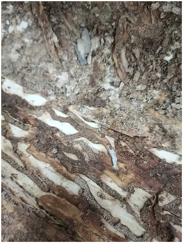
Figure 1. EAB larvae feeding on the phloem.

Figure 2

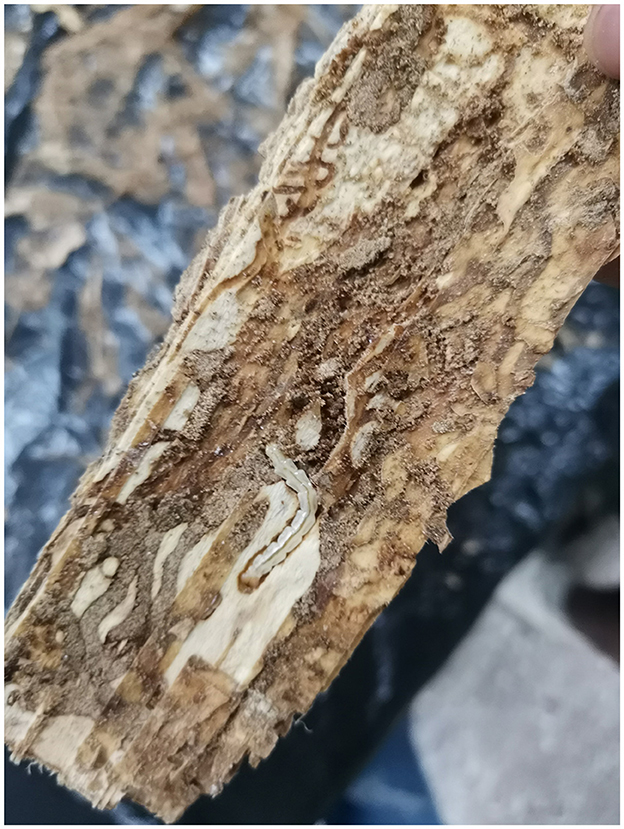
Figure 2. EAB larvae feeding on the phloem visible after removing the bark.

For EAB larval vibration signals containing environmental noise from the collection site, we manually screened and selected audio segments with clear EAB larval vibration signals. All collected data was cut into 5-s audio segments, and a portion of the training data was randomly selected and set as the training and validation sets for model training using a 5:1 ratio. The data was presented in Table 1. The label “0” represents vibration signals containing EAB larvae, while “1” represents vibration signals without EAB larvae.

Table 1

Table 1. Dataset composition.

We use a voltage sensor probe with a sampling frequency of 44.1 kHz and a sampling accuracy of 16bit for signal acquisition. The probe is inserted into the tree trunk to capture the vibration signal directly.

3.1.2 Preprocessing of EAB vibration signal

Similar to many commonly used methods, we utilized Mel spectrogram to simulate the perception of sound by the human ear and extract features from the audio segment. As the EAB larval vibration signal is a non-periodic signal that changes over time, it is necessary to perform a fast Fourier transform, i.e., short-time Fourier transform (STFT), to obtain the spectrogram on several window segments of the new signal. It has been found that humans do not perceive frequency on a linear scale; rather, they are better at detecting differences in lower frequencies rather than higher frequencies. The Mel scale, which is derived from mathematical operations on frequency, better matches the human ear's perception of frequency differences. Therefore, we chose Mel spectrogram as one of the objectives of this study is to learn how the human ear captures EAB larval vibration signals.

Firstly, the sampling rate was set to 16 kHz, and the vibration signal was randomly cropped into audio segments of ≤ 3 s in length for training purposes. If the audio segment was <3 s, it was padded with zeros to 3 s, and the vibration signal was pre-enhanced. Then, the input signal was processed into frames with a frame length of 512 and a step size of 160. The frames were then separated using the Hanning window to ensure that the frequency spectrum was not lost. The short-time Fourier transform was performed on each frame signal, and the absolute value squared was obtained. Finally, the signal was filtered through 80 groups of Mel filters and subjected to discrete cosine transform to obtain the final features. As shown in Figure 3, the feature size was 80 × 301, with the transformed time frames of 301 serving as the length of the feature, and 80 groups of Mel filters serving as the number of channels. This allowed for the transformation of the features from two-dimensional to one-dimensional, making full use of the temporal and spectral information contained within the Mel filter groups. To facilitate human understanding, the feature map was output as a spectrogram, but this did not affect the original features' temporal and spectral information.

Figure 3

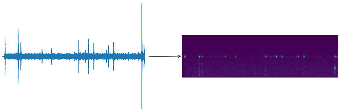
Figure 3. Transformation of vibration signals with random cropping to 301 × 80 Mel feature maps.

3.2 MelSPPNET architecture

Our work is closely related to the case-based classification technique using prototypes, similar to the “visual bag of words” model in image recognition. Our MelSPPNET learns a set of prototypes and compares them with unseen audio segments during the recognition process. Our network uses a specialized neural network architecture for feature extraction and prototype learning, trained in an end-to-end manner. Due to the characteristics of EAB vibration signals, the collected EAB vibration signals are irregular and have uncertain energy. The feature positions of each audio segment are different, and our prototype extraction does not extract the entire training sample of audio that best represents the class, but selects slices of audio samples for finer-grained comparison.

Our network structure consists of two components, one is the traditional convolutional layer, and the other is the prototype layer that extracts prototypes from the training samples, which is used for recognizing vibration signals in a traditional way.

The architectue of the MelSPPNET is shown in the Figure 4. The first part of our network is a conventional convolutional neural network f, whose parameters are collectively denoted as w_conv, followed by a prototype layer g_p and a fully connected layer h with weight matrix w_h but no bias. For the conventional convolutional network f, VGG-16, VGG-19, ResNet-18 or ResNet-34 models can be used as convolutional layers, and two additional 1 × 1 convolutional layers are added in our experiments. Except for the last layer using sigmoid as the activation function, ReLU (rectified linear unit) is used as the activation function for all other convolutional layers.

Figure 4

Figure 4. MelSPPNET architecture.

For a given input vibration signal x, the convolutional layer of our model extracts useful features f(x) for classification. Let H × W denote the shape of the Mel spectrogram of x after preprocessing, where H (mainly containing frequency domain information) is regarded as the number of channels, and the converted time frames W are regarded as the length. Thus, let C × L denote the shape of the output f(x), where the number of output channels C satisfies C ≥ W. After training to a certain extent, the network learns m prototypes $P={\left\{P_j\right\}}_{j=1}^m$, with shape C × L1, where L1 ≤ L. In our experiment, we use L1 = 1. Since the number of channels of each prototype is the same as the number of output channels, but the length of each prototype is less than the length of the entire convolutional output, the prototypes essentially represent subsegments of the convolutional output. These prototypes can be seen as small segments of time in terms of Mel values. Therefore, each prototype will be used to represent some prototype audio patchs in the convolutional output block. Therefore, in this case study, each prototype p_j can be understood as a potential audio patch of the vibration signal.

The process of network training and recognition is illustrated in the Figure 5. Given a convolutional output z = f(x), the j-th prototype unit g_pj in the prototype layer g_p computes the squared L² distance between all audio sub-segments with the same length as p_j in z and p_j, and inverts the distance to a similarity score. The result is an activation matrix of similarity scores, where the value of each element represents the strength of the corresponding prototype part in the audio. The activation matrix preserves the position information of the convolutional output, and can be upsampled to the size of the input matrix to represent the key time frames used for classification and their importance. Using global max pooling reduces the activation matrix generated by each prototype unit g_pj to a single similarity score, which can be understood as the presence of the prototype part in a certain patch of the input audio. The prototype unit g_pj computes the prototype z that is closest to the potential patch p_j by continuously optimizing the parameters. If the output of the j-th prototype unit g_pj is large, there is a patch in the convolutional output that is very similar to the j-th prototype in the latent space, indicating that there is an audio segment in the input audio that is similar to the concept represented by the j-th prototype.

Figure 5

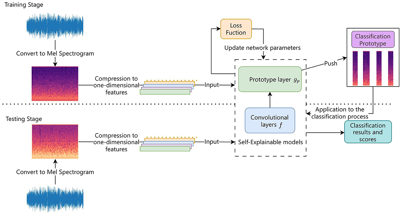
Figure 5. Flowchart of training and testing process.

In our network, we assigned m prototypes for each of the two categories: vibration signals with and without EAB presence (in our experiment, each category has five prototypes). These prototypes are intended to capture the most relevant parts for recognizing these two types of vibration signals.

Finally, the prototype layer g_p generates m similarity scores, which are multiplied by the weight matrix w_h in the fully connected layer h to produce output logits. These logits are then normalized using softmax to generate prediction probabilities for different classes of the given audio. The formula is expressed as follows:softmax(w_hg_p(z)).

3.3 Training model

During the training of our MelSPPNET, we first apply stochastic gradient descent (SGD) to the convolutional layers before the final layer, followed by prototype projection, and finally convex optimization for the last layer.

The SGD optimization in the convolutional layers before the final layer aims to learn a meaningful latent space in which the most important signal patches for vibration signal classification are clustered around prototypes with L² distance in the semantic vicinity of the vibration signal's true class, and clusters with prototypes centered on different classes are well separated. To achieve this effect, we jointly optimize the convolutional layer parameters w_conv and the prototypes in the prototype layer g_p with SGD, while keeping the weights w_h in the last layer fixed. In this process, our objective is to solve the optimization problem, as shown in Equation (1):

$\begin{array}{cc}{\displaystyle \underset{P,w_{conv}}{min}}\frac{1}{n}{\displaystyle \sum _{i=1}^n}CrsEnt(h\circ g_p\circ f(x_i),y_i)+{\lambda }_{1}Clst+{\lambda }_{2}Sep& (1)\end{array}$

Clst and Sep are defined as shown in Equation (2) and Equation (3)

$\begin{array}{cc}Clst=\frac{1}{n}{\displaystyle \sum _{i=1}^n}{\displaystyle \underset{j:p_j\in P_{y_i}}{min}}{\displaystyle \underset{z\in patchs(f(x_i))}{min}}\parallel z-p_j{\parallel }_2^2& (2)\end{array}$

$\begin{array}{cc}Sep=-\frac{1}{n}{\displaystyle \sum _{i=1}^n}{\displaystyle \underset{j:p_j\notin P_{y_i}}{min}}{\displaystyle \underset{z\in patchs(f(x_i))}{min}}\parallel z-p_j{\parallel }_2^2& (3)\end{array}$

Like other networks, the cross-entropy loss (CrsEnt) is used to penalize misclassification of the training data. Minimizing the clustering cost (Clst) encourages each training vibration signal to have some potential patches that are close to at least one prototype of its own class, while minimizing the classification cost (Sep) encourages each potential patch of the training vibration signal not to belong to prototypes of its own class. These losses form a semantically meaningful clustering structure in the latent space, making it easier for the network to classify based on the L² distance.

During this training stage, we also fixed the last layer h whose weight matrix is denoted as w_h. Let $w_h^{(k,j)}$ represent the weight linking the output of the j-th prototype unit g_pj to the logit of class k. For a given class k, we initialized these weights at the first iteration as follows Equation (4):

$\begin{array}{ll}\{\begin{array}{ll}{w}_h^{(k,j)}=1,& p_j\in P_k\\ w_h^{(k,j)}=-0.5,& p_j\notin P_k\end{array}& (4)\end{array}$

where P_k denotes the set of prototypes belonging to class k.

Intuitively, the positive connection between the k-class prototype and the k-class logit means that the similarity with the k-class prototype should increase the predicted probability of the image belonging to the k-class, while the negative connection between the non-k-class prototype and the k-class logit means that the similarity with non-k-class prototype should decrease the predicted probability of the image being classified as the k-class. Fixing the last layer h forces the network to learn a meaningful latent space, as if a latent audio segment of a k-class vibration signal is too close to a non-k-class prototype, it reduces the predicted probability of the segment belonging to the k-class, thus increasing the cross-entropy loss in the training objective. Both the separation cost between the non-k-class prototypes and the k-class logit and the negative connections encourage k-class prototypes to represent semantic concepts that have k-class features rather than other features: if k-class prototypes also represent semantic concepts in non-k-class vibration signals, then the non-k-class vibration signals will highly activate the k-class prototype and be penalized by increasing the separation cost and cross-entropy loss.

3.3.1 Prototype projection

In order to visualize the prototypes as patches of training audio segments, we project (“push”) each prototype p_j onto the nearest latent training patch that belongs to the same class as p_j. This allows us to conceptually equate each prototype with a slice of a training audio segment. Mathematically, for a prototype p_j belonging to class k, i.e., p_j ∈ P_k, we perform the following update, as shown in Equation (5):

$\begin{array}{cc}{p}_j\leftarrow arg{\displaystyle \underset{z\in Z_j}{min}}\parallel z-p_j{\parallel }_2& (5)\end{array}$

where Z_j is defined as Equation (6)

$\begin{array}{cc}{Z}_j=\left\{\tilde{z}:\tilde{z}\in patchs(f(x_i))\forall is.t.y_i=k\right\}& (6)\end{array}$

If the prototype projection does not move the prototypes too far (which is ensured by optimizing the clustering cost Clst), the predictions for the samples that the model correctly predicted with a certain confidence before projection will not change.

Due to the reuse of training samples multiple times as a dataset in training loops, the same patch may be extracted for different batches in different loops, which requires orthogonalization of prototype vectors to achieve intra-class diversity. Without further regularization, prototypes may collapse to the center of the class, excluding the possibility of additional prototypes. To prevent this and promote intra-class diversity, we enforce orthogonality among prototypes within each class, as shown in Equation (7):

$\begin{array}{cc}{L}_{orth}={\displaystyle \sum _{k=1}^K}\parallel {\bar{\Phi }}_k^T{\bar{\Phi }}_k-I_M{\parallel }_F^2& (7)\end{array}$

where I_M is the M × M identity matrix, and the column vectors of matrix ${\bar{\Phi }}_k$ are obtained by subtracting the mean of the prototypes assigned to class k from each prototype, i.e., $\bar{\Phi }k=\varphi kj-\bar{\varphi }k,j=1..M$, where $\bar{\varphi }k=\sum {i=1}^M\varphi ki$. In addition to the traditional regularization using the Frobenius norm ∥·∥_F on the prototypes, this approach promotes separation of the concepts captured within each class, which is one way to achieve intra-class diversity.

Figure 6A shows the prototype obtained by training without adding orthogonal loss, in which two prototypes can be seen to be duplicated, and Figure 6B shows the prototype obtained by training with orthogonal loss added, without duplicated prototypes.

Figure 6

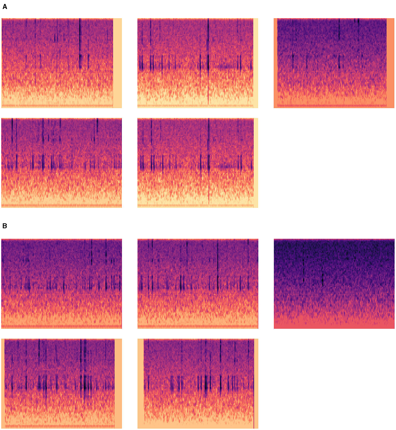
Figure 6. Comparison of prototypes obtained with or without adding orthogonal loss training. (A) Prototype of EAB-containing vibration signal obtained without orthogonal loss training. (B) Prototype of EAB-containing vibration signal obtained with orthogonal loss training.

3.4 Audioization of prototypes

Given a prototype p_j and a training vibration signal x, in the process of prototype projection, we use its latent patch as p_j and use the patch of x's vibration signal highly activated by p_j as the audio representation of p_j. The reason is that the patch of x corresponding to p_j should be the patch with the strongest activation by p_j. We can transform x using a trained MelSPPNET and upsample the activation matrix generated by the prototype unit g_pj before maxpooling to the size of the vibration signal x, in order to find the patch of x that is most highly activated by p_j. The most highly activated patch of x is represented by the high-activation region in the upsampled activation matrix. Then, we audio-ize p_j using the smallest matrix patch of x that surrounds the time interval corresponding to the activation values in the upsampled activation matrix corresponding to g_pj that are at least as high as the 95th percentile of all activation values in that matrix.

3.5 Reasoning process of our network

The Figure 7 shows the inference process of our MelSPPNET when classifying vibration signals containing EAB. Given a test vibration signal x, our model compares its latent feature f(x) with the learned prototypes. Specifically, for each class k, our network attempts to find evidence that x belongs to class k by comparing its latent patch representation with each learned prototype p_j of that class. For example, in the Figure 7, our network tries to find evidence of a vibration signal containing EAB by comparing the latent patch of the vibration signal with each prototype of that class. This comparison produces a matrix of similarity scores for each prototype, which is upsampled and overlaid on the original audio to see which parts of the given vibration signal are activated by each prototype. As shown in the activation matrix column in the Figure 7, the vibration signal to be recognized corresponds to each audio segment of its respective class and is marked on the original audio segment - this is the vibration signal patch that the network considers to sound like the corresponding prototype. In this case, our network found high similarity with different prototypes in the given vibration signal at different time periods. These similarity scores are weighted and added together to give the final score for belonging to that class. The inference process for classes of vibration signals without EAB is also similar.

Figure 7

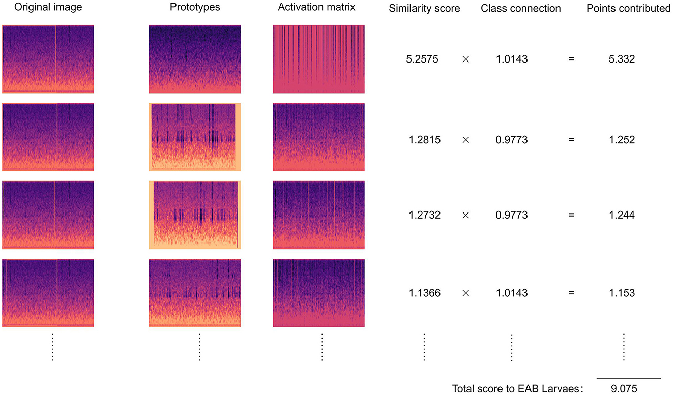
Figure 7. Reasoning process.

3.6 Interpretation score

In order to better evaluate the interpretability of our model, we conducted an evaluation process shown in Figure 8. We used an Interpretation-Score (IS) to measure the interpretability performance of the model. After feeding test data into the trained interpretable recognition model, the model outputs a significance score s for each time frame. By setting a significance threshold ŝ, we count the time frames with significance scores higher than the threshold as key frames, and calculate the sum of significance scores of all key frames as the model's significance score. In addition to significance, we erase the key frames filtered by the threshold from the test data, and feed the remaining data into the model for classification. We then calculate the difference ΔCS between the classification score before and after erasing the key frames. The correlation coefficient between the significance score and the difference in classification scores is used as the model's IS. The significance score reflects the degree of significance of the erased region, while the difference in classification scores reflects the contribution of the erased region to the model's recognition. Therefore, the correlation coefficient between the two can reflect the interpretability of the model. The larger the correlation coefficient, the stronger the interpretability of the model. The formula for calculating IS is shown in Equation (8):

$\begin{array}{cc}IS=\frac{Cov\left(\underset{s\left(f\right)>ŝ}{\int }s\text{d}f,\Delta CS\right)}{\sigma \left(\underset{s\left(f\right)>ŝ}{\int }s\text{d}f\right)\sigma \left(\Delta CS\right)}& (8)\end{array}$

Figure 8

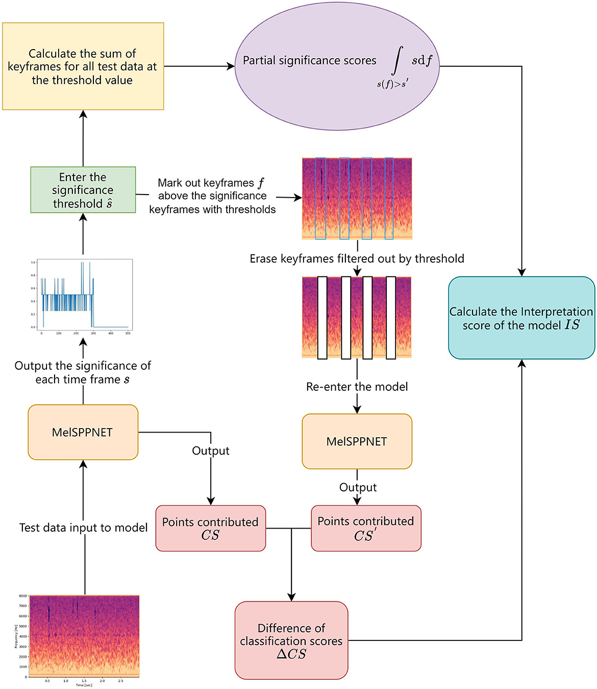
Figure 8. Interpretation score calculation process.

4 Experimental results and analysis

4.1 Experimental environment

This institute utilized environment equipment such as Intel(R) Xeon(R) Platinum 8255C 12 vCPU (43GB memory) and GeForce GTX 3080 (10GB VRAM), and was implemented using the PyTorch deep learning framework. The hyperparameters were set through manual tuning and automatic tuning methods. Based on the related experiments in audio recognition and the workload of this study, we manually adjusted the hyperparameters. After a large number of experiments, we found the best-performing parameter sizes and used them. The batch size was set to 512, and the model training ended after 12 epochs.

4.2 Experimental results

4.2.1 Accuracy of recognition

The identification of EAB is performed on a single audio basis, and the accuracy of audio recognition is used as the final evaluation metric for the models. To compare the recognition performance of various networks, pre-processing of the test audio is required before inputting it into the network model, as described in Section 3.1.2, where the log Mel-spectrogram features are converted to one-dimensional data for input. This process is a fundamental step in audio recognition and is independent of the choice of recognition method.

To verify the recognition accuracy of MelSPPNET, we conducted comparative experiments with several established network structures. In convolutional neural networks, as the number of layers increases, their ability to adapt to more complex functions also increases. However, for vibration signal recognition, a relatively simple network structure can achieve high accuracy (Grezmak et al., 2019). Therefore, in our experiments, we used traditional CNN networks as the basic convolutional layers of MelSPPNET and modified them to be suitable for one-dimensional data, training them with the same hyperparameters. We used ResNet-18, ResNet-34, VGG-16, and VGG-19 with a few layers as the basic convolutional layers for MelSPPNET and ResNet-18, ResNet-34, VGG-16, and VGG-19 without the prototype layer as the baseline models for comparison of accuracy. We chose ResNet network because its structure includes residual blocks, which can avoid the problems of vanishing or exploding gradients and has fewer parameters, resulting in faster training speed. We chose VGG network because it has a simple structure, is easy to understand and implement, and has high accuracy.

As shown in Table 2, the experimental results indicate that the introduction of the prototype layer did not have a negative impact on the accuracy of MelSPPNET. Moreover, the influence on recognition accuracy is correlated with the recognition accuracy of the backbone network.

Table 2

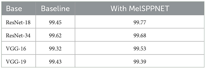
Table 2. Recognition accuracy comparison.

4.2.2 Reliability of the interpretation

We applied the interpretability evaluation metric we designed to evaluate the interpretability of MelSPPNET (with ResNet-18 as the backbone network) by inputting saliency threshold values ranging from 0.3 to 0.99 in steps of 0.01, and calculated the Interpretation score IS using the method described in Section 3.6. We listed the IS of the top 10 test data in Table 3.

Table 3

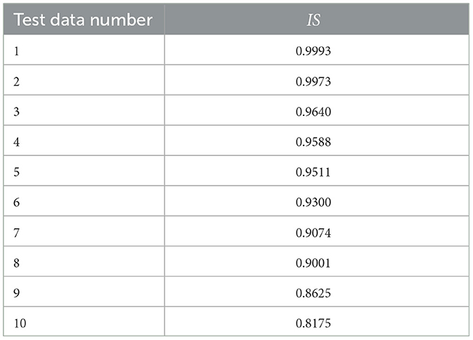
Table 3. Top 10 test data with interpretation score of MelSPPNET.

From the table, we can see that an IS > 0.8 indicates a high correlation between the significance score and classification score difference, indicating a high interpretability of our MelSPPNET. This suggests that our model has indeed extracted the vibration signal segments in the EAB larval feeding sound as intended and used them as the basis for Recognition of input data.

5 Discussion

In the process of detecting target tree trunk signals, it is necessary to first embed a ceramic piezoelectric sensor with a probe into the target tree trunk, then record the vibration signal and input it into MelSPPNET. MelSPPNET compares the input vibration signal with the existing prototype, and finally provides classification results.

In the context of EAB vibration signal recognition, MelSPPNET utilizes a methodology akin to human cognition. It leverages the existing “knowledge” acquired during training to seek diverse pieces of evidence and subsequently compares them with novel, unseen data. This comparative analysis aims to identify the most salient features of the input data and facilitate informed decision-making. This paradigm is especially well-suited for structured vibration signals that exhibit discernible patterns and do not necessitate substantial temporal dependencies.

In the actual execution process, the feeding vibration of EAB is accompanied by its own displacement, and the distance range of the feeding vibration signal that the sensor can sense is limited, which is determined by the physical properties of signal propagation. Therefore, in subsequent research, simultaneous detection of different positions of the same wood segment is also crucial.

In Section 4.2, not all data achieved a high IS, and we believe this is due to the inevitable influence of systematic environmental noise during data collection, such as the chirping of cicadas during field sampling. The environmental noise introduced contains regular patterns that affect the extraction of prototypes from the audio segments. To achieve higher IS and more accurate prototypes, it is necessary to perform pre-processing denoising on the collected data and the data to be identified before inputting it into the model. This is because the features of the burrowing vibration signals we need to identify are fixed, but the environmental noise that may be collected can vary significantly.

In terms of potential use, in terms of pest management, some studies have shown that there may be multiple stem borers for the same tree species, and different stem borers require different management methods. Therefore, classification of stem borers is also an important research direction. In theory, if two different stem borers produce different frequencies of feeding vibration signals due to their body size, MelSPPNET can be used to distinguish them; In terms of the prevention and control of invasive alien species, it is worth exploring whether changes in the shape of wood after processing into industrial products or during transportation as wood segments will result in different vibration signals of dry boring pests.

We attempted to use MelSPPNET for traditional sound signal recognition on the Urbansound8k dataset, but the network's recognition performance was not satisfactory. The reason for this may be that sound signals, unlike vibration signals, do not have periodic regularity, the training data did not undergo data augmentation and contained relatively high levels of noise, and there were similar and easily confused classes among different categories. As a result, MelSPPNET could not extract widely applicable prototypes for each class, thus failing to achieve high accuracy.

6 Conclusions

In this study, we proposed a case-based SEM MelSPPNET for the accurate and reliable identification of EAB feeding vibration signals collected using a piezoelectric ceramic sensor, while generating human-understandable prototypes. We also proposed an interpretable evaluation index IS for the case-based SEM, which can be used to evaluate an SEM. By strengthening the diversity and credibility of the prototypes through the loss function, our proposed method can adapt to the monitoring tasks of forest EAB and provide technical support for automatic monitoring and early warning identification of EAB in forests. Moreover, the human-understandable prototypes extracted by our model reduce the learning threshold for EAB recognition among forest pest monitoring personnel.

In the process of data collection, due to the lack of certain knowledge regarding larval stage and density of EAB, we focused solely on using MelSPPNET to identify the vibrational signal features of EAB larvae. We did not consider potential differences in vibrational signals that could arise from variations in larval stage and density within the trees. Additionally, since our measurements were taken during the growth phase of new larvae, there might be subtle changes in vibration signals as the larvae mature over time. The growth of trees with changing dates might also have some impact on vibration signals. However, we believe that the vibrational signals used to determine the presence of EAB larvae exhibit generally consistent features across different larval stages. In future data collection efforts, we will verify this assumption if we obtain EAB vibrational signals from different time periods.

In future work, if more pest feeding vibration signals or other regular industry vibration signals can be collected, we will improve our model and extend it to the reliable identification of more types of vibration signals.

Data availability statement

The raw data supporting the conclusions of this article will be made available by the authors, without undue reservation.

Author contributions

WJ: conceptualization, methodology, validation, formal analysis, investigation, resources, writing—original draft preparation, visualization, supervision, and writing—review and editing. ZC: conceptualization, methodology, validation, formal analysis, investigation, resources, writing—original draft preparation, supervision, project administration, and funding acquisition. HZ: conceptualization, methodology, validation, formal analysis, investigation, resources, writing—original draft preparation, supervision, and project administration. JL: conceptualization, methodology, validation, formal analysis, investigation, resources, writing—original draft preparation, and supervision. All authors contributed to the article and approved the submitted version.

Funding

This work was supported by The National Natural Science Foundation of China [grant number 32071775]. Beijing Forestry University Forestry First Class Discipline Construction Project [grant number 450-GK112301042]. They have agreed to pay the publication fees pending review and acceptance of the manuscript.

Acknowledgments

We would like to thank the authors who jointly completed the article and the peer reviewers for their valuable contributions to this research.

Conflict of interest

The authors declare that the research was conducted in the absence of any commercial or financial relationships that could be construed as a potential conflict of interest.

Publisher's note

All claims expressed in this article are solely those of the authors and do not necessarily represent those of their affiliated organizations, or those of the publisher, the editors and the reviewers. Any product that may be evaluated in this article, or claim that may be made by its manufacturer, is not guaranteed or endorsed by the publisher.

References

Cai, G., Li, J., Liu, X., Chen, Z., and Zhang, H. (2023). Learning and compressing: low-rank matrix factorization for deep neural network compression. Appl. Sci. 13:2704. doi: 10.3390/app13042704

Crossref Full Text | Google Scholar

Chen, C., Li, O., Tao, D., Barnett, A., Rudin, C., and Su, J. K. (2019). This looks like that: deep learning for interpretable image recognition. Adv. Neural Inf. Process. Syst. 32. doi: 10.48550/arXiv.1806.10574

Crossref Full Text | Google Scholar

Davydenko, K., Skrylnyk, Y., Borysenko, O., Menkis, A., Vysotska, N., Meshkova, V., et al. (2022). Invasion of emerald ash borer agrilus planipennis and ash dieback pathogen hymenoscyphus fraxineus in ukraine—a concerted action. Forests 13:789. doi: 10.3390/f13050789

Crossref Full Text | Google Scholar

DeGrave, A. J., Janizek, J. D., and Lee, S.-I. (2021). Ai for radiographic covid-19 detection selects shortcuts over signal. Nat. Mach. Intell. 3, 610–619. doi: 10.1038/s42256-021-00338-7

Crossref Full Text | Google Scholar

Donnelly, J., Barnett, A. J., and Chen, C. (2022). “Deformable protopnet: an interpretable image classifier using deformable prototypes,” in Proceedings of the IEEE/CVF Conference on Computer Vision and Pattern Recognition, 10265–10275.

Google Scholar

Du, D. (2019). Research on Acoustic Information Characteristics and Automatic Identification of Blueberry Typical Pests(in Chinese) (Master's thesis). Guizhou University, Guiyang, China.

Google Scholar

Gautam, S., Höhne, M. M.-C., Hansen, S., Jenssen, R., and Kampffmeyer, M. (2022b). “Demonstrating the risk of imbalanced datasets in chest x-ray image-based diagnostics by prototypical relevance propagation,” in 2022 IEEE 19th International Symposium on Biomedical Imaging (ISBI) (IEEE), 1–5.

Google Scholar

Gautam, S., Boubekki, A., Hansen, S., Salahuddin, S. A., Jenssen, R., Höhne, M., et al. (2022a). Protovae: a trustworthy self-explainable prototypical variational model. arXiv [preprint]. doi: 10.48550/arXiv.2210.08151

Crossref Full Text | Google Scholar

Grezmak, J., Zhang, J., Wang, P., Loparo, K. A., and Gao, R. X. (2019). Interpretable convolutional neural network through layer-wise relevance propagation for machine fault diagnosis. IEEE Sens. J. 20, 3172–3181. doi: 10.1109/JSEN.2019.2958787

Crossref Full Text | Google Scholar

Inyang, E. I., Hix, R. L., Tsolova, V., Rohde, B. B., Dosunmu, O., and Mankin, R. W. (2019). Subterranean acoustic activity patterns of vitacea polistiformis (lepidoptera: Sesiidae) in relation to abiotic and biotic factors. Insects 10, 267. doi: 10.3390/insects10090267

PubMed Abstract | Crossref Full Text | Google Scholar

Jiang, Q., Liu, Y., Ren, L., Sun, Y., and Luo, Y. (2022). Acoustic detection of the wood borer, semanotus bifasciatus, as an early monitoring technology. Pest Manag. Sci. 78, 4689–4699. doi: 10.1002/ps.7089

PubMed Abstract | Crossref Full Text | Google Scholar

Kahl, S., Wilhelm-Stein, T., Klinck, H., Kowerko, D., and Eibl, M. (2018). “A baseline for large-scale bird species identification in field recordings,” in CLEF (Working Notes), 2125.

Google Scholar

Kim, E., Kim, S., Seo, M., and Yoon, S. (2021). “Xprotonet: diagnosis in chest radiography with global and local explanations,” in Proceedings of the IEEE/CVF Conference on Computer Vision and Pattern Recognition, 15719–15728.

Google Scholar

Kovacs, K. F., Haight, R. G., McCullough, D. G., Mercader, R. J., Siegert, N. W., and Liebhold, A. M. (2010). Cost of potential emerald ash borer damage in us communities, 2009-2019. Ecol. Econ. 69, 569–578. doi: 10.1016/j.ecolecon.2009.09.004

Crossref Full Text | Google Scholar

Liu, X., Zhang, H., Jiang, Q., Ren, L., Chen, Z., Luo, Y., et al. (2022). Acoustic denoising using artificial intelligence for wood-boring pests semanotus bifasciatus larvae early monitoring. Sensors 22:3861. doi: 10.3390/s22103861

PubMed Abstract | Crossref Full Text | Google Scholar

Liu, X., Sun, Y., Cui, J., Jiang, Q., Chen, Z., and Luo, Y. (2021). Early recognition of feeding sound of trunk borers based on artifical intelligence. Sci. Silvae Sin 57, 93–101. doi: 10.11707/j.1001-7488.20211009

Crossref Full Text | Google Scholar

Lundberg, S. M., and Lee, S.-I. (2017). A unified approach to interpreting model predictions. Adv. Neural Inf. Process. Syst. 30, 4765–4774. doi: 10.48550/arXiv.1705.07874

Crossref Full Text | Google Scholar

Luo, C.-Y., Pearson, P., Xu, G., and Rich, S. M. (2022). A computer vision-based approach for tick identification using deep learning models. Insects 13:116. doi: 10.3390/insects13020116

PubMed Abstract | Crossref Full Text | Google Scholar

MacFarlane, D. W., and Meyer, S. P. (2005). Characteristics and distribution of potential ash tree hosts for emerald ash borer. For. Ecol. Manage. 213, 15–24. doi: 10.1016/j.foreco.2005.03.013

Crossref Full Text | Google Scholar

McCullough, D., and Katovich, S. (2004). Pest alert: emerald ash borer. United States Forest Service, Northeastern Area. Technical Report.

Google Scholar

Murfitt, J., He, Y., Yang, J., Mui, A., and De Mille, K. (2016). Ash decline assessment in emerald ash borer infested natural forests using high spatial resolution images. Remote Sens. 8:256. doi: 10.3390/rs8030256

Crossref Full Text | Google Scholar

Mwangola, D. M., Kees, A. M., Grosman, D. M., and Aukema, B. H. (2022). Effects of systemic insecticides against emerald ash borer on ash seed resources. For. Ecol. Manage. 511:120144. doi: 10.1016/j.foreco.2022.120144

Crossref Full Text | Google Scholar

Omeiza, D., Webb, H., Jirotka, M., and Kunze, L. (2021). Explanations in autonomous driving: a survey. IEEE Transact. Intell. Transport. Syst. 23, 10142–10162. doi: 10.1109/TITS.2021.3122865

Crossref Full Text | Google Scholar

Poland, T. M., and McCullough, D. G. (2006). Emerald ash borer: invasion of the urban forest and the threat to North America's ash resource. J. Forest. 104, 118–124. doi: 10.1093/jof/104.3.118

Crossref Full Text | Google Scholar

Ribeiro, M. T., Singh, S., and Guestrin, C. (2016). ““Why should i trust you?” explaining the predictions of any classifier,” in Proceedings of the 22nd ACM SIGKDD International Conference on Knowledge Discovery and Data Mining, 1135–1144. doi: 10.1145/2939672.2939778

Crossref Full Text | Google Scholar

Rudin, C. (2019). Stop explaining black box machine learning models for high stakes decisions and use interpretable models instead. Nat. Mach. Intell. 1, 206–215. doi: 10.1038/s42256-019-0048-x

PubMed Abstract | Crossref Full Text | Google Scholar

Rutledge, C. E. (2020). Preliminary studies on using emerald ash borer (coleoptera: Buprestidae) monitoring tools for bronze birch borer (coleoptera: Buprestidae) detection and management. Forestry 93, 297–304. doi: 10.1093/forestry/cpz012

Crossref Full Text | Google Scholar

Shah, R., Dave, B., Parekh, N., and Srivastava, K. (2022). “Parkinson's disease detection-an interpretable approach to temporal audio classification,” in 2022 IEEE 3rd Global Conference for Advancement in Technology (GCAT) (IEEE), 1–6. doi: 10.1109/GCAT55367.2022.9971881

Crossref Full Text | Google Scholar

Shi, H., Chen, Z., Zhang, H., Li, J., Liu, X., Ren, L., et al. (2022). A waveform mapping-based approach for enhancement of trunk borers' vibration signals using deep learning model. Insects 13:596. doi: 10.3390/insects13070596

PubMed Abstract | Crossref Full Text | Google Scholar

Sun, Y., Tuo, X., Jiang, Q., Zhang, H., Chen, Z., Zong, S., et al. (2020). Drilling vibration identification technique of two pest based on lightweight neural networks. Sci. Silvae Sin 56, 100–108. doi: 10.11707/j.1001-7488.20200311

Crossref Full Text | Google Scholar

Sutin, A., Yakubovskiy, A., Salloum, H. R., Flynn, T. J., Sedunov, N., and Nadel, H. (2019). Towards an automated acoustic detection algorithm for wood-boring beetle larvae (coleoptera: Cerambycidae and buprestidae). J. Econ. Entomol. 112, 1327–1336. doi: 10.1093/jee/toz016

PubMed Abstract | Crossref Full Text | Google Scholar

Wang, B., Mao, Y., Ashry, I., Al-Fehaid, Y., Al-Shawaf, A., Ng, T. K., et al. (2021). Towards detecting red palm weevil using machine learning and fiber optic distributed acoustic sensing. Sensors 21:1592. doi: 10.3390/s21051592

PubMed Abstract | Crossref Full Text | Google Scholar

Wang, J., Liu, H., Wang, X., and Jing, L. (2021). “Interpretable image recognition by constructing transparent embedding space,” in Proceedings of the IEEE/CVF International Conference on Computer Vision, 895–904. doi: 10.1109/ICCV48922.2021.00093

Crossref Full Text | Google Scholar

Ward, S. F., Liebhold, A. M., Morin, R. S., and Fei, S. (2021). Population dynamics of ash across the eastern usa following invasion by emerald ash borer. For. Ecol. Manage. 479:118574. doi: 10.1016/j.foreco.2020.118574

Crossref Full Text | Google Scholar

Zhou, Q., Yu, L., Zhang, X., Liu, Y., Zhan, Z., Ren, L., et al. (2022). Fusion of uav hyperspectral imaging and lidar for the early detection of eab stress in ash and a new eab detection index—ndvi (776,678). Remote Sens. 14:2428. doi: 10.3390/rs14102428

Crossref Full Text | Google Scholar

Zhou, B., Khosla, A., Lapedriza, A., Oliva, A., and Torralba, A. (2016). “Learning deep features for discriminative localization,” in Proceedings of the IEEE Conference on Computer Vision and Pattern Recognition, 2921–2929.

Google Scholar

Zhu, L., and Zhang, Z. (2012). Automatic recognition of insect sounds using mfcc and gmm. Acta Entomol. Sin. 55, 466–471. Available online at: http://www.insect.org.cn/CN/abstract/article_5111.shtml

Google Scholar