Depth-Dependent Correction for Wind-Driven Drift Current in Particle Tracking Applications

1. Introduction

It is important to predict the trajectories of buoyant objects at the ocean surface for a wide variety of applications, such as: search and rescue purposes (e.g., Breivik and Allen, 2008); oil spill mitigation (e.g., Abascal et al., 2009b; le Hénaff et al., 2012); tracking of marine plastic debris (e.g., Lebreton et al., 2012); and determining larval (e.g., Siegel et al., 2003) or seed dispersal (e.g., Erftemeijer et al., 2008). Trajectories of buoyant objects are commonly simulated using Lagrangian particle tracking models (PTMs). However, many uncertainties are involved in particle tracking simulations (PTSs) (e.g., van Sebille et al., 2018), for example: unresolved processes in the forcing fields used to advect particles; inaccuracy in numerical solvers of PTMs; and uncertainty about the dynamics of objects at the ocean surface. Specifically, uncertainty about relevant transport mechanisms (e.g., currents, wind, waves) can lead to large errors (e.g., le Hénaff et al., 2012; van der Mheen et al., 2019).

In addition to “background surface currents” (section 2) used to force PTMs, wind has a large impact on the transport of buoyant objects, both directly and indirectly. Directly, an object protruding from the ocean surface is influenced by wind forcing or windage (e.g., Breivik et al., 2011), acting on the surface area exposed to air. Indirectly, wind generates a surface “drift current.” Wu (1983) suggested that the drift current consists of two components: (1) wind-induced shear current, and (2) wave-induced Lagrangian Stokes drift (e.g., van den Bremer and Breivik, 2017). Waves are generated by wind both remotely (“swell”) and locally (“sea”), but sea waves contribute most to Stokes drift (Clarke and van Gorder, 2018). Both the total drift current and Stokes drift have been studied extensively, sometimes leading to contradictory results, as described in the following paragraphs.

Results are inconsistent regarding the relative contribution of the wind-induced shear current and Stokes drift on the total drift current. The drift current at the ocean surface is generally estimated at roughly 3% of the wind speed (at 10-m height) (e.g., Hughes, 1956). Wu (1983) showed that Stokes drift makes up two thirds (roughly 2% of the wind speed) of the surface drift current. In contrast, more recent studies estimate lower values for surface Stokes drift: roughly 1% of the wind speed (e.g., Ardhuin et al., 2009; Clarke and van Gorder, 2018). Despite this, these studies focus primarily on Stokes drift rather than the total drift current.

There are also inconsistencies in the angle of the drift current compared to the wind. Classical Ekman theory (Ekman, 1905) predicts that the wind-driven surface current is rotated 45° to the right of the wind in the northern hemisphere and to the left in the southern hemisphere. In contrast, Madsen (1977) predicted a surface deflection of 10° to the wind. Observations show a wide variety of deflection angles, ranging anywhere between 0° (Hughes, 1956) and 90° (Ardhuin et al., 2009).

Finally, there is no consensus about the drift current's vertical structure. Traditionally, the drift current was suggested to follow a logarithmic vertical profile (e.g., Richman et al., 1987), much like the vertical profile of the wind close to a boundary (e.g., Tennekes, 1972). However, Stokes drift decays exponentially with depth (e.g., van den Bremer and Breivik, 2017) and little is known about the vertical profile of the wind-induced shear current. Some studies indicate that this profile is relatively uniform with depth (e.g., Ardhuin et al., 2009), whereas others show evidence of a strong vertical gradient (Morey et al., 2018), particularly in the top few centimeters of the water column (Laxague et al., 2017). Regardless of the precise vertical structure, it is accepted that the drift current has a strongly decaying vertical profile, which can have a large impact on the transport of buoyant objects. However, few studies give practical suggestions how to account for the vertical profile of the drift current in particle tracking applications (PTAs).

To simulate oil spills, 3% of the wind speed is commonly added to background currents to account for the surface drift current (e.g., le Hénaff et al., 2012). Similar practices are used to simulate dispersion of seagrass seeds (e.g., Erftemeijer et al., 2008). However, modern ocean circulation models have higher vertical resolution than models for which these drift current corrections were designed. In addition, other sources of surface currents, such as high-frequency radar (HFR) measurements, may already contain the wind-induced shear current (Hammond et al., 1987) and Stokes drift (Chavanne, 2018). It is therefore unclear if a drift current correction is still needed in PTAs, and, if so, what the best way is to incorporate it. This question was also raised by Morey et al. (2018) and Haza et al. (2019).

Morey et al. (2018) found significant differences between HFR measured current velocities and velocities in the upper few centimeters of the ocean surface layer, indicating that a drift current correction is still relevant to simulate surface transport using HFR currents. Haza et al. (2019) simulated trajectories of ocean surface drifters based on currents from a state-of-the-art ocean circulation model and by adding wind and wave data using different methods. Essentially, they calibrated the drift current correction to best fit specific current, wind, and wave datasets to predict drifter trajectories. However, for most applications, calibrating PTMs with trajectory data is an unavailable luxury. In these cases, a more general rule of thumb to account for the drift current is useful.

The aim of this paper is to illustrate the importance of the vertical profile of the drift current on the transport of buoyant objects, and to emphasize that this should be accounted for in PTAs. We introduce a depth-dependent drift current correction factor (“drift factor,” section 2) that is straightforward to apply to PTSs. We test the usefulness of the drift factor by applying it to simulations of the transport of two types of ocean surface drifters that we released simultaneously in an HFR field.

Our results show that the two types of drifters behave differently, which we suggest is related to the vertical decay of the wind-driven drift current. Our PTS results provide an illustrative example, indicating the importance of accounting for the drift current and the usefulness of the drift factor.

2. Drift Factor

The drift current is a wind-induced ocean surface current. However, the definition of a “surface” current is ambiguous (Laxague et al., 2017). We follow the distinction of Fernández et al. (1996), separating surface currents into three regions: (1) A region immediately below the air-sea interface of several millimeters thick that is dominated by viscous effects. (2) A region where the velocity varies logarithmically with depth, varying from its surface value of roughly 3% of the wind speed, to an upper Ekman layer value. (3) The Ekman layer.

We are interested only in layer (2). In this layer, the ocean current consists of: geostrophic currents, tidal currents, assorted baroclinic currents, Stokes drift, and wind-induced shear currents (Fernández et al., 1996). Following Laxague et al. (2017), we refer to geostrophic, tidal, and baroclinic currents as “background currents.” Stokes drift and the wind-induced shear current together make up the wind-driven “drift current” (Wu, 1983).

The drift current responds to instantaneous changes in the wind field. These changes are generally on much shorter timescales than the inertial period, so the drift current should be unaffected by the Coriolis force (Fernández et al., 1996). As a result, the drift current is directed downwind. In the distinction of Fernández et al. (1996), the Coriolis force affects currents in layer (3), where they are deflected according to Ekman theory.

Stokes drift is a Lagrangian current, mostly due to locally generated sea waves, even in the presence of large swell waves (Clarke and van Gorder, 2018). The Coriolis-Stokes force induces a Eulerian current which can cancel out Stokes drift (Hasselmann, 1970). However, this is negligible if the Stokes drift vertical decay scale is smaller than that of the Ekman layer (Clarke and van Gorder, 2018). Since this is generally the case in the open ocean, Stokes drift is likely an important component of the drift current.

Because both Stokes drift and the wind-induced shear current are wind-driven, they are difficult to separate. We therefore consider the total effect of the drift current ${\overrightarrow{u}}_{drift}$ and assume it has a logarithmic vertical profile (e.g., Pugh, 1987; Chavanne, 2018):

$\begin{array}{ll}{\overrightarrow{u}}_{drift}(z)={\overrightarrow{u}}_0-\frac{{\overrightarrow{u}}_{*}}{\kappa }log\left(\frac{z}{z_0}\right).& (1)\end{array}$

Here, ${\overrightarrow{u}}_0$ is the surface drift current; ${\overrightarrow{u}}_{*}=\sqrt{\frac{\overrightarrow{\tau }}{{\rho }_w}}$ the friction current, with wind stress $\overrightarrow{\tau }={\rho }_a{C}_D{\overrightarrow{u}}_{10}^2$, C_D the drag coefficient, ρ_a and ρ_w the density of air and sea water, respectively, ${\overrightarrow{u}}_{10}$ the wind field at 10 m height; κ = 0.41 von Karman's constant; z₀ the roughness length on the ocean side (which may differ from that on the atmosphere side, Wu, 1983); and z the depth.

We can rewrite Equation (1) as a simple function of the wind field,

$\begin{array}{ll}{\overrightarrow{u}}_{drift}(z)=\left[\alpha -\beta log\left(\frac{z}{z_0}\right)\right]·{\overrightarrow{u}}_{10}=R(z)·{\overrightarrow{u}}_{10},& (2)\end{array}$

with α = 0.03 and β≈0.0027; assuming that ${\overrightarrow{u}}_0=0.03·{\overrightarrow{u}}_{10}$, ρ_a = 1.2 kg/m³, ρ_w = 1025 kg/m³, and C_D = 0.00104 (for wind speeds under 7 m/s, Amorocho and DeVries, 1980). Following Pugh (1987), we assume a small value of z₀ = −0.001 m, which prevents singularities at z = 0.

The parameter R(z) in Equation (2) is the depth-dependent drift current correction factor, or “drift factor.” If we assume that the total current field $\overrightarrow{u}$ at depth z is given by

$\begin{array}{ll}\overrightarrow{u}(z)={\overrightarrow{u}}_{background}+{\overrightarrow{u}}_{drift}(z),& (3)\end{array}$

and that current fields in PTSs represent background currents ${\overrightarrow{u}}_{background}$, it is then straightforward to correct ${\overrightarrow{u}}_{background}$ for the drift current:

$\begin{array}{ll}\overrightarrow{u}(z)={\overrightarrow{u}}_{background}+R(z)·{\overrightarrow{u}}_{10}.& (4)\end{array}$

We apply this correction to two types of ocean surface drifters, and determine the effect on PTSs.

3. Methodology

3.1. Drifter Experiment and Datasets

3.1.1. Ocean Surface Drifters

We simultaneously released 4 undrogued and 4 drogued drifters off the Rottnest Shelf in Western Australia (Figure 1A) on 27-04-2017 around 05:15 UTC. Both types of drifters consist of a cylindrical PVC housing containing ballast weight, batteries, and a SPOT Trace^TM device which transmits locations every 5-min through the GlobalStar® network (Figure 1B). The drogued drifters have an Oceansouth sea anchor.

FIGURE 1

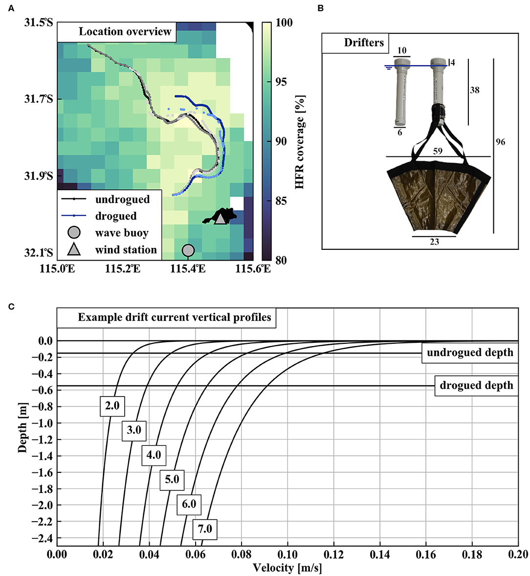
Figure 1. (A) Overview showing: tracks of three undrogued and two drogued drifters for 5 days after release; HFR coverage of good quality data for 5 days after drifter release; locations of Bureau of Meteorology Rottnest Island wind station and Department of Transport wave buoy. (B) Photo of undrogued and drogued drifters with sizes indicated in centimeters (rounded up to whole centimeters). (C) Schematic showing: example vertical profiles of the logarithmic drift current for different wind speeds (numbers in text boxes for each profile indicate ${\overrightarrow{u}}_{10}$ speeds in m/s); representative depths of the undrogued and drogued drifters.

Both drifter designs have a low area exposed to air (blue line in Figure 1B indicates approximate water level), so we assume that windage on both drifters is negligible. We further assume that undrogued drifters represent currents at approximately z_ud = −0.15 m (roughly half the submerged depth of the drifter) and drogued drifters at z_dd = −0.50 m (roughly the depth at which the sea anchor is centered when it opens and trails behind the moving drifter). Example logarithmic profiles in Figure 1C illustrate how the drift current varies with depth for different wind speeds.

One undrogued and two drogued drifters failed prematurely or transmitted too sparsely, so we only use locations from 3 undrogued and 2 drogued drifters. We quality control the drifter locations following Hansen and Poulain (1996) (Figure S1). We then interpolate locations to regular time intervals of 10 min, marking gaps between locations of more than 20 min as missing data. We calculate drifter velocities using a central differencing scheme. For comparison with HFR measured currents (section 3.1.2) we calculate hourly averaged drifter velocities.

Several other studies used SPOT Trace^TM devices in drifters (e.g., Morey et al., 2018; Pawlowicz et al., 2019). Morey et al. (2018) reported a standard error under calm sea conditions of approximately 4 m in positioning. These errors are negligible for the purpose of this paper.

3.1.2. High-Frequency Radar (HFR) Measured Current Field

We deployed drifters on 27-04-2017 in a region where an HFR system measures surface currents using shore-based Wellen Radars (WERA) transmitting at 9.33 MHz frequency (Cosoli et al., 2018). After processing and quality control, hourly averaged currents with horizontal resolution of 4 km are available. Good quality HFR coverage of the area was available during the drifter experiment (Figure 1A).

The HFR system emits radio waves with wavelength λ. These are backscattered off the ocean surface at ${\lambda }_B=\frac{\lambda }{2}$, with λ_B the Bragg wavelength (e.g., Ivonin, 2004). Current velocities are determined using the Doppler shift of Bragg waves. The frequency f of the WERA system corresponds to a Bragg wavelength of ${\lambda }_B=\frac{c}{2f}\approx 16.1$ m, with c the speed of light. HFR systems are assumed to measure currents up to a depth of $z=-\frac{{\lambda }_B}{4\pi }$. This corresponds to z≈−1.3 m for the WERA system, and measurements can be roughly interpreted as depth-averaged currents to 1.3 m depth.

Although there is still controversy (e.g., Rohrs et al., 2015), it seems that HFR systems also measure depth-averaged Stokes drift (Chavanne, 2018). However, to keep application of the drift factor simple, we correct HFR measured currents following Equation (4). If HFR indeed measures Stokes drift as well as background currents, we may be over-correcting for the drift current (which consists in part of Stokes drift).

We use HFR currents as forcing fields for PTSs (section 3.3) as well as for direct comparison with drifter velocities. To make this comparison, we linearly interpolate HFR currents to the mean drifter track (Figure S2).

3.1.3. Wind Data

An Australian Government Bureau of Meteorology station on Rottnest Island (Figure 1A) measures wind speed and direction at 43.1m height every 30 min. We converted these measurements to standard 10m reference height (Figure S3), and use hourly averages for comparisons with drifter and HFR velocities.

We validated an operational WRF-model (www.coastaloceanography.org) to consider spatial variations in the wind field during the drifter experiment (Figure S4). The WRF simulated wind is very similar at Rottnest Island and along the mean drifter track. It is therefore justified to use measured wind at Rottnest for comparison with drifter velocities. We also use hourly averaged wind at Rottnest as forcing for PTSs.

3.1.4. Wave Data

A Western Australian Government Department of Transport (DoT) Datawell wave buoy to the southwest of Rottnest Island (Figure 1A) samples vertical displacement of the sea surface with a frequency of 1.28 Hz (Government of Western Australia Department for Planning and Infrastructure, 2009). DoT provides significant wave heights, peak periods, and directions for swell and sea waves every 20 min (Figure S5a).

Using this data, we estimated wavelengths (Figure S5b) and Stokes drift (Figure S5c). During the drifter experiment, Stokes drift from both swell and sea waves is mostly negligible. However, as sea wave peak period drops from roughly 5 to 3 s, Stokes drift becomes significant. These short periods are very close to the sampling frequency and barely satisfy the Nyquist criterion, so we cannot be sure about the accuracy of these measurements. We therefore do not consider Stokes drift separately in this paper, but instead focus on the overall effect of the drift current. In this case, it is reasonable to consider the Stokes drift implicitly as a function of the wind, because Stokes drift due to swell waves is negligible during the drifter experiment (Figure S5c), and any Stokes drift due to locally generated sea waves will be aligned with the wind.

3.2. Velocity Comparisons

To determine if the behavior of the two types of drifters is different, we compare their velocities. We also compare them to HFR currents and winds.

After 5 days, undrogued and drogued drifter tracks have clearly separated (Figure 1A). However, this does not necessarily mean that the behavior of the two types of drifters is significantly different. A small change in a drifter's location can move it into a different current regime, which can amplify and lead to exponential separation (LaCasce, 2008). We see this effect in the daily tracks of undrogued and drogued drifters with an overlay of HFR current fields (Figures 2A–E): after day 1 undrogued and drogued drifters separate; from day 2 to 4 the distance slowly increases as undrogued drifters are influenced by different currents; and after day 5 undrogued drifters are swept up in an anticyclonic eddy and swiftly move away from the drogued drifters.

FIGURE 2

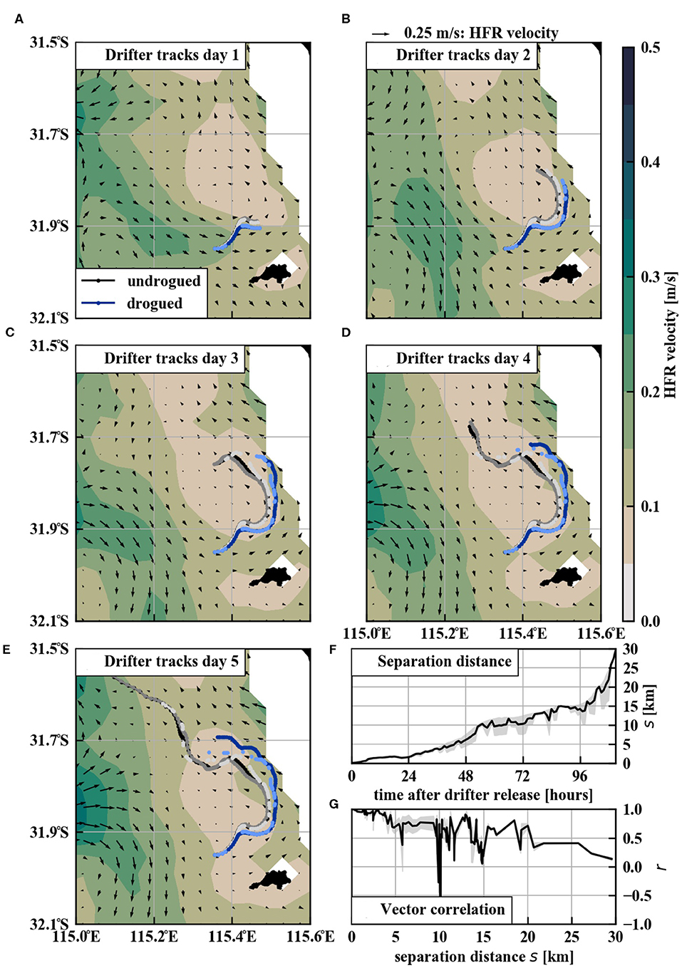
Figure 2. (A–E) Drifter tracks and daily mean HFR measured current field for the first 5 days after drifters release. (F) Mean separation distance s between undrogued and drogued drifters over time. Gray shading shows the minimum and maximum separation distance between an undrogued and drogued drifter. (G) Vector correlation magnitude r between undrogued and drogued drifters as a function of the separation distance. Following Rohrs et al. (2012) a vector correlation of 1 indicates perfect alignment of vectors, whereas −1 indicates perfect anti-alignment.

So, we can only compare velocities of undrogued and drogued drifters while they are transported by the same current field. The separation distance between the two drifter types increases over time (Figure 2F). As the separation distance increases, the vector correlation (e.g., Rohrs et al., 2012) decreases (Figure 2G). Within the first 24 h the separation distance remains well below 5 km and the vector correlation r is high, approaching r = 1.0. We are interested in a wind event in the first 15 h after drifter release (section 4.1). Both undrogued and drogued drifters are influenced by the same current field during this time, so a direct velocity comparison is justified.

3.3. Particle Tracking Simulations (PTSs)

We use OceanParcels-v2 (Lange and van Sebille, 2017; Delandmeter and van Sebille, 2019) to run 5 day PTSs of drifter transport, with a timestep of dt = 10 min. We choose 5 days because undrogued and drogued drifters are clearly separated after this time (Figure 2). We release 100 virtual particles at the drifter release location, adding Brownian particle diffusion with constant horizontal diffusion coefficient K_h = 10.0 m²/s. Simulating an ensemble of diffuse particles both ensures that particles spread out and sample different parts of the current field, and accounts for unresolved (turbulent) mixing processes. This is common practice in many PTAs (e.g., Peliz et al., 2007; le Hénaff et al., 2012).

We use HFR currents as forcing for PTSs, and use the drift factor R(z) Equation (2) to correct for the drift current at undrogued and drogued drifter depths. For undrogued drifters we find R(z_ud = −0.15m)≈0.02, and for drogued drifters R(z_dd = −0.50m)≈0.01. We run PTSs forced by HFR currents with: (1) no correction, as a baseline comparison; (2) a correction of $0.01·{\overrightarrow{u}}_{10}$, at drogued drifter depth; and (3) a correction of $0.02·{\overrightarrow{u}}_{10}$, at undrogued drifter depth. In addition, we run simulations with R = [0.005, 0.015, 0.025, 0.03] to compare simulation results for a range of different drift factors.

We use the mean cumulative separation distance D (e.g., Haza et al., 2019) as a quantitative measure of the performance of a PTS,

$\begin{array}{ll}D=\frac{1}{T·N}{\displaystyle \sum _{t=0}^T}{\displaystyle \sum _{i=1}^N}|{\overrightarrow{x}}_i(t)-{\overrightarrow{x}}_{obs}(t)|.& (5)\end{array}$

Here, ${\overrightarrow{x}}_i(t)$ is the location vector of a virtual particle i of a total of N particles, at time t for a total of T timesteps; and ${\overrightarrow{x}}_{obs}(t)$ is the corresponding drifter location.

4. Results

4.1. Velocity Comparisons

In the first 15 h after drifter release, the wind speed increases from roughly 2 to 7 m/s, and decreases again to 2 m/s. The downwind components of the HFR, drogued, and undrogued drifter velocities closely follow the increase and decrease in wind speed (Figure 3A, lower panel). The undrogued drifters have consistently larger velocities than drogued drifters, which in turn have larger velocity than the HFR currents. In contrast, the cross-wind components of the HFR, drogued, and undrogued drifter velocities are relatively similar, and drifter velocities are mostly within one standard deviation of the HFR currents (Figure 3A, upper panel). This is expected if drifters are transported by a wind-driven drift current that decays with depth.

FIGURE 3

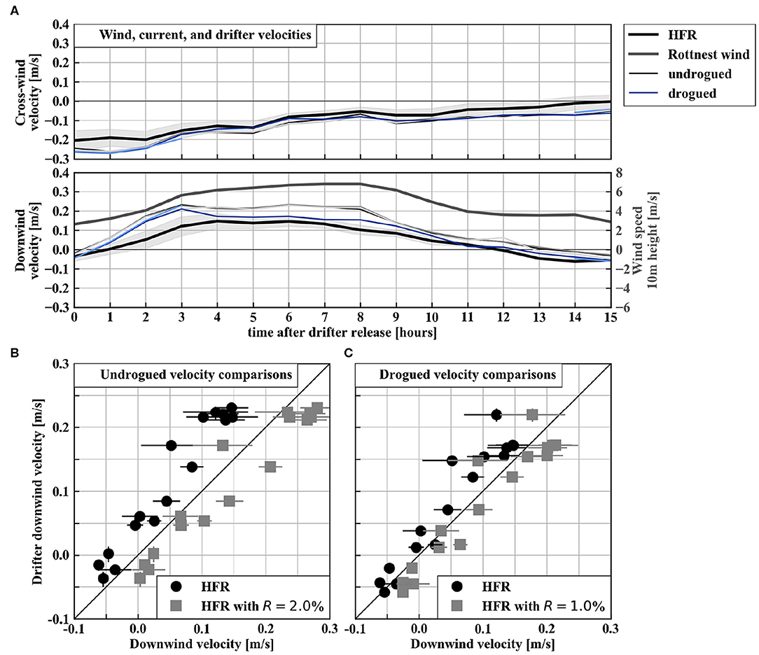
Figure 3. (A) Cross- and downwind components of: HFR measured velocity along the mean drifter track (shading shows HFR velocities plus and minus one standard deviation); measured wind speed at the Bureau of Meteorology (BoM) Rottnest wind station converted to a reference 10-m height; and velocities of three undrogued and two drogued drifters. (B) Downwind component comparisons of mean undrogued drifter velocities; uncorrected HFR measured currents; and HFR corrected currents with a drift factor of R = 0.02. (C) Downwind component comparisons of mean drogued drifter velocities; uncorrected HFR measured currents; and HFR corrected currents with a drift factor of R = 0.01. Horizontal bars in (B,C) show HFR velocity plus and minus one standard deviation. Vertical bars in (B,C) show minimum and maximum drifter velocities (where applicable).

For both undrogued and drogued drifters, the downwind HFR current components corrected with the drift factor match downwind drifter velocities better than uncorrected HFR currents (Figures 3B,C), although the drift factor slightly over-corrects current velocities. This indicates that HFR currents only may be insufficient to predict drifter transport, and that the vertical profile of the drift current should be taken into account in PTSs.

4.2. Particle Tracking Simulations (PTSs)

As suspected based on comparisons of drifter and HFR v-velocities, virtual particles forced only by HFR current fields do not extend as far north as either undrogued or drogued drifters (Figure 4A). In contrast, simulated particle trajectories forced by HFR currents corrected with a drift factor agree much better with the actual drogued (Figure 4B) and undrogued (Figure 4C) drifter trajectories. This is confirmed by the lower mean cumulative separation distances for these simulations (Figure 4 Table). The cumulative separation distances for PTS results with other values for the drift factor, also confirm that our estimates of R(z_ud) = 0.02 and R(z_dd) = 0.01 give the best PTS results, despite slightly over-correcting HFR currents (Figure 3C).

FIGURE 4

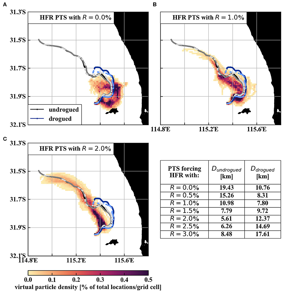
Figure 4. Particle density (percentage of particle locations per 0.01 × 0.01° grid cells) of 100 simulated virtual particles, until 5 days after release at the drifter deployment location. Particles are advected by HFR measured current fields with a drift current factor of: (A) R = 0.0; (B) R = 0.01 = 1.0%; (C) R = 0.02 = 2%; and include Brownian motion with constant horizontal diffusion coefficient K_h = 10.0. The trajectories of the undrogued (gray shades) and drogued (blue shades) drifters for 5 days after their release are also shown. (Table) Mean cumulative separation distance D between all 100 simulated virtual particles and an undrogued and drogued drifter for 5 days for simulations with different values for the drift factor.

5. Discussion

The aim of this paper is to emphasize the influence of the vertical profile of the wind-driven drift current on the transport of buoyant objects, and to introduce a straightforward drift factor, which is easy to apply to PTSs. Such a drift factor is particularly useful when no trajectory data is available to calibrate a PTM.

Comparison of velocities of undrogued drifters, drogued drifters, and HFR currents, shows a decreasing velocity with increasing depth. Similar results were also obtained by others (e.g., Morey et al., 2018). To explain this, most recent work focuses mainly on Stokes drift (e.g., Ardhuin et al., 2009; Clarke and van Gorder, 2018). However, Laxague et al. (2017) and Morey et al. (2018) showed that strong vertical decay cannot be explained by Stokes drift alone. We suggest that the wind-driven drift current is responsible for strong decay of velocities near the ocean surface. The drift current consists of both Stokes drift and a wind-induced shear current (Wu, 1983). This means that we cannot focus on Stokes drift alone, but need to take the full drift current into account.

We corrected for the drift current by using a drift factor R(z),

$\begin{array}{ll}\overrightarrow{u}(z)={\overrightarrow{u}}_{background}+{\overrightarrow{u}}_{drift}={\overrightarrow{u}}_{background}+R(z)·{\overrightarrow{u}}_{10},& (6)\end{array}$

$\begin{array}{ll}R(z)=\alpha -\beta \log \left(\frac{z}{z_0}\right).& (7)\end{array}$

We used values of α = 0.03, β = 0.0027, and z₀ = −0.001 m (section 2) to estimate drift factors for undrogued and drogued drifters. Our PTS results show that the drift factor improves simulation results. However, the drift factor is a first order estimate to account for the drift current. In addition, because the number of drifter locations that we use here is limited, our results should be interpreted as an illustrative example, highlighting the importance of the vertical profile of the drift current on the transport of buoyant objects, and emphasizing its potentially significant influence on PTS results.

We ignored effects of windage on the drifters. This is likely valid for drogued drifters, but less so for undrogued drifters. The windage coefficient R_windage is usually taken as (Richardson, 1997)

$\begin{array}{ll}{R}_{windage}=\sqrt{\frac{{\rho }_a}{{\rho }_w}\frac{C_{Da}}{C_{Dw}}\frac{A_a}{A_w}},& (8)\end{array}$

where ρ is the fluid density, C_D is the object's drag coefficient, A is the effective exposed area, and the subscripts a and w indicate parameters on the air and ocean side, respectively. For our undrogued drifters, the area ratio $\frac{A_a}{A_w}\approx 0.25$. Although questionable (Isobe et al., 2011), a drag coefficient ratio $\frac{C_{Da}}{C_{Dw}}=1.0$ is often assumed. Assuming $\frac{{\rho }_a}{{\rho }_w}=1.17·10^{-3}$, we get a windage coefficient for undrogued drifters of roughly 0.02, which is the same value that we found for the drift factor. It is possible to argue that it is not the drift current which influences undrogued drifters, but windage. However, with only about 4 cm protruding above the ocean surface, wind shear (which drives the drift current) is likely much more important than windage (which acts perpendicular to the protruding surface). Importantly, drogued drifters also have larger velocity than the HFR currents, which is not explained by windage, but is explained by the drift current. We therefore argue that the drift current, and not windage, is important for the transport of these drifters.

Several studies highlight the need for better understanding of the vertical profile of ocean surface currents (e.g., Morey et al., 2018). We also highlight the need for a method to account for the vertical current profile in PTAs, especially when no data is available to calibrate PTMs. The drift factor we introduced here is a first step toward this. It is straightforward in its application and improved PTS results in our case study. Further confirmation of this method, for example using larger drifter datasets and using HFR measured currents at different frequencies (and therefore different depths) as well as different state-of-the-art ocean models, is needed. In addition, we made assumptions for several parameter values, such as: the surface drift current velocity, which we assumed as 3% of the wind velocity; the drag coefficient; and the roughness length. Although these assumptions are based on commonly used values in the literature, they may not be optimal or valid under different conditions and need further investigation.

The aim of this paper was to determine drift factors without using trajectory data to calibrate a PTM. However, it is also possible to determine drift factors for the drogued and undrogued drifters using a best fit. This can be done by optimizing wind and current velocities to best match drifter velocities (e.g., Abascal et al., 2009a); or optimizing PTS results to best match drifter trajectories (e.g., Haza et al., 2019). These two methods do not necessarily result in the same values for a best fit. Using a best fit based on drifter velocities, we find R_ud = 0.013 and R_dd = 0.0063 for undrogued and drogued drifters, respectively (Figures S6a,b). These drift factors are significantly lower than those we determined using Equation (7) (R_ud = 0.02 and R_dd = 0.01). However, they do not improve PTS results (Figures S6c,d) compared to the drift factors determined using Equation (7) (Figure 4Table).

Data Availability Statement

The ocean surface drifter datasets used in this study are available on request to the corresponding author. HFR data was obtained from the Integrated Marine Observing System (IMOS). IMOS is supported by the Australian Government through the National Collaborative Research Infrastructure Strategy and the Super Science Initiative. HFR WERA data was collected by the Ocean Radar Facility at the University of Western Australia and is available through the Australian Ocean Data Network (AODN) portal: https://portal.aodn.org.au. Observational wave data was collected by the Government of Western Australia Department of Transport and is availably by contacting tides@transport.wa.gov. Observational wind data was collected by the Australian Government Bureau of Meteorology and is available through http://www.bom.gov.au/climate/data-services/.

Author Contributions

MM performed the research and prepared the manuscript. CP supervised the work. SC provided input and advice regarding the HFR system. MW assisted in building the ocean surface drifters, and provided input and advice regarding wave parameters and Stokes drift. All authors reviewed the manuscript.

Funding

MM was supported by an Australian Government Research Training Program (RTP) Scholarship and a CFH & EA Jenkins Postgraduate Research Scholarship at the University of Western Australia.

Conflict of Interest

The authors declare that the research was conducted in the absence of any commercial or financial relationships that could be construed as a potential conflict of interest.

Acknowledgments

We would like to thank Dennis Stanley for advice and support building the ocean surface drifters.

Supplementary Material

The Supplementary Material for this article can be found online at: https://www.frontiersin.org/articles/10.3389/fmars.2020.00305/full#supplementary-material

References

Abascal, A., Castanedo, S., Mendez, F., Medina, R., and Losada, I. (2009a). Calibration of a Lagrangian transport model using drifting buoys deployed during the Prestige oil spill. J. Coast. Res. 25, 80–90. doi: 10.2112/07-0849.1

CrossRef Full Text | Google Scholar

Abascal, A., Castenado, S., Medina, R., Losada, I., and Alvarez-Fanjul, E. (2009b). Application of HF radar currents to oil spill modelling. Mar. Pollut. Bull. 58, 238–248. doi: 10.1016/j.marpolbul.2008.09.020

PubMed Abstract | CrossRef Full Text | Google Scholar

Amorocho, J., and DeVries, J. (1980). A new evaluation of the wind stress coefficient over water surfaces. J. Geophys. Research 85, 433–442. doi: 10.1029/JC085iC01p00433

CrossRef Full Text | Google Scholar

Ardhuin, F., Marie, L., Rascle, N., Forget, P., and Roland, A. (2009). Observation and estimation of Lagrangion, Stokes, and Eulerian currents induced by wind and waves at the sea surface. J. Phys. Oceanogr. 39, 2820–2838. doi: 10.1175/2009JPO4169.1

CrossRef Full Text | Google Scholar

Breivik, O., and Allen, A. (2008). An operational search and rescue model for the Norwegian Sea and the North Sea. J. Mar. Syst. 69, 99–113. doi: 10.1016/j.jmarsys.2007.02.010

CrossRef Full Text | Google Scholar

Breivik, O., Allen, A., Maisondieu, C., and Roth, J. (2011). Wind-induced drift of objects at sea: the leeway field method. Appl. Ocean Res. 33, 100–109. doi: 10.1016/j.apor.2011.01.005

CrossRef Full Text | Google Scholar

Chavanne, C. (2018). Do high-frequency radars measure the wave-induced Stokes drift? J. Atmos. Ocean. Technol. 35, 1023–1031. doi: 10.1175/JTECH-D-17-0099.1

CrossRef Full Text | Google Scholar

Clarke, A., and van Gorder, S. (2018). The relationship of near-surface flow, Stokes drift, and the wind stress. J. Geophys. Res. Oceans 123, 4680–4692. doi: 10.1029/2018JC014102

CrossRef Full Text | Google Scholar

Cosoli, S., Grcic, B., de Vos, S., and Hetzel, Y. (2018). Improving data quality for the Australian high frequency ocean radar network through real-time and delayed-mode quality-control procedures. Remote Sens. 10, 1–15. doi: 10.3390/rs10091476

CrossRef Full Text | Google Scholar

Delandmeter, P., and van Sebille, E. (2019). The Parcels v2.0 Lagrangian framework: new field interpolation schemes. Geosci. Model Dev. 12, 3571–3584. doi: 10.5194/gmd-12-3571-2019

CrossRef Full Text | Google Scholar

Ekman, V. (1905). On the influence of the earth's rotation on ocean currents. Arkiv Matematik Astronomi Och Fysik 2, 52

Google Scholar

Erftemeijer, P., van Beek, J., Ochieng, C., Jager, Z., and Los, H. (2008). Eelgrass seed dispersal via floating generative shoots in the Dutch Wadden Sea: a model approach. Mar. Ecol. Progr. Ser. 358, 115–124. doi: 10.3354/meps07304

CrossRef Full Text | Google Scholar

Fernández, D., Vesecky, J., and Teague, C. (1996). Measurements of upper ocean surface current shear with high-frequency radar. J. Geophys. Res. 101, 28615–28625. doi: 10.1029/96JC03108

CrossRef Full Text | Google Scholar

Government of Western Australia Department for Planning and Infrastructure (2009). Rottnest Wave Data Summary 1994-2008. Technical Report.

Hammond, T., Pattiaratchi, C., Eccles, D., Osborne, M., Nash, L., and Collins, M. (1987). Ocean surface current radar (OSCR) vector measurements on the inner continental shelf. Continent. Shelf Res. 7, 411–431. doi: 10.1016/0278-4343(87)90108-7

CrossRef Full Text | Google Scholar

Hansen, D., and Poulain, P. (1996). Quality control and interpolations of WOCE-TOGA drifter data. J. Atmos. Ocean. Technol. 13, 900–909. doi: 10.1175/1520-0426(1996)013<0900:QCAIOW>2.0.CO;2

CrossRef Full Text | Google Scholar

Hasselmann, K. (1970). Wave-driven inertial oscillations. Geophys. Astrophys. Fluid Dyn. 1, 463–502. doi: 10.1080/03091927009365783

CrossRef Full Text | Google Scholar

Haza, A., Paldor, N., Ozgokmen, T., Curcic, M., Chen, S., and Jacobs, G. (2019). Wind-based estimations of ocean surface currents from massive clusters of drifters in the Gulf of Mexico. J. Geophys. Res. Oceans 124, 5844–5869. doi: 10.1029/2018JC014813

CrossRef Full Text | Google Scholar

Hughes, P. (1956). A determination of the relation between wind and sea-surface drift. Q. J. R. Meteorol. Soc. 82, 494–502. doi: 10.1002/qj.49708235412

CrossRef Full Text | Google Scholar

Isobe, A., Hinata, H., Kako, S., and Yoshioka, S. (2011). “Formulation of leeway-drift velocities for sea-surface drifting-objects based on a wind-wave flume experiment,” in Interdisciplinary Studies on Environmental Chemistry-Marine Environmental Modeling & Analysis, 239–249.

Google Scholar

Ivonin, D. (2004). Validation of HF radar probing of the vertical shear of surface currents by acoustic Doppler current profiler measurements. J. Geophys. Res. 109, 1–8. doi: 10.1029/2003JC002025

CrossRef Full Text | Google Scholar

LaCasce, J. (2008). Statistics from Lagrangian observations. Progr. Oceanogr. 77, 1–29. doi: 10.1016/j.pcoean.2008.02.002

CrossRef Full Text | Google Scholar

Lange, M., and van Sebille, E. (2017). Parcels v0.9: prototyping a Lagrangian ocean analysis framework for the petascale age. Geosci. Model Dev. 10, 4175–4186. doi: 10.50194/gmd-10-4175-2017

CrossRef Full Text | Google Scholar

Laxague, N., Ozgokmen, T., Haus, B., Novelli, G., Shcherbina, A., Sutherland, P., et al. (2017). Observations of near-surface current shear help describe oceanic oil and plastic transport. Geophys. Res. Lett. 44, 1–5. doi: 10.1002/2017GL075891

CrossRef Full Text | Google Scholar

le Hénaff, M., Kourafalou, V. H., Paris, C., Helgers, J., Aman, Z., Hogan, P., et al. (2012). Surface evolution of the Deepwater Horizon oil spill patch: combined effects of circulation and wind-induced drift. Environ. Sci. Technol. 46, 7267–7273. doi: 10.1021/es301570w

PubMed Abstract | CrossRef Full Text | Google Scholar

Lebreton, L., Greer, S., and Borrero, J. (2012). Numerical modelling of floating debris in the world's oceans. Mar. Pollut. Bull. 64, 653–661. doi: 10.1016/j.marpolbul.2011.10.027

PubMed Abstract | CrossRef Full Text | Google Scholar

Madsen, O. (1977). A realistic model of the wind-induced Ekman boundary layer. J. Phys. Oceanogr. 7, 248–255. doi: 10.1175/1520-0485(1977)007<0248:ARMOTW>2.0.CO;2

CrossRef Full Text | Google Scholar

Morey, S., Wienders, N., Dukhovskoy, D., and Bourassa, M. (2018). Measurement characteristics of near-surface currents from ultra-thin drifters, drogued drifters and hf radar. Remote Sens. 10:1633. doi: 10.3390/rs10101633

CrossRef Full Text | Google Scholar

Pawlowicz, R., Hannah, C., and Rosenberger, A. (2019). Lagrangian observations of estuarine residence times, dispersion and trapping in the Salish Sea. Estuar. Coast. Shelf Sci. 225, 1–16. doi: 10.1016/j.ecss.2019.106246

CrossRef Full Text | Google Scholar

Peliz, A., Marchesiello, P., Dubert, J., Marta-Almeida, M., Roy, C., and Queiroga, H. (2007). A study of crab larvae dispersal on the Western Iberian Shelf: Physical processes. J. Mar. Syst. 68, 215–235. doi: 10.1016/j.jmarsys.2006.11.007

CrossRef Full Text | Google Scholar

Pugh, D. (1987). “Chapter 6.4.3: Current profiles,” in Tides, Surges and Mean Sea-Level, 1st Edn. (John Wiley & Sons Ltd, Avon), 200.

Richardson, P. (1997). Drifting in the wind: Leeway error in shipdrift data. Deep Sea Res. 44, 1877–1903. doi: 10.016/S0967-0637(97)00059-9

CrossRef Full Text | Google Scholar

Richman, J., de Szoeke, R., and Davis, R. (1987). Measurements of near-surface shear in the ocean. J. Geophys. Res. 92, 2851–2858. doi: 10.1029/JC092iC03P02851

CrossRef Full Text | Google Scholar

Rohrs, J., Christensen, K., Hole, L., Brostrom, G., Drivdal, M., and Sundby, S. (2012). Observation-based evaluation of surface wave effects on currents and trajectory forecasts. Ocean Dyn. 62, 1519–1533. doi: 10.1007/s10236-012-0576-y

CrossRef Full Text | Google Scholar

Rohrs, J., Sperrevik, A., Christensen, K., Brostrom, G., and Breivik, O. (2015). Comparison of HF radar measurements with Eulerian and Lagrangian surface currents. Ocean Dyn. 65, 679–690. doi: 10.1007/s10236-015-0828-8

CrossRef Full Text | Google Scholar

Siegel, D., Kinlan, B., Gaylord, B., and Gaines, S. (2003). Lagrangian descriptions of marine larval dispersion. Mar. Ecol. Progr. Ser. 260, 83–96. doi: 10.3354/meps260083

CrossRef Full Text | Google Scholar

Tennekes, H. (1972). The logarithmic wind profile. J. Atmos. Sci. 30, 234–238. doi: 10.1175/1520-0469(1973)030<0234:TLWP>2.0.CO;2

CrossRef Full Text | Google Scholar

van den Bremer, T., and Breivik, O. (2017). Stokes drift. Philos. Trans. R. Soc. A 376, 1–23. doi: 10.1098/rsta.2017.0104

PubMed Abstract | CrossRef Full Text | Google Scholar

van der Mheen, M., Pattiaratchi, C., and van Sebille, E. (2019). Role of Indian Ocean dynamics on accumulation of buoyant debris. J. Geophys. Res. Oceans 124, 1–20. doi: 10.1029/2018JC014806

CrossRef Full Text | Google Scholar

van Sebille, E., Griffies, S., Abernathey, R., Adams, T., Berloff, P., Biastoch, A., et al. (2018). Lagrangian ocean analysis: fundamentals and practices. Ocean Modell. 121, 49–75. doi: 10.1016/j.ocemod.2017.11.008

CrossRef Full Text | Google Scholar

Wu, J. (1983). Sea-surface drift currents induced by wind and waves. J. Phys. Oceanogr. 13, 1441–1454. doi: 10.1175/1520-0485(1983)013<1441:SSDCIB>2.0.CO;2

CrossRef Full Text | Google Scholar