Identification of Shared Spatial Dynamics in Temperature, Salinity, and Ichthyoplankton Community Diversity in the California Current System With Empirical Dynamic Modeling

Introduction

One main objective of ecology is to understand how the environment influences biological organisms from individual to ecosphere scales, and identification of shared dynamics or synchrony across space and time is a valuable tool for achieving this goal (Hsieh et al., 2005). For example, marine fish populations shift distributions in response to ocean warming (Pinsky et al., 2013), and this kind of knowledge is necessary to inform resilient fisheries management (Wilson et al., 2018) or ecosystem-based fisheries management (Pikitch et al., 2004). Application of modern statistical analyses have the capacity to further understanding of synchronous dynamics and holds the potential to improve forecasting (Sugihara et al., 2012). Augmenting forecasting skill is paramount to effective marine management and is particularly important in times of rapid environmental change (Jacox et al., 2020).

The abundance of species can fluctuate in response to combinations of abiotic and biotic factors, and these dynamics can be shared across species-specific populations in space and time. Ecological studies have focused on identifying patterns of synchrony, defined to be shared fluctuations between time series of population abundance. Synchrony exists for species across a spectrum of sizes ranging from protists (Holyoak and Lawler, 1996), insects (Williams and Liebhold, 2000; Tobin and Bjørnstad, 2003), fish (Myers et al., 1995, 1997; Fromentin et al., 2000), and birds (Bellamy et al., 2003). In terrestrial and marine systems, synchrony between two populations decreases as a function of distance (Ranta et al., 1995; Sutcliffe et al., 1996; Bjørnstad et al., 1999), and estimation of this decay is a key component of spatiotemporal models (Cressie and Wikle, 2015; Thorson et al., 2015).

Synchrony can be quantified with parametric statistical methods (Gouhier and Guichard, 2014), and the specific definition of synchrony can depend on methodology (Liebhold et al., 2004). For the most part, parametric methods involve computing some metric (e.g., correlation, variance, or semivariance) between two time series (Bjørnstad et al., 1999; Koenig, 1999). Spatial synchrony is measured by relating the calculated metric to the geographic distances between survey sites. Analysis of residual correlation is one approach of relating synchrony to environmental changes (Buonaccorsi et al., 2001). Analysts will fit a model to the data, e.g., autoregressive models or linear models, then quantify correlations between residuals. Correlated residuals suggest that both time series experienced a common response to an external (e.g., environmental) factor (Buonaccorsi et al., 2001). The challenge with this approach is that correlated residuals may be the result of model misspecification, which is difficult to identify.

Empirical dynamic modeling (EDM) is a non-parametric analytic method that may be an alternative method to quantify shared dynamics without requiring assumptions of independence or statistical distributions. Broadly, the EDM approach focuses on identifying the factors that govern dynamics in natural systems. Takens’ theorem of time-delay embedding, a key component of EDM, demonstrates that lags of a single time series can reconstruct the dynamics of the unobservable system (Takens, 1981). This approach primarily distinguishes between observational noise and chaotic dynamics, but has proven applicable to ecological systems. Prediction with EDM outperforms parametric predictions in simulated chaotic ecological systems (Perretti et al., 2013a,b; Munch et al., 2017), and improves forecast skill in salmon runs (Ye et al., 2015) and fish recruitment (Munch et al., 2018). The methods also identify causal relationships between sardine landings and sea surface temperature (Deyle et al., 2013).

Time series can be synchronous even when not fluctuating in unison, and EDM can identify shared dynamics in the absence of traditional correlation (Sugihara et al., 2012). Co-prediction is a method of identifying time series driven by the same forces in ways that are not readily apparent. Technically, co-prediction involves predicting values of one time series from another time series. If predictions are significant (see methods for significance criteria), the time series are assumed to have dynamic similarity. Applications of co-prediction can identify interspecific dynamics (Liu et al., 2012) and relationships between fish populations and environmental covariates (Liu et al., 2014).

In addition to identifying synchrony, correlation and co-prediction can inform forecasting through composite libraries. Composite libraries are a means of using spatial replicates of comparatively short time series to understand system dynamics (Hsieh et al., 2008), but potentially have the same benefits for longer time series. Composite libraries are composed of multiple time series concatenated together. Individual time series that contain as few as five observations can form composite libraries that detect causal relationships in simulated data with both observation and process error (Clark et al., 2015). In an in vivo ecological setting, composite libraries can identify the shared dynamics of albacore (Thunnus alalunga) across the North Pacific Ocean (Glaser et al., 2014). Composite libraries may be a powerful approach to improve both hindcasting and forecasting in the California Current ecosystem.

The California Cooperative Oceanographic Fisheries Investigation (CalCOFI) program is among the longest-running oceanographic surveys in the world (Gallo et al., 2019). The survey has a fixed station design that has at times collected physical oceanographic (e.g., temperature, salinity) and plankton (e.g., zooplankton, ichthyoplankton) samples from southern Baja California, Mexico to Vancouver Island, Canada. However, the most comprehensive temporal coverage ranges from the US-Mexico border to the San Francisco Bay area extending from the nearshore to roughly 500 km offshore (Gallo et al., 2019). Although the original intent of CalCOFI was to better elucidate the factors causing the collapse of the Pacific sardine population in the 1940s (Hewitt, 1988), data from the survey now extend beyond fisheries applications and serve as an indicator of overall ecosystem status (Sugihara et al., 2011; Thompson et al., 2018; Harvey et al., 2019). As climate change continues to impact ocean dynamics, CalCOFI is poised to contextualize changes in the California Current Ecosystem (CCE) and help predict changes in fish and zooplankton communities.

The CCE is highly dynamic and characterized by interannual and interdecadal variability (Rykaczewski and Checkley, 2008; Thompson et al., 2018). Distinct water masses mix in the CCE (Bograd et al., 2015), and each body of water is associated with a particular biological community (McClatchie et al., 2018). As a result, fish assemblages fluctuate interannually (McClatchie et al., 2018). The CCE is also subject to larger scale climatic forcing (Thompson et al., 2019). For example, there was a rather abrupt shift from relatively cold to warm conditions in 1976 that induced long-lasting increases in warm water associated fishes in southern California (Peabody et al., 2018). Given the complicated and dynamic nature of physical and biological properties of the CCE, EDM may be a tool to better understand shared dynamics and augment forecasting across the system.

Here, we leverage the rich spatial and temporal resolution of CalCOFI to identify shared dynamics and measure the ability of these similarities to improve hindcast (as a proxy for forecast) prediction skill. We focus on physical (salinity and temperature) and biological time series (species-specific ichthyoplantkon and Shannon index of ichthyoplankton diversity). The goals of this study are both methodological and empirical.

The first methodological goal is to quantify the degree of correlation and co-prediction to identify shared dynamics of physical and biological data among sample stations. The second methodological goal is test whether composite libraries made up of co-predicted time series (significantly predict one time series from another) improve hindcast skill in comparison with composite libraries of correlated sites. Our attempts to improve hindcast skill can serve as a template to conduct forecasts in the future. We hypothesize that there is synchrony in the CalCOFI data and that co-prediction will be a more robust method of identifying shared dynamics than correlation. That is, composite libraries of co-predicted stations will have higher hindcast skill than composite libraries of correlated stations. Notably, we explore synchrony and hindcasting within each variable (e.g., can temperature at station X be predicted by temperature at station Y) but do not search for patterns between variables (e.g., we do not test if temperature can predict fish abundance or diversity).

The ecological goal is to evaluate the extent of shared dynamics within physical and biological time series. We hypothesize that shared dynamics in the physical and biological time series will be mostly localized either north or south of Point Conception, a known biogeographic and oceanographic breakpoint (Hubbs, 1948). Knowledge of both shared dynamics and the spatial scale of dynamics may have important implications for survey design. Depending on the strength of shared dynamics, it may be possible to identify relatively redundant sampling locations to optimize sampling effort.

Materials and Methods

Data Preparation

CalCOFI currently collects physical and biological data from each of 104 stations in winter and spring between the United States/Mexico border and San Francisco and 75 stations from the United States/Mexico border to approximately San Luis Obispo in summer and fall (Figure 1). Because some stations are sampled more regularly than others, we culled the analysis to include 81 stations (Figure 1), with observations spanning from 1951 to 2017. We used observations from winter and spring surveys as the temporal and spatial coverage was highest. CalCOFI shifted from annual to mostly triennial sampling from 1971 to 1983, resulting in no seasonal surveys in some years. Although CalCOFI strives to collect from exactly the same location for a given station, in reality the precise location can vary somewhat from cruise to cruise. Hence, for a particular station, we average observations (see below) within 5 km of a cardinal station location.

FIGURE 1

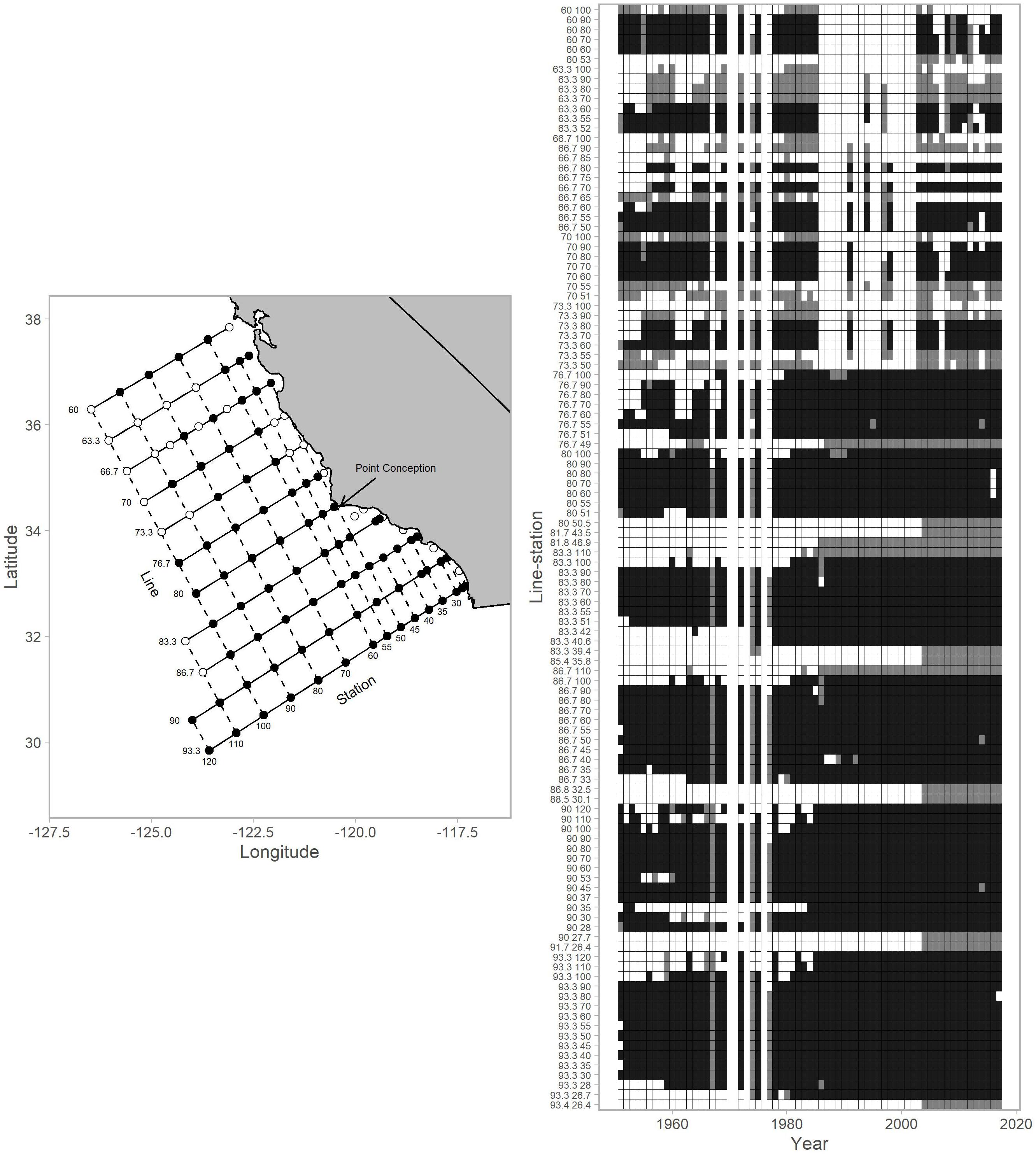
Figure 1. Map of stations within the CalCOFI survey grid and the data availabilities for each individual station (referenced by line-station) for 1951–2017. The map (left column) shows stations used for this analysis (black points) and those that were not (white points). The arrow indicates the location of Point Conception. The data availability plot (right column) shows survey records for years with winter-spring values (black tiles), summer-autumn values (gray tiles; not used in analysis), and no coverage (white tiles). CalCOFI shifted from annual to mostly triennial sampling from 1971–1983 resulting in no surveys in some years. In the early years of CalCOFI, the survey area extended north to British Columbia, Canada and south to Baja California, Mexico (not shown).

CalCOFI samples a myriad of physical factors throughout the water column with a conductivity temperature depth instrument (McClatchie, 2014; Gallo et al., 2019). We focus here on temperature and salinity because these variables are known to impact the distribution and abundance of many marine species (Thompson et al., 2014, 2017). For each station, we calculate mean temperature and salinity between the surface and 100 m and average these means across winter and spring cruises for each station.

The main, long-running CalCOFI biological observations are collected with plankton nets. We focus on ichthyoplankton collected with bongo nets lowered to 210 m (or within 10 m of the bottom at shallow stations) and towed to the surface at a constant speed and at a 45° angle (McClatchie, 2014). Quantifying the abundance of larval fishes is a comprehensive method for assessing the dynamics of most fishes in an ecosystem because although adults occupy different habitats, larval fishes from most species reside in the upper 200 m of the water column and can thus be sampled simultaneously. Several studies demonstrate that ichthyoplankton abundance correlates with the spawning stock biomass of fishes (Moser and Watson, 1990; Moser et al., 2001; Ralston et al., 2003; Ralston and MacFarlane, 2010). CalCOFI plankton samples are preserved at sea in a tris-buffered 5% formalin solution. Ichthyoplankton are identified in a laboratory based on morphology (Moser, 1996). CalCOFI provides time series for hundreds of fishes. Raw larval counts are multiplied by a standard haul factor that accounts for differences in water filtered and divided by the percent of the samples with high zooplankton volumes are often subsampled (Smith, 1977). Final abundances are expressed as larvae per 10 m² surface area. CalCOFI surveys typically sample each of the stations we use in this study 1–4 times per year (Figure 1), and we calculate annual averages from winters and springs. Note that CalCOFI shifted from annual to mostly triennial sampling from 1971 to 1983 resulting in no surveys in some years (e.g., 1979).

Many of the fishes in this study share similar adult habitat affinities and are subject to comparable fishing pressure. Both factors are known to comparably and predictably affect fish population dynamics (Hsieh et al., 2005). To evaluate whether fishes in particular groups exhibit similar patterns of synchrony, we assign each taxa to five groups delineated by Hsieh et al. (2005): oceanic-unfished, coastal-fished, coastal-oceanic-fished, coastal-bycatch, and coastal-unfished. For each species, we select time series with at least 25% non-zero values as some species are only rarely observed at particular stations. For example, some mesopelagic fishes are never or very rarely found at shallow, coastal stations.

Finally, we generate time series of single value Shannon diversity index values (H_s,t) using the equation:

$$H_{s,t}=-\sum _{i=1}^R{p}_{i,s,t}\log \left(p_{i,s,t}\right)(1)$$

at each station (s) in year (t) for species (i). The proportional abundance (p) is multiplied by the natural logarithm of p and summed from species i to the total number of species (R). A single H value was calculated across winter and spring for each year and station. Additionally, the Shannon diversity values were calculated based on all the species reported, which in most cases included additional species to the 36 fish taxa in the single-species analysis. Although we can now identify almost all taxa to species, taxonomic knowledge was less developed at the beginning of CalCOFI. To keep time series used to calculated diversity consistent, we group some species to the 1950s level taxonomic resolution. We use 60 taxa in calculations of Shannon diversity and focus on the 36 most common species for single-species analyses.

Synchrony

We conduct and compare correlational and co-prediction analyses to evaluate synchrony among stations for two physical parameters (temperature and salinity), abundances of 36 fish taxa, and fish diversity. In addition, we evaluate the spatial extent of shared dynamics north and south of Point Conception. Specifically, we quantify the proportion of stations that are significantly synchronous with paired stations within and between northern and southern regions. We follow this analysis by calculating the mean Euclidian distance (km) separating significantly synchronous stations in the north and south. Finally, we assess if synchrony patterns vary among the five fish groups (e.g., ocean-nonfished, coastal-fished). We determine if north-south synchrony patterns differ depending on whether synchrony was assessed with correlation vs. co-prediction analyses.

Correlation

We calculate correlation coefficients (i.e., correlational synchrony) between time series from combinations of station pairs with time lag-0. Our criteria for significance is a statistically significant Spearman’s rho coefficient (p < 0.05). We do not apply sequential Bonferroni corrections that alleviate type-1 error that can arise with multiple testing because our objective is to compare results from correlation and co-prediction analyses rather than evaluate the significance of any one particular time-series.

Co-prediction

A key step in EDM co-prediction analysis is to identify the dimensionality of the data. In nature, a number of physical and environmental factors drive a population; a time series is a one-dimensional observation of the factors’ effects on the population. Fortunately, ecological models do not require analysts to identify all of the factors, rather a comparatively few number of variables can be representative of the dynamics (Schaffer and Kot, 1985). Similarly, Takens’ theorem, a tenet of EDM, formalizes this idea that a single time series and some number of lags (dimension; E) are representative of system dynamics (Takens, 1981; Sugihara and May, 1990). Per Takens’ theorem, an M-dimensional system converges to a d-dimensional attractor, and a single time series of observations y_t,t = 1,2,…,T and lagged coordinates of y (at time step τ) Y_t = {y_t,y_t−τ,…,y_t−Eτ} can reconstruct the d-dimensional attractor (Takens, 1981). This requires that a time series is sufficiently long to capture attractor dynamics.

Simplex projection (hereafter referred to as simplex) along with sequentially locally weighted global linear maps (s-map) are two key EDM forecasting methods. The distinction is that simplex identifies the dimensionality of the system, and s-map characterizes the data as linear or non-linear (Sugihara, 1994). S-map will generally outperform simplex if system dynamics are non-linear.

We first identify the dimensionality of time series in the CalCOFI dataset with simplex. Simplex projection takes a weighted average of the nearest neighbors’ trajectories depending on the specified dimension (E). Given an E, a time series and its E-lagged coordinates, we seek to predict a value ${\widehat{y}}_{t+1}$. In order to predict this value, we use the Euclidean distance d(y_t,y_s) between y_t and y_s and calculate the weights w_i(t) as:

$$w_i\left(t\right)=\exp \left(\frac{-d(y_t,y_{n(t,i)})}{d(y_t,y_{n(t,1)})}\right),(2)$$

where n(t,i) specifies the index of the i-th closest neighbor to y_n(t,1). The prediction ${\widehat{y}}_{t+1}$ is:

$${\widehat{y}}_{t+1}=\frac{\left({\sum }_{i=1}^{E+1}{w}_i(t)y_{n(t,i)+1}\right)}{{\sum }_{i=1}^{E+1}{w}_i\left(t\right)}(3)$$

We use leave-one-out cross-validation and select the E with the highest correlation between predicted and observed values. We evaluate E values ranging from 1 to 10 and identify the best-fitting E for each time series.

Next, we evaluate co-prediction in which we take the best-fitting E for one time series (library) and predict values in another time series (predictee) with simplex. Co-prediction quantifies the dynamic similarity between time series, and has been used to identify interspecific and species-environment dynamics (Liu et al., 2014) and nonlinearities (Liu et al., 2012) in the Northwest Atlantic. We conclude significant co-prediction if there are positive and statistically significant correlations between predicted and observed values (ρ > 0; p < 0.05) and mean absolute scaled error (MASE) values less than 1. Consider a dataset from timesteps t = 1,…,n. We generated a hindcast prediction, F_t, at each timestep. Forecast error was:

$$e_t=Y_t-F_t(4)$$

where Y_t is the observation at time t. Scaled error q_t was:

$$q_t=\frac{e_t}{\frac{1}{n-1}{\sum }_{i=2}^n\left|Y_i-Y_{i-1}\right|}(5)$$

and MASE was:

$$MASE=mean\left(\left|q_t\right|\right)(6)$$

A MASE value less than 1 indicates that the prediction had lower error than that from a naïve predictor, which uses the prior year value as a prediction (Hyndman and Koehler, 2006). Again, we evaluate co-predictability between stations for each set time series (i.e., salinity, temperature, Shannon index of abundance, and single-species ichthyoplankton) for each station, but do not attempt to conduct co-prediction across sets of time series (e.g., we do not predict salinity from temperature).

Further details on EDM are available in the documentation for the R package “rEDM”¹ and Chang et al. (2017).

Hindcasting

We construct composite libraries (i.e., concatenated time series) of the significantly correlated and significantly co-predicted stations identified here.

We generate hindcast predictions from three data scenarios for each time series. Consider time series A from a specific station for a particular data set (e.g., salinity). We s-map hindcast (leave-one-out) values of time series A from: (1) time series A; (2) the composite library of time series A and time series correlated with A; and (3) the composite library of time series A and time series co-predicted by A. Once again, we replicate these three scenarios for each of the time series but do not attempt comparisons between data sets (e.g., predicting Shannon index from salinity). Our goal here is to quantify the ability of correlated and co-predicted stations to improve hindcast skill.

We use s-map with leave-one-out cross validation to evaluate hindcast skill. S-map is an extension of simplex that has an additional parameter (θ) that controls the strength of nearest-neighbor weighting. S-map can make both linear (θ = 0) and non-linear (θ > 0) predictions (Sugihara, 1994). We select E and θ from time series A based on the values that maximize the correlation between the leave-one-out predictions and observations. We then use the E and θ values with s-map to hindcast values for time series A from time series A, correlated composite libraries, and co-predicted composite libraries. The criteria for statistical significance is positive correlations between predicted and observed values (ρ > 0, p < 0.05) and lower error than that of a naïve prior year predictor (MASE < 1).

Results

Synchrony

We found evidence of synchrony between stations within all time series (salinity, temperature, Shannon index, and 36 single-species ichthyoplankton abundances) with both correlational and co-prediction analyses. Generally, there were many more correlational relationships than co-predicted relationships (Figure 2). Each of the 81 stations was correlated and co-predicted with at least one other station for each of the temperature, salinity, and Shannon index data.

FIGURE 2

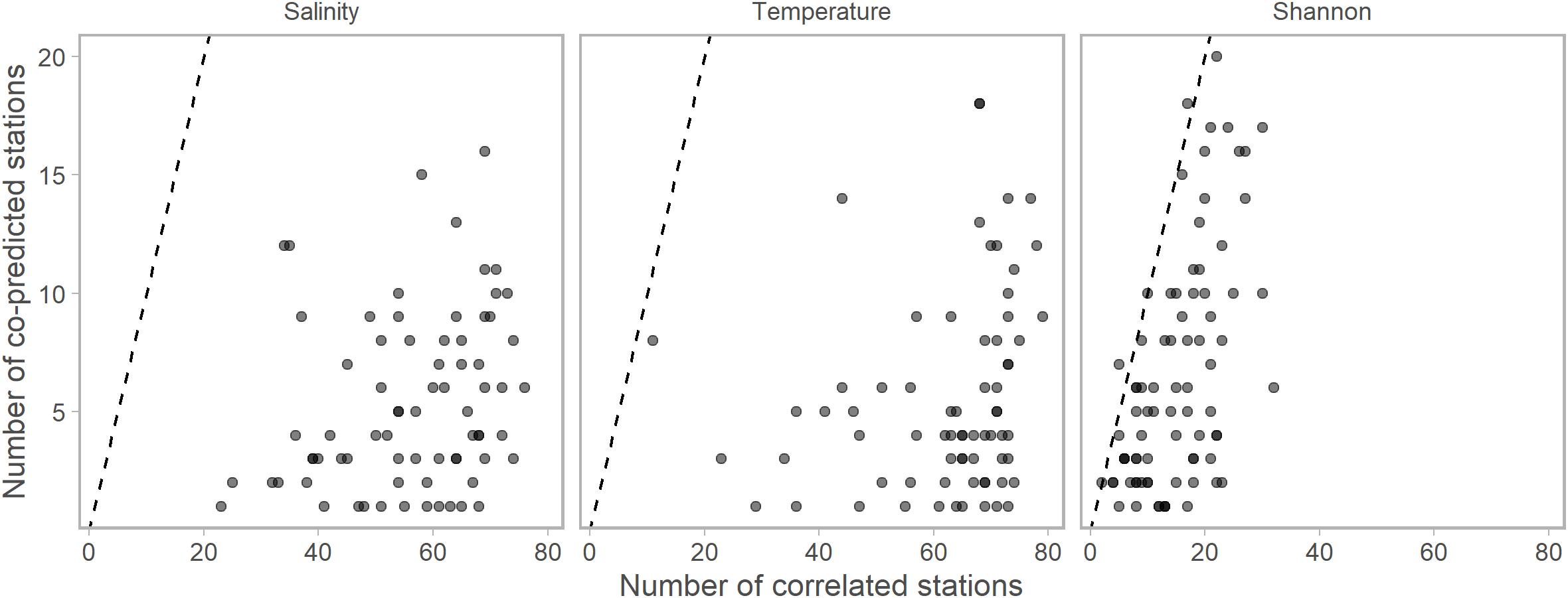
Figure 2. The numbers of significantly correlated vs. numbers of significantly co-predicted stations for salinity, temperature, and Shannon indices of diversity. Each point represents the numbers of each correlated or co-predicted with a particular station (e.g., station A is correlated with 70 stations and co-predicted with 10 stations). Points are slightly transparent to allow overplotting. For nearly all stations, the numbers of correlated stations were higher than the number of co-predicted stations. Dashed lines indicate the one to one line. Composite libraries were composed of correlated or co-predicted stations based on these results.

Correlated and co-predicted stations were most concentrated south of Point Conception. A minority of the correlated pairs are north of Point Conception: 7% for salinity, 8% for temperature, and 17% for Shannon index (Table 1). We found a similar pattern for co-predicted pairs north of Point Conception: 11% for salinity, 18% for temperature, and 6% for Shannon index (Table 1). Note, that 22 of the 81 stations (27%) were located north and 59 of 81 stations (73%) were located south of Point Conception. Generally, stations closer to shore and south had the highest correlation and co-prediction with other stations (Figure 3).

TABLE 1

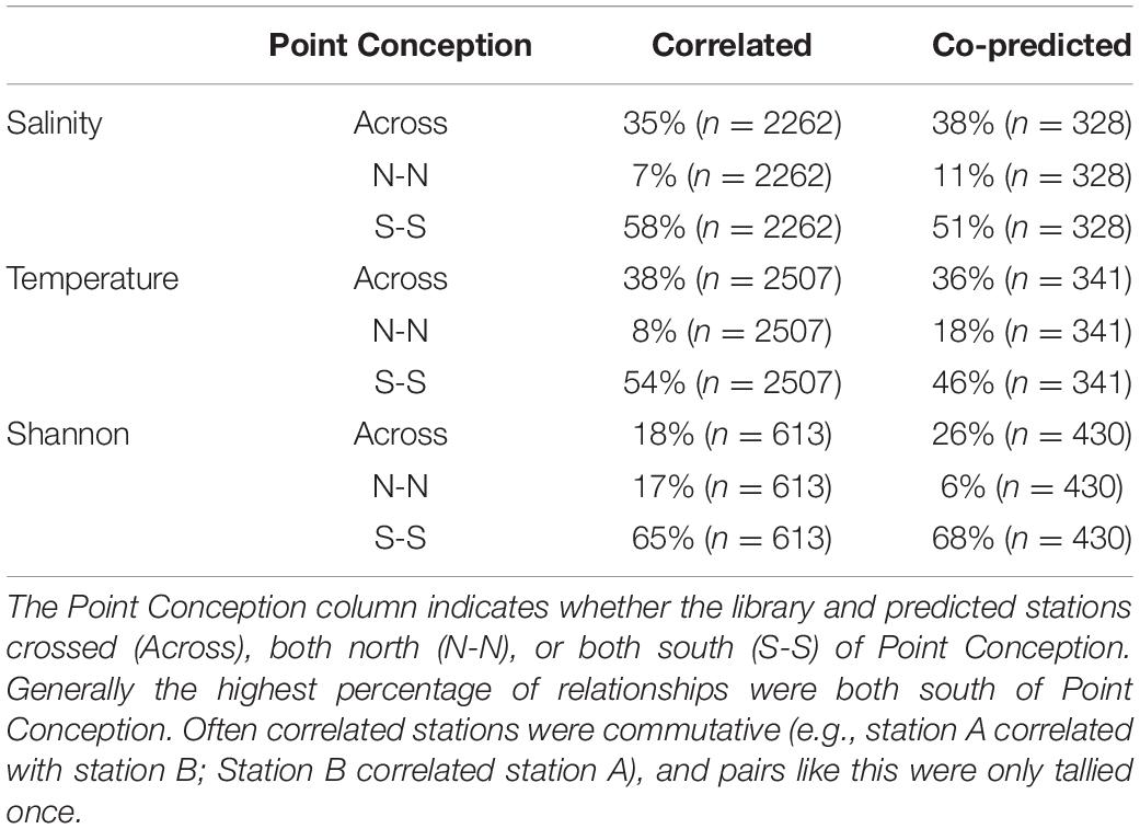
Table 1. Percentages of correlated and co-predicted (number of unique station pairs in parantheses) for salinity, temperature, and Shannon index.

FIGURE 3

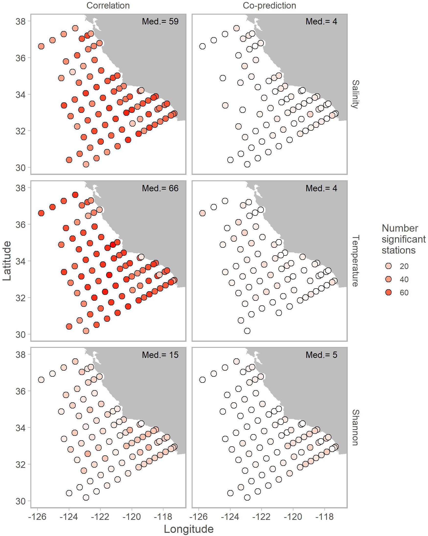
Figure 3. Map of correlated (left column) and co-predicted (right column) stations shown with shades of red. The number of correlated stations was highest for salinity (first row) and temperature (second row). Median number of significant stations are shown in the top right of each panel.

Adjusting for the distribution of stations north (22 stations) and south (59) of Point Conception by representing values in terms of proportions (e.g., 10 out of a possible 22 and 12 of a possible 59) for each library station resulted in slightly more balanced relationships across Point Conception. Stations south of Point Conception co-predicted with roughly the same proportions of stations north and south for salinity, temperature, and Shannon index (Figure 4). Library stations north of Point Conception were more co-predicted with stations north for salinity and temperature, whereas the proportions for Shannon index were roughly equal (Figure 5).

FIGURE 4

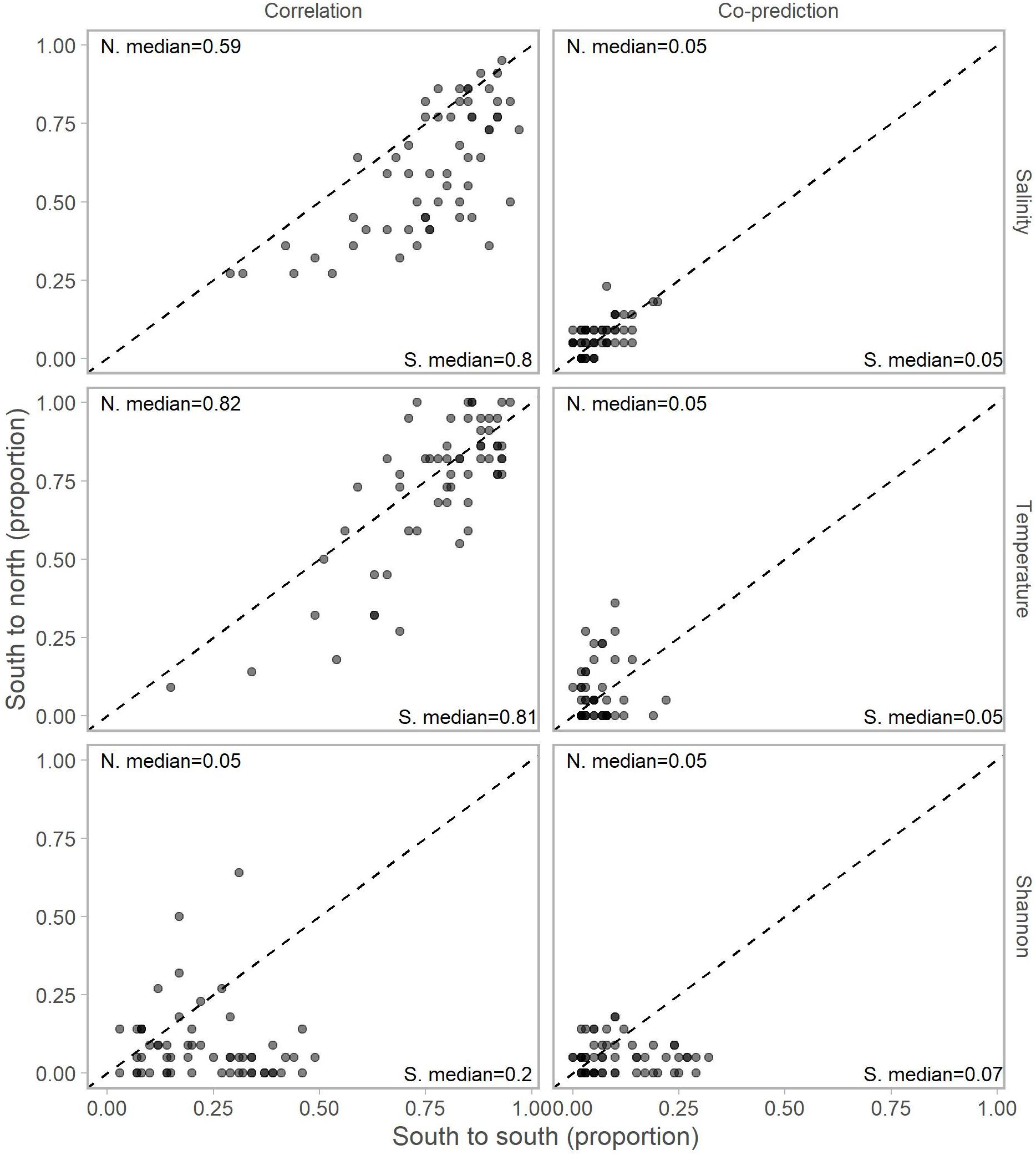
Figure 4. Proportions of south stations correlated (left column) and co-predicted (right column) with stations south (x-axis) and north (y-axis) of Point Conception. There were 59 stations south and 22 stations of Point Conception. Panels show results for the three data types: salinity (top row), temperature (middle row), and Shannon indices (bottom row). The median proportions for predicted stations south (bottom right of each panel) and north (top left of each panel) of Point Conception. The dashed line shows the one-to-one line.

FIGURE 5

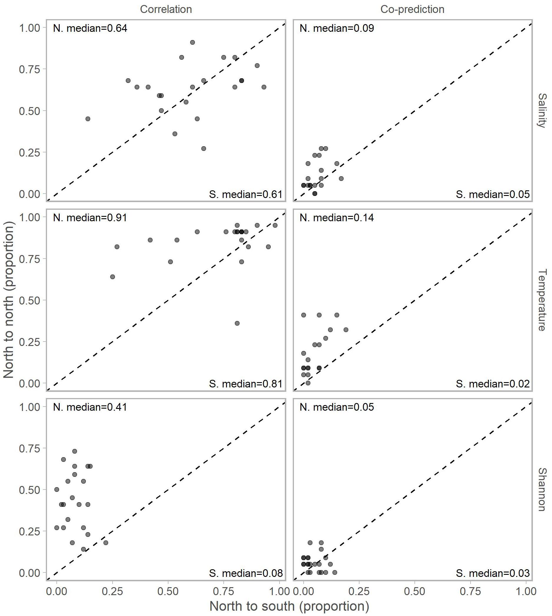
Figure 5. Proportions of north stations correlated (left column) and co-predicted (right column) with stations south (x-axis) and north (y-axis) of Point Conception. There were 59 stations south and 22 stations of Point Conception. Panels show results for the three data types: salinity (top row), temperature (middle row), and Shannon indices (bottom row). The median proportions for predicted stations south (bottom right of each panel) and north (top left of each panel) of Point Conception. The dashed line shows the one-to-one line.

A majority of the predictee stations for single-species ichthyoplankton library stations were concentrated south of Point Conception (Table 2). For library stations north of Point Conception, at least half of the predicted stations were south of Point Conception for coastal-oceanic-fished and oceanic species (Table 2). For library stations south of Point Conception, at least half of the predicted stations were also south for coastal-fished, coastal-oceanic-fished, and oceanic species categories (Table 2).

TABLE 2

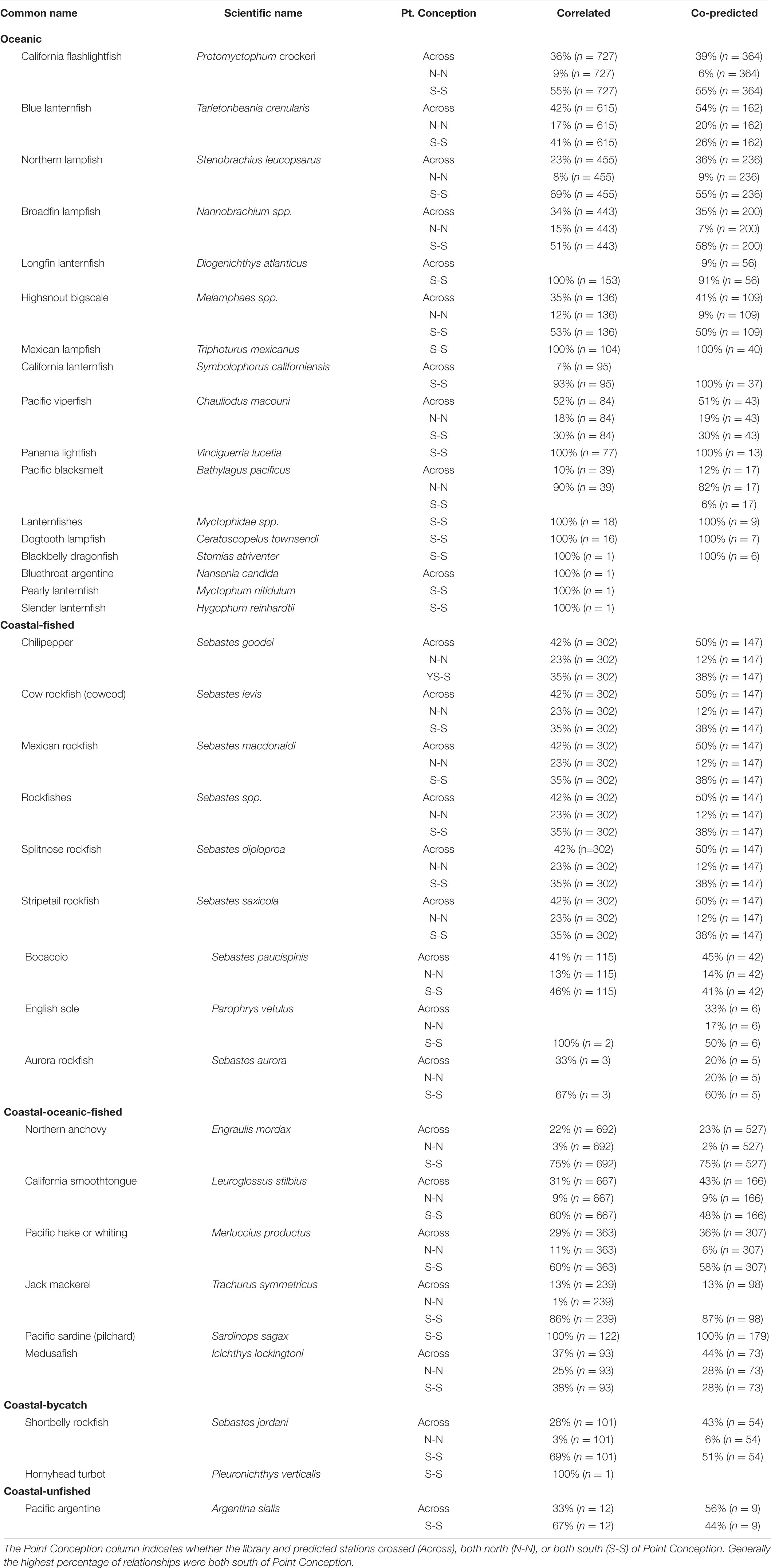
Table 2. Percentages of correlated and co-predicted (number of unique station pairs in parantheses) for individual species grouped by category.

Composite Libraries

Individual stations showed evidence of hindcast skill. Leave-one-out predictions for a particular time series were significant in 27 stations for salinity, 36 for temperature, and 33 for Shannon index of 81 total stations (Table 3).

TABLE 3

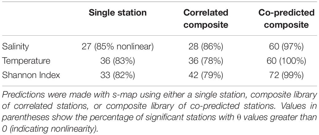
Table 3. Numbers of significantly predicted stations for salinity, temperature, and Shannon indices of diversity.

Composite libraries generally resulted in a greater number of significantly predicted stations. The number of significantly predicted stations from composite libraries of correlated stations was 28 for salinity, 36 for temperature, and 42 for Shannon index (Table 3). Predictions from composite libraries of co-predicted stations were significant in 60 stations for salinity, 60 for temperature, and 72 stations for Shannon index (Table 3). For salinity and Shannon index, co-prediction was a more robust method of identifying shared dynamics than correlation.

Generally, significant hindcast skill was highest with nonlinear predictions, indicated by θ values greater than 0. Nonlinear predictions resulted in significance for roughly 80% of the stations in the single station and composite library scenarios (Table 3). For the co-predicted composite library scenario, nonlinear s-map predictions accounted for nearly all the significant results (Table 3).

The CalCOFI survey has variable temporal and spatial sampling frequencies due to logistical and financial challenges common to any long-term ecological survey. Stations off northern California in the CalCOFI grid had stretches with no winter and spring surveys. Because we compare s-map predictions to lagged observations, assuming a lagged observation from say 10 years prior may bias MASE calculations. In other words, a poor predictor compared to a lagged observation from many years prior may result in lower MASE values. To control for this, we filtered time series such that the maximum gap was 3 years or less and recalculated MASE. The number of significant stations was relatively unchanged, and the number of significantly co-predicted composite library stations decreased by 1–3 stations (Supplementary Table 1).

Inclusion of co-predicted stations improved hindcast skill of Shannon index for mostly offshore stations (Figure 6). Additionally, composite libraries resulted in significant predictability for all three of salinity, temperature, and Shannon index in 38 of 81 stations. Although there were some cases, particularly for salinity and Shannon index, where predictions from composite libraries of co-predicted stations had MASE values of 0.6 (indicating that error from predictions was 60% the error from a lagged observation; Figure 6).

FIGURE 6

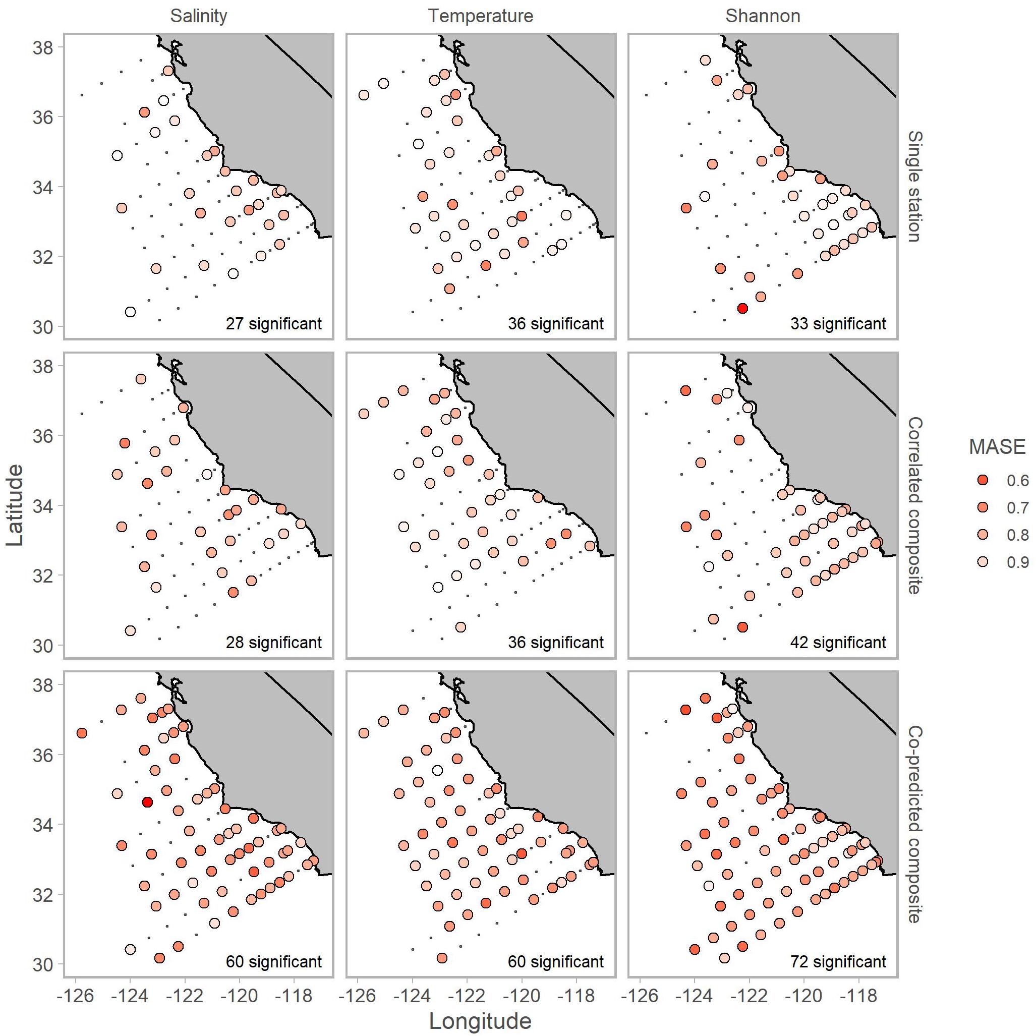
Figure 6. Locations of stations with significant hindcast s-map predictive skill for salinity (left column), temperature (middle column) and Shannon index (right column). Predictions used single station (top row), correlated composite libraries (middle row) and co-predicted composite libraries (bottom row). Shading indicates MASE values. A MASE of 0.6, for example, indicates that the error from s-map predictions is on average 60% of the error from a na ve predictor (i.e., lagged observation). The number of significant stations is shown in the bottom right of each panel.

Prediction for individual species was highest with co-predicted composite libraries. For many species, hindcast skill was highest with composite libraries of co-predicted stations, and this trend was strongest in oceanic and coastal-fished species (Table 4).

TABLE 4

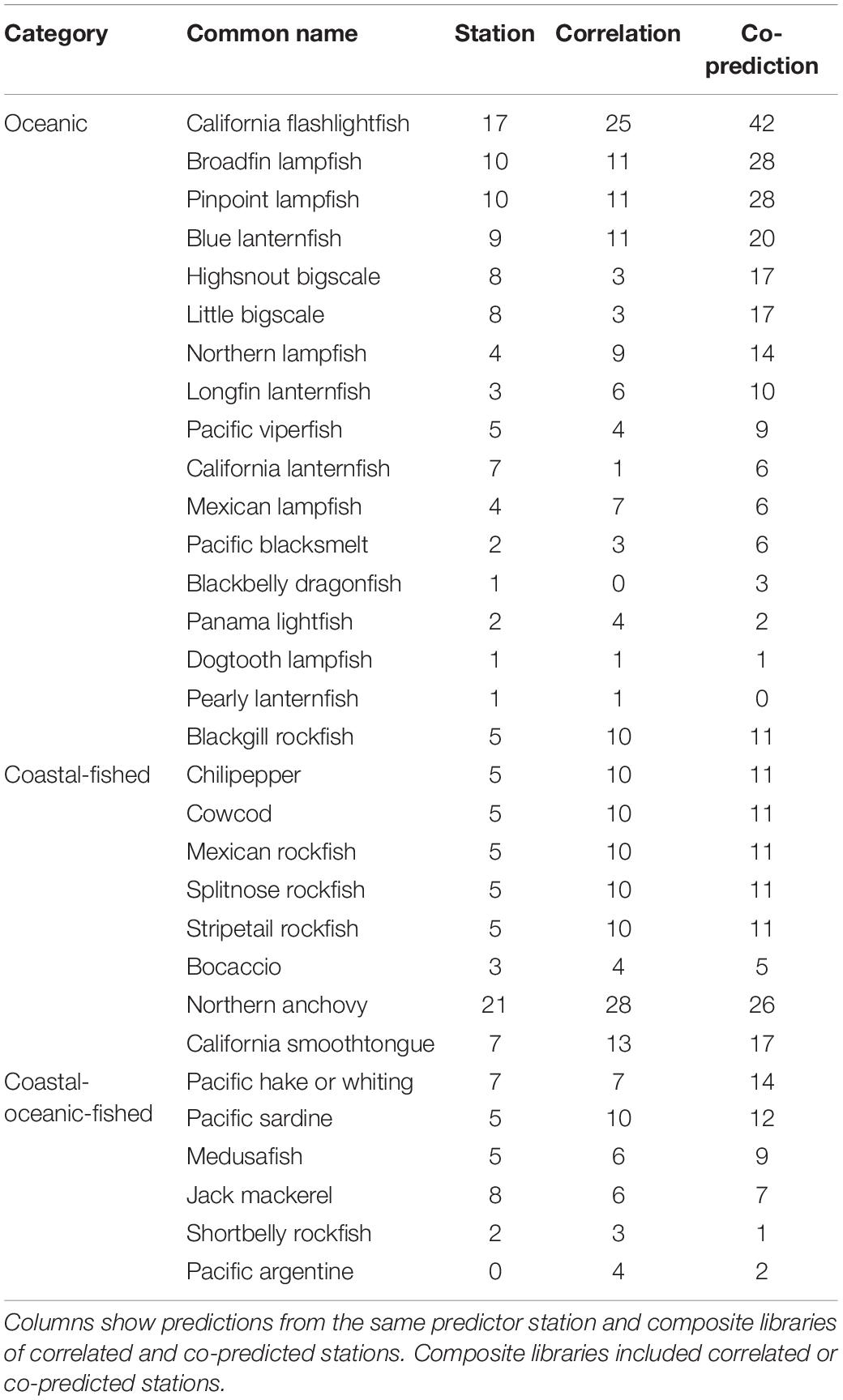
Table 4. Numbers of significantly predicted stations with s-map prediction for each species, arranged by category.

Discussion

We find evidence of spatially shared dynamics in salinity, temperature, Shannon index, and individual ichthyoplankton species as measured by correlation and co-prediction. Leveraging knowledge of shared dynamics via composite libraries of correlated or co-predicted stations generally improved hindcast skill across all data types. However, although synchrony is more evident from correlation than co-prediction, co-prediction is a more robust method to significantly hindcast salinity, temperature, Shannon index, and nearly all single-species ichthyoplankton. Taken together, we demonstrate the utility of co-prediction in identifying shared dynamics and find evidence of widespread nonlinear spatial structure in physical and biological observations across the CalCOFI survey area. To our knowledge, this study serves as the first evaluation of station-specific hindcast skill of the CalCOFI data set.

Identifying shared dynamics with co-prediction is an important step in constructing composite libraries. Previous studies that implemented composite libraries used all available time series from individual species (Hsieh et al., 2008) or locations (Glaser et al., 2014; Clark et al., 2015). Our results show that identifying shared dynamics with co-prediction is an important step to improve hindcast skill. Longer composite libraries composed of more stations (identified through correlation) did not result in higher hindcast skill than co-predicted stations, with the exception of Shannon index. While we did not explicitly have a scenario of composite libraries with all 81 stations, composite libraries for salinity and temperature mostly included between 70 and 80 correlated stations. Co-prediction quantifies the degree to which two time series are generated from the same underlying process and has the potential to identify relationships in the absence of positive correlation (Engle and Granger, 1987).

We found evidence of nonlinear relationships in the CalCOFI survey data. A majority of the significant results came from nonlinear predictions, with s-map θ values greater than 0, across data types and composite library scenarios. These findings are consistent with previous analyses of CalCOFI data which found nonlinearities in biological time series (Hsieh et al., 2005). These studies utilized out-of-sample forecasting, in contrast to the methods used here, but found that physical time series had high dimensionality and linear dynamics. Thus, it is likely that fish populations have nonlinear responses to environmental forces and have nonlinear relationships across space.

While this study focuses on hindcasting, the methods used here may be extended to out-of-sample forecasting to better identify and predict regime shifts. The transition to out-of-sample forecasting may yield insight to the characteristics of a system undergoing a regime shift. For example, a system undergoing a regime shift may be characterized by a composite library of co-predicted stations undergoing a decrease in forecast skill. Additional indicators may be a shift in the number and orientation of co-predicted stations or a transition between linear and nonlinear dynamics. If analyses extend to include multivariate analyses, there may be time-varying changes in interactions, similar to those identified in Deyle et al. (2016).

The California Current is characterized by physical and biological regimes, and here we show that stations across space demonstrate shared dynamics through multiple regimes over the roughly 70 year span of CalCOFI observations. Studies of principal components in over 100 time series, both physical and biological, found regime shifts in 1976 and 1989 (Ebbesmeyer et al., 1991; Hare and Mantua, 2000). Shifts in the Pacific Decadal Oscillation from a negative to positive phase were hypothesized to precede shifts in biological regimes (McFarlane and Beamish, 2001; Moser et al., 2001). Indeed, a previous study has identified five ichthyoplankton assemblage regimes in analysis of the southern portion of the CalCOFI survey area (Peabody et al., 2018). The combination of co-prediction, composite libraries, and s-map can potentially improve the capability to track system dynamics of a regime change. This work remains to be done but is a logical next step.

We found shared dynamics to be largely concentrated south of Point Conception, although this result may be influenced by skewed station distributions north and south of Point Conception. Point Conception is a well-known biogeographic break within the CCE (Allen et al., 2006) with sharply contrasting water masses north and south of Point Conception (Lynn et al., 2003). Ocean conditions north of Point Conception tend to be dominated by the equatorward-flowing California Current which is cold and relatively fresh as well as cold, salty upwelled water closer to shore that is induced by strong equatorward winds (Checkley and Barth, 2009). As a result, water temperature often increases abruptly south of Point Conception within the Southern California Bight (Checkley and Barth, 2009; Thompson et al., 2016). Co-prediction identifies shared dynamics between two time series but does not measure causal relationships. Convergent cross mapping (Sugihara et al., 2012) can identify causality between time series, and analyses that apply this method may identify mechanistic relationships between stations. Inclusion of additional oceanographic measurements such as oxygen, phosphate, and silicate may further enhance analyses of the movement and forcing of distinct water masses.

Shannon index have significant hindcast skill in 89% of stations (n = 81). While our focus is on the 60 most-caught taxa (used to calculate Shannon index), our results indicate that there are likely common factors driving shared dynamics across space. Physical conditions cascade to affect zooplankton abundances, which fluctuated in synchrony from 1949 to 1969 (Bernal and McGowan, 1981). Additionally, taxa with similar life histories and adult habitats track each other even when they are uncorrelated with environmental conditions (Hsieh et al., 2005). This is another area of future research, and convergent cross mapping, another EDM method, is one extension to identify causal relationships between populations and environmental conditions or interspecific interactions.

There are multiple possible ecological explanations for the predictability in species like Northern anchovy and bigscales. Recruitment may be an important factor influencing shared ichthyoplankton dynamics in the CalCOFI data. Recruitment generally stabilizes metacommunities (Gouhier et al., 2010, 2011) although the relative levels of recruitment can influence synchrony and stability differently (Townsend and Gouhier, 2019). Additionally, local recruitment synchronizes mussel populations across 1,800 km of coast (Gouhier et al., 2010). The rich time series of available data in the Southern California Bight would allow for analyses relating egg time series (collected on CalCOFI cruises) to ichthyoplankton time series to young-of-year surveys and adult catches to evaluate interactions across all life history stages. EDM works best at predicting recruitment for short-lived, fast-growing species (Munch et al., 2018), and the inclusion of multiple variables may further improve forecast skill. Oceanographic currents in the Southern California Bight have been characterized to identify metapopulation networks (Watson et al., 2011).

While the EDM approach is generally robust to some missing values, additional modeling approaches may not be. The composite library approach has higher predictive skill than using the previous year’s value as the forecast. In an analysis of multiple time series forecast methods, this naïve predictor had the highest short-term predictive skill for 2,379 time series of vertebrate population indices (Ward et al., 2014). Shannon index results were likely more predictable as they integrate the year-to-year variability in individual species. Species like bigscales, blue lanternfish, rockfish, Northern anchovy, and Pacific hake all had the most predictable dynamics suggesting that there may be a small number of species driving Shannon index in each year.

Evaluation of out-of-sample predictability was beyond the scope of this study but is a logical next step. Out-of-sample forecasting skill will likely increase if causal relationships exist in the CalCOFI data. Convergent cross mapping (Sugihara et al., 2012) and its spatial applications (Clark et al., 2015) are natural extensions of this analysis and may identify relationships between physical variables like temperature and salinity and biological variables like Shannon index of diversity. The CalCOFI dataset is an ideal dataset for such analysis due to the high spatiotemporal resolution and multiple types of observations. Comparing temperature and salinity directly to ichthyoplankton time series misses key components of the community structure. Likely, there are multiple levels of interactions relating physical conditions to phytoplankton to zooplankton to ichthyoplankton (Thompson et al., 2018). Additionally, analysis may need to adopt a finer temporal scale to identify seasonal drivers. Here, we used averages of physical and biological measurements across winter and spring, which may have smoothed signal in the data. S-map coefficients may elucidate time-varying interactions between biological and physical data sets (Deyle et al., 2016; Ushio et al., 2018). Finally, additional methodologies such as EDM Gaussian processes (Munch et al., 2017; Rogers and Munch, 2020) and regularized s-map (Cenci et al., 2019) may offer improvements in both in-sample and out-of-sample prediction skill.

The analysis we have presented here, and the analytic next steps outlined above, are motivated by both the desire to understand the ecological dynamics of the CCE and the need to identify analytic methods that can support future survey design/reorganization efforts. There are numerous financial and logistical challenges associated with conducting large-scale surveys, and it is difficult to maintain constant sampling efforts year to year. Co-prediction and composite libraries can provide a means of prioritizing survey sites by identifying partial redundancies in the CalCOFI survey grid. In the case that sampling efforts reduce, locations with strongly shared dynamics may be redundant, in that sampling in these areas may not provide additional information. Locations without shared dynamics may be high priorities because they contribute to a more comprehensive survey of an area.

Data Availability Statement

Publicly available datasets were analyzed in this study. This data can be found here: https://calcofi.org/ccdata.html.

Author Contributions

PTK, GS, ART, and BXS designed the study. PTK conducted that analysis and wrote the manuscript. GS, ART, and BXS contributed and edited the text. All authors contributed to the article and approved the submitted version.

Funding

PTK and BXS received funding from the NOAA Quantitative Ecology and Socioeconomics Training program. GS was supported by DoD-Strategic Environmental Research and Development Program 15 RC-2509, NSF DEB-1655203, NSF ABI-1667584, DOI USDI-NPS P20AC00527, the McQuown Fund and the McQuown Chair in Natural Sciencies, University of California, San Diego.

Conflict of Interest

The authors declare that the research was conducted in the absence of any commercial or financial relationships that could be construed as a potential conflict of interest.

Acknowledgments

We express our deep gratitude to the crews of the CalCOFI research vessels for helping collect the samples, including, but not limited to, David Ambrose, Noelle Bowlin, Sherri Charter, Dave Griffith, Amy Hays, Bryan Overcash, and Sue Manion. Hao Ye, Ethan Deyle, and Chase James provided valuable technical advice regarding EDM analyses. Thanks to the reviewers for providing comments that improved the quality of the manuscript.

Supplementary Material

The Supplementary Material for this article can be found online at: https://www.frontiersin.org/articles/10.3389/fmars.2020.557940/full#supplementary-material

Footnotes

1. ^ https://github.com/ha0ye/rEDM

References

Allen, L. G., Pondella, D. J., and Horn, M. H. (2006). Ecology of Marine Fishes: California and Adjacent Waters. Berkeley, CA: University of California Press.

Google Scholar

Bellamy, P., Rothery, P., and Hinsley, S. (2003). Synchrony of woodland bird populations: the effect of landscape structure. Ecography 26, 338–348. doi: 10.1034/j.1600-0587.2003.03457.x

PubMed Abstract | CrossRef Full Text | Google Scholar

Bernal, P. A., and McGowan, J. A. (1981). Advection and Upwelling in the California Current. In: Coastal Upwelling. Washington, DC: American Geophysical Union, 381–399.

Google Scholar

Bjørnstad, O. N., Ims, R. A., and Lambin, X. (1999). Spatial population dynamics: analyzing patterns and processes of population synchrony. Trends Ecol. Evol. 14, 427–432. doi: 10.1016/s0169-5347(99)01677-8

CrossRef Full Text | Google Scholar

Bograd, S. J., Buil, M. P., Di Lorenzo, E., Castro, C. G., Schroeder, I. D., Goericke, R., et al. (2015). Changes in source waters to the Southern California bight. Deep Sea Res. Part II Top. Stud. Oceanogr. 112, 42–52. doi: 10.1016/j.dsr2.2014.04.009

CrossRef Full Text | Google Scholar

Buonaccorsi, J. P., Elkinton, J. S., Evans, S. R., and Liebhold, A. M. (2001). Measuring and testing for spatial synchrony. Ecology 82, 1668–1679. doi: 10.1890/0012-9658(2001)082%5B1668:matfss%5D2.0.co;2

CrossRef Full Text | Google Scholar

Cenci, S., Sugihara, G., and Saavedra, S. (2019). Regularized S−map for inference and forecasting with noisy ecological time series. Methods Ecol. Evol. 10, 650–660. doi: 10.1111/2041-210x.13150

CrossRef Full Text | Google Scholar

Chang, C.-W., Ushio, M., and Hsieh, C-h. (2017). Empirical dynamic modeling for beginners. Ecol. Res. 32, 785–796. doi: 10.1007/s11284-017-1469-9

CrossRef Full Text | Google Scholar

Checkley, D. M. Jr., and Barth, J. A. (2009). Patterns and processes in the California current system. Prog. Oceanogr. 83, 49–64. doi: 10.1016/j.pocean.2009.07.028

CrossRef Full Text | Google Scholar

Clark, A. T., Ye, H., Isbell, F., Deyle, E. R., Cowles, J., Tilman, G. D., et al. (2015). Spatial convergent cross mapping to detect causal relationships from short time series. Ecology 96, 1174–1181. doi: 10.1890/14-1479.1

CrossRef Full Text | Google Scholar

Cressie, N., and Wikle, C. K. (2015). Statistics for Spatio-temporal Data. Hoboken, NJ: John Wiley & Sons.

Google Scholar

Deyle, E. R., Fogarty, M., Hsieh C-h, Kaufman, L., MacCall, A. D., Munch, S. B., et al. (2013). Predicting climate effects on Pacific sardine. Proc. Natl. Acad. Sci. U.S.A. 110, 6430–6435. doi: 10.1073/pnas.1215506110

PubMed Abstract | CrossRef Full Text | Google Scholar

Deyle, E. R., May, R. M., Munch, S. B., and Sugihara, G. (2016). Tracking and forecasting ecosystem interactions in real time. Proc. R. Soc. B Biol. Sci. 283:20152258. doi: 10.1098/rspb.2015.2258

PubMed Abstract | CrossRef Full Text | Google Scholar

Ebbesmeyer, C. C., Cayan, D. R., McLain, D. R., Nichols, F. H., Peterson, D. H., and Redmond, K. T. (1991). “1976 step in the Pacific climate: forty environmental changes between 1968-1975 and 1977-1984,” in Proceedings of the Seventh Annual Pacific Climate (PACLIM) Workshop, Pacific Grove, CA.

Google Scholar

Engle, R. F., and Granger, C. W. (1987). Co-integration and error correction: representation, estimation, and testing. Econometrica 55, 251–276. doi: 10.2307/1913236

CrossRef Full Text | Google Scholar

Fromentin, J.-M., Gjøsæter, J., Bjørnstad, O. N., and Stenseth, N. C. (2000). Biological processes and environmental factors regulating the dynamics of the Norwegian Skagerrak cod populations since 1919. ICES J. Mar. Sci. 57, 330–338. doi: 10.1006/jmsc.1999.0638

CrossRef Full Text | Google Scholar

Gallo, N. D., Drenkard, E., Thompson, A. R., Weber, Wilson-Vandenberg, D., McClatchie, S., et al. (2019). Bridging from monitoring to solutions-based thinking: lessons from CalCOFI for understanding and adapting to marine climate change impacts. Front. Mar. Sci. 6:695.

Google Scholar

Glaser, S. M., Ye, H., and Sugihara, G. (2014). A nonlinear, low data requirement model for producing spatially explicit fishery forecasts. Fish. Oceanogr. 23, 45–53. doi: 10.1111/fog.12042

CrossRef Full Text | Google Scholar

Gouhier, T. C., and Guichard, F. (2014). Synchrony: quantifying variability in space and time. Methods Ecol. Evol. 5, 524–533. doi: 10.1111/2041-210x.12188

CrossRef Full Text | Google Scholar

Gouhier, T. C., Guichard, F., and Menge, B. A. (2010). Ecological processes can synchronize marine population dynamics over continental scales. Proc. Natl. Acad. Sci. U.S.A. 107, 8281–8286. doi: 10.1073/pnas.0914588107

PubMed Abstract | CrossRef Full Text | Google Scholar

Gouhier, T. C., Menge, B. A., and Hacker, S. D. (2011). Recruitment facilitation can promote coexistence and buffer population growth in metacommunities. Ecol. Lett. 14, 1201–1210. doi: 10.1111/j.1461-0248.2011.01690.x

PubMed Abstract | CrossRef Full Text | Google Scholar

Hare, S. R., and Mantua, N. J. (2000). Empirical evidence for North Pacific regime shifts in 1977 and 1989. Prog. Oceanogr. 47, 103–145. doi: 10.1016/s0079-6611(00)00033-1

CrossRef Full Text | Google Scholar

Harvey, C. J., Garfield, N., Williams, G. D., Tolimieri, N., Schroeder, I., Andrews, K. S., et al. (2019). “Ecosystem status report of the california current for 2019: a summary of ecosystem indicators compiled by the california current integrated ecosystem assessment team (CCIEA),” in US Department of Commerce, NOAA Technical Memorandum. NMFS-NWFSC-149.

Google Scholar

Hewitt, R. P. (1988). Historical review of the oceanographic approach to fishery research. Calif. Coop. Oceanic Fish. Invest. Rep. 29, 27–41.

Google Scholar

Holyoak, M., and Lawler, S. P. (1996). Persistence of an extinction−prone predator−prey interaction through metapopulation dynamics. Ecology 77, 1867–1879. doi: 10.2307/2265790

CrossRef Full Text | Google Scholar

Hsieh, C-H., Anderson, C., and Sugihara, G. (2008). Extending nonlinear analysis to short ecological time series. Am. Naturalist 171, 71–80. doi: 10.1086/524202

PubMed Abstract | CrossRef Full Text | Google Scholar

Hsieh, C-H., Reiss, C., Watson, W., Allen, M. J., Hunter, J. R., Lea, R. N., et al. (2005). A comparison of long-term trends and variability in populations of larvae of exploited and unexploited fishes in the Southern California region: a community approach. Prog. Oceanogr. 67, 160–185. doi: 10.1016/j.pocean.2005.05.002

CrossRef Full Text | Google Scholar

Hubbs, C. L. (1948). Changes in the fish fauna of western North America correlated with changes in ocean temperature. J. Mar. Res. 7, 459–482.

Google Scholar

Hyndman, R. J., and Koehler, A. B. (2006). Another look at measures of forecast accuracy. Int. J. Forecasting 22, 679–688. doi: 10.1016/j.ijforecast.2006.03.001

CrossRef Full Text | Google Scholar

Jacox, M. G., Alexander, M. A., Siedlecki, S., Chen, K., Kwon, Y.-O., Brodie, S., et al. (2020). Seasonal-to-interannual prediction of North American coastal marine ecosystems: forecast methods, mechanisms of predictability, and priority developments. Prog. Oceanogr. 183:102307. doi: 10.1016/j.pocean.2020.102307

CrossRef Full Text | Google Scholar

Koenig, W. D. (1999). Spatial autocorrelation of ecological phenomena. Trends Ecol. Evol. 14, 22–26. doi: 10.1016/s0169-5347(98)01533-x

CrossRef Full Text | Google Scholar

Liebhold, A., Koenig, W. D., and Bjørnstad, O. N. (2004). Spatial synchrony in population dynamics. Annu. Rev. Ecol. Evol. Syst. 35, 467–490.

Google Scholar

Liu, H., Fogarty, M. J., Glaser, S. M., Altman, I., Hsieh C-h, Kaufman, L., et al. (2012). Nonlinear dynamic features and co-predictability of the Georges Bank fish community. Mar. Ecol. Prog. Ser. 464, 195–207. doi: 10.3354/meps09868

CrossRef Full Text | Google Scholar

Liu, H., Fogarty, M. J., Hare, J. A., Hsieh C-h, Glaser, S. M., Ye, H., et al. (2014). Modeling dynamic interactions and coherence between marine zooplankton and fishes linked to environmental variability. J. Mar. Syst. 131, 120–129. doi: 10.1016/j.jmarsys.2013.12.003

CrossRef Full Text | Google Scholar

Lynn, R. J., Bograd, S. J., Chereskin, T. K., and Huyer, A. (2003). Seasonal renewal of the California current: the spring transition off California. J. Geophys. Res. Oceans 108:C8.

Google Scholar

McClatchie, S. (2014). “Oceanography of the Southern California current system relevant to fisheries,” in Regional Fisheries Oceanography of the California Current System, (Dordrecht: Springer), 13–60. doi: 10.1007/978-94-007-7223-6_2

CrossRef Full Text | Google Scholar

McClatchie, S., Gao, J., Drenkard, E. J., Thompson, A. R., Watson, W., Ciannelli, L., et al. (2018). Interannual and secular variability of larvae of mesopelagic and forage fishes in the Southern California current system. J. Geophys. Res. Oceans 123, 6277–6295. doi: 10.1029/2018jc014011

CrossRef Full Text | Google Scholar

McFarlane, G. A., and Beamish, R. J. (2001). The re-occurrence of sardines off British Columbia characterises the dynamic nature of regimes. Prog. Oceanogr. 49, 151–165. doi: 10.1016/s0079-6611(01)00020-9

CrossRef Full Text | Google Scholar

Moser, H. G. (1996). The Early Stages of Fishes in the California Current Region: California Cooperative Oceanic Fisheries Investigations: Atlas No 33. Chicago, IL: University of Chicago.

Google Scholar

Moser, H. G., Charter, R. L., Watson, W., Ambrose, D., Hill, K., Smith, P., et al. (2001). The CalCOFI ichthyoplankton time series: potential contributions to the management of rocky-shore fishes. Calif. Coop. Oceanic Fish. Invest. Report 42, 112–128.

Google Scholar

Moser, H. G., and Watson, W. (1990). Distribution and abundance of early life history stages of the California halibut, Paralichthys californicus, and comparison with the fantail sole, Xystreurys liolepis. Calif. Dep. Fish. Game Fish. Bull. 174, 31–84.

Google Scholar

Munch, S. B., Giron-Nava, A., and Sugihara, G. (2018). Nonlinear dynamics and noise in fisheries recruitment: a global meta-analysis. Fish Fish. 19, 964–973. doi: 10.1111/faf.12304

CrossRef Full Text | Google Scholar

Munch, S. B., Poynor, V., and Arriaza, J. L. (2017). Circumventing structural uncertainty: a bayesian perspective on nonlinear forecasting for ecology. Ecol. Complexity 32, 134–143. doi: 10.1016/j.ecocom.2016.08.006

CrossRef Full Text | Google Scholar

Myers, R., Mertz, G., and Bridson, J. (1997). Spatial scales of interannual recruitment variations of marine, anadromous, and freshwater fish. Can. J. Fish. Aqua. Sci. 54, 1400–1407. doi: 10.1139/f97-045

CrossRef Full Text | Google Scholar

Myers, R. A., Mertz, G., and Barrowman, N. (1995). Spatial scales of variability in cod recruitment in the North Atlantic. Can. J. Fish. Aquatic Sci. 52, 1849–1862. doi: 10.1139/f95-778

CrossRef Full Text | Google Scholar

Peabody, C. E., Thompson, A. R., Sax, D. F., Morse, R. E., and Perretti, C. T. (2018). Decadal regime shifts in southern California’s ichthyoplankton assemblage. Mar. Ecol. Prog. Series 607, 71–83. doi: 10.3354/meps12787

CrossRef Full Text | Google Scholar

Perretti, C. T., Munch, S. B., and Sugihara, G. (2013a). Model-free forecasting outperforms the correct mechanistic model for simulated and experimental data. Proc. Natl. Acad. Sci. U.S.A. 110, 5253–5257. doi: 10.1073/pnas.1216076110

PubMed Abstract | CrossRef Full Text | Google Scholar

Perretti, C. T., Sugihara, G., and Munch, S. B. (2013b). Nonparametric forecasting outperforms parametric methods for a simulated multispecies system. Ecology 94, 794–800. doi: 10.1890/12-0904.1

CrossRef Full Text | Google Scholar

Pikitch, E. K., Santora, C., Babcock, E. A., Bakun, A., Bonfil, R., Conover, D. O., et al. (2004). Ecosystem-based fishery management. Science 405, 346–347. doi: 10.1126/science.1098222

PubMed Abstract | CrossRef Full Text | Google Scholar

Pinsky, M. L., Worm, B., Fogarty, M. J., Sarmiento, J. L., and Levin, S. A. (2013). Marine taxa track local climate velocities. Science 341, 1239–1242. doi: 10.1126/science.1239352

PubMed Abstract | CrossRef Full Text | Google Scholar

Ralston, S., Bence, J. R., Eldridge, M. B., and Lenarz, W. H. (2003). An approach to estimating rockfish biomass based on larval production, with application to Sebastes jordani. Fish. Bull. 101, 129–146.

Google Scholar

Ralston, S., and MacFarlane, B. R. (2010). Population estimation of bocaccio (Sebastes paucispinis) based on larval production. Can. J. Fish. Aqua. Sci. 67, 1005–1020. doi: 10.1139/f10-039

CrossRef Full Text | Google Scholar

Ranta, E., Kaitala, V., Lindström, J., and Linden, H. (1995). Synchrony in population dynamics. Proc. R. Soc. Lond. Ser. B Biol. Sci. 262, 113–118.

Google Scholar

Rogers, T. L., and Munch, S. B. (2020). Hidden similarities in the dynamics of a weakly synchronous marine metapopulation. Proc. Natl. Acad. Sci. U.S.A. 117, 479–485. doi: 10.1073/pnas.1910964117

PubMed Abstract | CrossRef Full Text | Google Scholar

Rykaczewski, R. R., and Checkley, D. M. (2008). Influence of ocean winds on the pelagic ecosystem in upwelling regions. Proc. Natl. Acad. Sci. U.S.A. 105, 1965–1970. doi: 10.1073/pnas.0711777105

PubMed Abstract | CrossRef Full Text | Google Scholar

Schaffer, W. M., and Kot, M. (1985). Do strange attractors govern ecological systems? BioScience 35, 342–350. doi: 10.2307/1309902

CrossRef Full Text | Google Scholar

Smith, P. E. (1977). Standard techniques for pelagic fish egg and larva surveys. FAO Fish. Tech. Pap. 175, 1–100.

Google Scholar

Sugihara, G. (1994). Nonlinear forecasting for the classification of natural time series. Philos. Trans. R. Soc. Lond. Ser. A Phys. Eng. Sci. 348, 477–495. doi: 10.1098/rsta.1994.0106

CrossRef Full Text | Google Scholar

Sugihara, G., Beddington, J., Hsieh, C-H, Deyle, E., Fogarty, M., Glaser, S. M., et al. (2011). Are exploited fish populations stable? Proc. Natl. Acad. Sci. U.S.A. 108, E1224–E1225.

Google Scholar

Sugihara, G., May, R., Ye, H., Hsieh, C-H, Deyle, E., Fogarty, M., et al. (2012). Detecting causality in complex ecosystems. Science 338, 496–500. doi: 10.1126/science.1227079

PubMed Abstract | CrossRef Full Text | Google Scholar

Sugihara, G., and May, R. M. (1990). Nonlinear forecasting as a way of distinguishing chaos from measurement error in time series. Nature 344, 734–741. doi: 10.1038/344734a0

PubMed Abstract | CrossRef Full Text | Google Scholar

Sutcliffe, O. L., Thomas, C. D., and Moss, D. (1996). Spatial synchrony and asynchrony in butterfly population dynamics. J. Anim. Ecol. 65, 85–95. doi: 10.2307/5702

CrossRef Full Text | Google Scholar

Takens, F. (1981). “Detecting strange attractors in turbulence,” in Dynamical Systems and Turbulence, Warwick 1980. eds D. Rand and L.S. Young (Berlin: Springer), 366–381. doi: 10.1007/bfb0091924

CrossRef Full Text | Google Scholar

Thompson, A. R., Auth, T. D., Brodeur, R. D., Bowlin, N. M., and Watson, W. (2014). Dynamics of larval fish assemblages in the California current system: a comparative study between Oregon and southern California. Mar. Ecol. Prog. Ser. 506, 193–212. doi: 10.3354/meps10801

CrossRef Full Text | Google Scholar

Thompson, A. R., Hyde, J. R., Watson, W., Chen, D. C., and Guo, L. W. (2016). Rockfish assemblage structure and spawning locations in southern California identified through larval sampling. Mar. Ecol. Prog. Ser. 547, 177–192. doi: 10.3354/meps11633

CrossRef Full Text | Google Scholar

Thompson, A. R., Chen, D. C., Guo, L. W., Hyde, J. R., and Watson, W. (2017). Larval abundances of rockfishes that were historically targeted by fishing increased over 16 years in association with a large marine protected area. R. Soc. Open Sci. 4:170639. doi: 10.1098/rsos.170639

PubMed Abstract | CrossRef Full Text | Google Scholar

Thompson, A. R., Schroeder, I. D., Bograd, S. J., Hazen, E. L., Jacox, M. G., Leising, A., et al. (2018). State of the California current 2017–18: still not quite normal in the north and getting interesting in the south. Calif. Coop. Oceanic Fish. Invest. Data Rep. 59, 2–4.

Google Scholar

Thompson, A. R., Schroeder, I. D., Bograd, S., Hazen, E. L., Jacox, M., Leising, A. W., et al. (2019). State of the California current 2018-19: a novel anchovy regime and a new marine heatwave? Calif. Coop. Oceanic Fish. Invest. 60, 2–10.

Google Scholar

Thorson, J. T., Shelton, A. O., Ward, E. J., and Skaug, H. J. (2015). Geostatistical delta-generalized linear mixed models improve precision for estimated abundance indices for West Coast groundfishes. ICES J. Mar. Sci. 72, 1297–1310. doi: 10.1093/icesjms/fsu243

CrossRef Full Text | Google Scholar

Tobin, P. C., and Bjørnstad, O. N. (2003). Spatial dynamics and cross-correlation in a transient predator-prey system. J. Anim. Ecol. 72, 460–467. doi: 10.1046/j.1365-2656.2003.00715.x

CrossRef Full Text | Google Scholar

Townsend, D. L., and Gouhier, T. C. (2019). Spatial and interspecific differences in recruitment decouple synchrony and stability in trophic metacommunities. Theor. Ecol. 12, 319–327. doi: 10.1007/s12080-018-0397-9

CrossRef Full Text | Google Scholar

Ushio, M., Hsieh C-h, Masuda, R., Deyle, E. R., Ye, H., Chang, C.-W., et al. (2018). Fluctuating interaction network and time-varying stability of a natural fish community. Nature 554, 360–363. doi: 10.1038/nature25504

PubMed Abstract | CrossRef Full Text | Google Scholar

Ward, E. J., Holmes, E. E., Thorson, J. T., and Collen, B. (2014). Complexity is costly: a meta−analysis of parametric and non−parametric methods for short−term population forecasting. Oikos 123, 652–661. doi: 10.1111/j.1600-0706.2014.00916.x

CrossRef Full Text | Google Scholar

Watson, J. R., Siegel, D. A., Kendall, B. E., Mitarai, S., Rassweiller, A., and Gaines, S. D. (2011). Identifying critical regions in small-world marine metapopulations. Proc. Natl. Acad. Sci. U.S.A. 108, E907–E913.

Google Scholar

Williams, D. W., and Liebhold, A. M. (2000). Spatial synchrony of spruce budworm outbreaks in eastern North America. Ecology 81, 2753–2766. doi: 10.1890/0012-9658(2000)081%5B2753:ssosbo%5D2.0.co;2

CrossRef Full Text | Google Scholar

Wilson, J. R., Lomonico, S., Bradley, D., Sievanen, L., Dempsey, T., Bell, M., et al. (2018). Adaptive comanagement to achieve climate−ready fisheries. Conserv. Lett. 11:e12452. doi: 10.1111/conl.12452

CrossRef Full Text | Google Scholar

Ye, H., Beamish, R. J., Glaser, S. M., Grant, S. C., Hsieh C-h, Richards, L. J., et al. (2015). Equation-free mechanistic ecosystem forecasting using empirical dynamic modeling. Proc. Natl. Acad. Sci. U.S.A. 112, E1569–E1576.

Google Scholar