Multi-Year ENSO Forecasts Using Parallel Convolutional Neural Networks With Heterogeneous Architecture

1. Introduction

El Niño-Southern Oscillation (ENSO) is a short-term interannual climate change consisting of three phases: neutral, El Niño, and La Niña (Yang et al., 2018). It is a significant feature of ocean-atmosphere interaction over the equatorial Pacific Ocean and, thus, directly or indirectly leads to global climate abnormalities and regional meteorological disasters such as flooding in the summer and low temperatures in the winter (Forootan et al., 2016). Generally, an El Niño event occurs when the average sea surface temperature (SST) anomaly in the Nino3.4 region (5°N–5°S, 170°W–120°W) is above the threshold of 0.5°C for at least five consecutive overlapping 3-month periods (Cane et al., 1986). Based on this occurrence regularity, ENSO forecasts expected to be an essential method for minimizing the negative effects of climate change has been researched in the last few years. However, due to the spring prediction barrier, the complexity of the internal oscillation mechanism, and the chaos of climate variability, developing an efficient multi year ENSO forecasts method with high accuracy and low complexity is incredibly challenging (Santoso et al., 2017).

In essence, ENSO forecasts are an example of a spatio-temporal sequence prediction problem, whereby past ENSO data (e.g., SST grid maps) are applied to predict future information. Generally, people use related indexes to predict the development tends of ENSO. The commonly used ENSO indexes include the Nino 3,4 index, SST index, and Oceanic Nino index (Yan et al., 2020). By studying the change law of the index, people try to reveal the underlying complex ENSO change characteristics. The existing approaches for making ENSO forecasts can roughly be classified into two categories such as numerical weather prediction methods and statistical prediction methods. With the aid of physics and human experience, numerical models can predict ENSO events by establishing various equations (Goddard et al., 2001). For instance, Zebiak and Cane (1987) proposed the first dynamic model for making seasonal ENSO forecasts, which was followed by various improved models, such as the intermediate coupled model, the hybrid coupled model, and the coupled general circulation model (Wang et al., 2017). However, these models can only well predict ENSO no more than 6 months in advance (Duan and Wei, 2013). To date, the conventional numerical prediction models have been comprehensively developed and are moving toward high resolution and multi-physical processes. Nevertheless, due to the cognitive limitation of empirical models and uncertainties in the optimization of key parameters, the increasingly accumulating prediction errors hinder the application of numerical models to long-term prediction (Duan and Wei, 2013). Moreover, when the horizontal resolution increases by one order of magnitude, the calculation complexity increases by three orders of magnitude (Masumoto et al., 2004).

Speaking of statistical methods, they can be further divided into two subclasses, namely, the conventional statistics method and the deep learning (DL) method. The former subclass includes the Holt-Winters method and the autoregressive integrated moving average (ARIMA) method. More specifically, So and Chung (2014) used the Holt-Winters method to predict the Niño region 3 SST index, and the final root mean square errors from January 1933 to December 2012 were 0.303 by 1-month-ahead and 1.309 by 12-month-ahead. Given that the long-term prediction was poor, they introduced an improved Holt-Winters model to deal with periodically stationary time series. Rosmiati et al. (2021) used the ARIMA method to predict ENSO regional SST Niño 3.4 and found that the ARIMA model stage is well suited for predicting short-term ENSO events. However, the occurrence and evolution of ENSO are nonlinear and the methods mentioned above are incapable of extracting inherent characteristics from nonlinear problems with a huge quantity of raw data. Therefore, conventional statistical methods are not ideal for complex pattern recognition and knowledge discovery.

In contrast, the DL method, which does a good job constructing an end-to-end mapping model for high-dimensional data with complex associations, is considered to have significant potential to make ENSO forecasts. To be more specific, Shukla et al. (2011) used an adaptive neural network (ANN) model to predict the rainfall index by selecting the Niño 1 + 2, 3, 3.4, and 4 indexes as predictors. The results show that the ANN model outperforms all the linear regression models. Unfortunately, the ANN model is unable to capture and process the sequence information in the input data, so researchers must resort to a recurrent neural network model to improve prediction accuracy. Mcdermott and Wikle (2017) used the Bayesian spatial-temporal recurrent neural network model to predict the Oceanic Nino Index with a lead time of 6 months. In an other study, Zhang et al. (2017) leveraged long short-term memory (LSTM) to predict the variation of SSTs in the Bohai Sea, and Broni-Bedaiko et al. (2019) applied seven input predictors to obtain stable predictions with a lead time of 11 months. Noticeably, LSTM, as an improved recurrent neural network model, offers long-term memory with several control gates and is, thus, suitable for dealing with sequence modeling problems. However, the single-point prediction method based on LSTM ignores the spatial correlation of SST and breaks the continuity of the temperature distribution.

To mitigate the drawbacks of the LSTM model, Xingjian et al. (2015) proposed a convolution LSTM (ConvLSTM) architecture to implement the precipitation prediction, where convolution layers are added based on LSTM to capture spatial features. He et al. (2019) proposed a DLENSO model based on ConvLSTM to forecast ENSO events, and the simulation results indicate that it outperforms the conventional LSTM model. Gupta et al. (2020) proved that using a ConvLSTM network to predict the Niño3.4 index overcomes the spring predictability barrier. For ENSO forecasts, ConvLSTM not only obtains the sequential correlation of a single point over time series but also exploits the spatial correlation of the region at a certain time through the convolution operation (Mu et al., 2019).

Thus, it can be easily found that the above-mentioned DL methods are capable of mining the correlation of high-dimensional data to carry out complex modeling and significantly improve the prediction accuracy of ENSO events. However, the drawback of these DL-based methods is that they only build a single depth model for predicting the next lead time and try to predict longer lead times by iteration mechanism, which still exposes them to the error-accumulation problem. Thus, none of these models can provide reliable long-term forecasts (i.e., over 1 year in advance).

In contrast with the above-mentioned DL methods, which make long-term predictions by iterating a single prediction model, Ham et al. (2019) proposed a parallel modeling scheme for long-term prediction. For each lead time, an independent deep neural network is built, and the parallel predictions of these models are constructed into a prediction sequence, which improves the reliability of long-term predictions. The reasons for this are as follows: First, long-term prediction is decomposed into multiple parallel independent prediction tasks, so the iterative process is replaced by parallel predictions to avoid error accumulation. Next, different models establish different scale patterns, which leads to multiscale modeling. Therefore, this method extends the ENSO prediction time horizon from 1 to 1.5 years.

There is no doubt that the parallel model can provide reliable long-term predictions. Nevertheless, this work only leveraged the same DL model for making predictions with longer lead times, which does not fully mine the variability of different tasks, resulting in a shortage of reliable predictions. To overcome this drawback, we propose herein an adaptive DL model selection method that, depending on the prediction lead times, adaptively chooses between two key structures of the DL model such as the size of the convolution kernels and the mesh size of the input. The idea of an adaptive selection scheme is inspired by the receptive field in computer vision (Gál et al., 2004). The receptive field is defined as the area of a pixel on the feature map of a convolutional neural network (CNN) that is mapped onto the original image (Figure 1). In this study, we regard the spatio-temporal correlated area, which varies with the prediction lead time as the receptive field, and then map it to the size of convolution kernels and mesh size in the input layer of the deep network model. By constructing the relationship between prediction time, the size of convolution kernels, and the mesh size of the input layer we obtain an adaptive selection of network structure with different lead times and thereby improve the modeling ability with different lead times. By enhancing the reliability of a single model, we thus improve the reliability of parallel model predictions and the accuracy of the results.

FIGURE 1

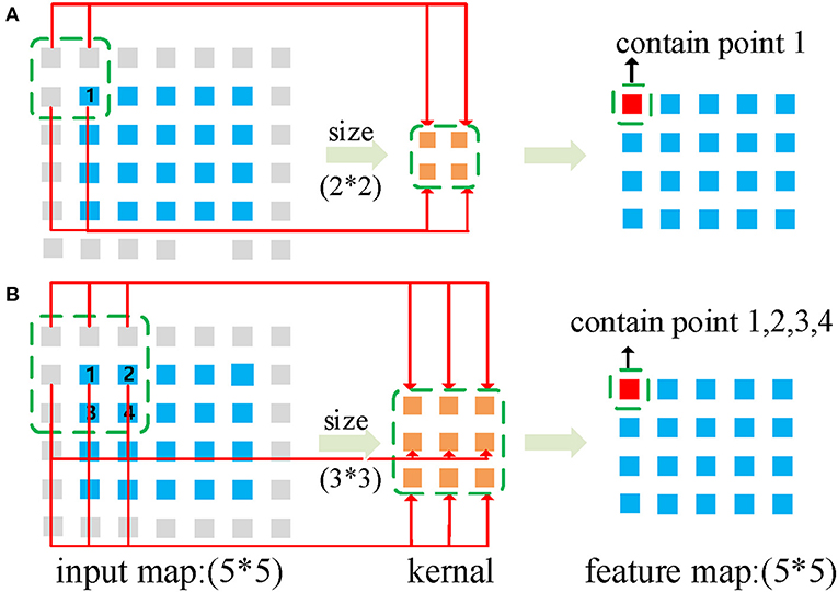
Figure 1. Receptive field: same input and different convolutional kernel. The gray squares represent the padding. (A,B) illustrate how the input map converts the output (feature map) through a convolution operation with 2 × 2 and 3 × 3 kernels, respectively.

The main contributions of this study can, thus, be summarized as follows:

1. We propose a novel framework that uses parallel deep CNNs with a heterogeneous architecture to forecast ENSO. In this study, by replacing the traditional iteration process with parallel predictions, the proposed scheme avoids error accumulation. Meanwhile, with the help of the adaptive selection of heterogeneous neural network architecture, the modeling can be adjusted to accommodate different tasks (lead times) and, thus, improve the reliability of long-term predictions.

2. We investigate and formulate the relationship between different prediction tasks (lead times) and neural network architectures from a unique perspective, namely, the receptive field from computer vision. We discover that with lead time lengthened, the correlated spatial area should be appropriately increased. From the view of computer vision, the prediction spatial-temporal correlated area is corresponding to the receptive field range, which is determined by the convolution kernels size and sampling mesh size of the input in a deep neural network. According to this, we design an adaptive network structure selection method with respect to lead time lengthened and applied it in the long-term ENSO prediction.

3. We validate the effectiveness of the proposed method by comparing its results with those of current efficient methods. The experimental results demonstrate the advantages of the proposed approach.

2. Data and Method

2.1. Data

Since ENSO is related to sea temperature, the monthly SST and heat content (HC) (vertically averaged oceanic temperature in the upper 300 m) anomaly maps are used as two input predictors. The heat exchange in the ocean is carried out by vertical vortex motion, convective mixing, and vertical ocean current convey, so SST and HC are correlated to each other at different moments. The anomaly maps extend over 0°–360°E, 55°S–60°N, and the spatial resolution is 5° latitudes by 5° longitudes.

The dataset used in this study was originally published by Ham et al. (2019). Since the observation data of global oceanic temperature distribution is only available as of 1,871 (Giese and Ray, 2011), only 146 are available for each calendar month. To overcome the limitation, Ham et al. (2019) introduced the Coupled Model Intercomparison Project phase 5 (CMIP5) output to increase the number of samples. The CMIP5 output is the simulation data from the numerical climate model that contains the variables SST and heat content. Therefore, the dataset consists of three-part data (as shown in Table 1): the historical numerical simulations produced by the 21 CMIP5 models (Taylor et al., 2012), the reanalysis data from the Simple Ocean Data Assimilation (SODA) (Giese and Ray, 2011), and the Global Ocean Data Assimilation System (GODAS) (Behringer and Xue, 2004).

TABLE 1

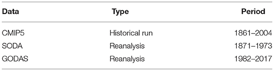
Table 1. The dataset for training and testing the model.

2.2. Receptive Field of CNN

2.2.1. The Size of Receptive Field

Convolutional neural networks have the powerful ability to hierarchically capture spatial structural information (LeCun et al., 1998). They can map the effect of neighborhood points on the center point through a convolution filter and, multilevel convolution processing, they can map the evolution of dynamic complexity between points. The convolution process of CNNs extracts local characteristics from the global maps and calculates dot products between values in the convolution filter and those in the input layer. The jth feature map in the ith convolution layer at grid point (x, y) is calculated by using

$\begin{array}{ll}{v}_{i,j}^{x,y}=tanh\left({\displaystyle \sum _{m=1}^{M_{i-1}}}{\displaystyle \sum _{p=1}^{P_i}}{\displaystyle \sum _{q=1}^{Q_i}}{w}_{i,j}^{p,q}{v}_{(i-1),m}^{(x+p-\frac{P_i}{2},y+q-\frac{Q_i}{2})}+b_{i,j}\right),& (1)\end{array}$

where the hyperbolic tangent serves as the activation function, P_i and Q_i are horizontal and vertical size of the convolution filter for convolution layer i, M_i−1 is the number of feature maps in layer i − 1, $w_{i,j}^{p,q}$ is the weight at grid point (p, q), $v_{(i-1),m}^{(x+p-P_i/2,y+q-Q_i/2)}$ is the value of feature map m for convolution layer i − 1 at grid point (x + p − P_i/2, y + q − Q_i/2), and b_i,j is the bias of feature map j in convolution layer i.

In computer vision, the receptive field represents the spatial mapping of each point after multilevel convolution operations; that is, the size of the receptive field represents the ability to acquire the spatial correlation range, as shown in Figure 1. Figures 1A,B illustrate how the input map converts the output (feature map) through a convolution operation with 2 × 2 and 3 × 3 kernels, respectively, so the receptive field of 1 unit in output is a region containing 4 units in the input map in Figure 1A, whereas it contains 9 units in Figure 1B. Given a deep CNN, the receptive field term usually considers the final output unit in relation to the network input. For example, as shown in Figure 2, the receptive field of the unit in the final output map denotes the area in the input map, which consists of every unit that has propagated its value through the whole chain to the given end unit.

FIGURE 2

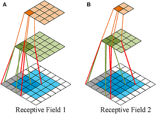
Figure 2. Receptive field a deep CNN. (A) The first convolving: a 3 × 3 kernel over a 5 × 5 input padded with a 1 × 1 border of zeros using unit strides. The second convolving: a 2 × 2 kernel using unit strides. (B) The first convolving: a 4 × 4 kernel over a 5 × 5 input padded with a 1 × 1 border of zeros using unit strides. The second convolving: a 2 × 2 kernel using 2 × 2 strides.

It is easy to calculate the size of the receptive field of an output unit in a basic CNN with a fixed structure, since only the convolution and pooling layers can affect its size. The convolution layer uses the kernel to execute the convolution operation to multiply the receptive distance by the kernel size. The pooling layer downsamples following a certain stride to multiply the receptive distance by stride size. Thus, the receptive field size can be formulated as

$\begin{array}{ll}R{F}_{i+1}=R{F}_i+(K_{\text{size}i+1}-1)S_i,& (2)\end{array}$

where RF_i+1 and RF_i are the receptive field of layers (i + 1) and (i), respectively, with RF₀ = 1, S_i is the product of all layer strides before layer (i + 1) (i.e., $S_i={\prod }_{i=1}^i{\text{Stride}}_i$), and K_sizei+1 is the size of convolution kernels at layer (i + 1). Thus, the receptive field area of the last feature map on the input image is (RF_n, RF_n), where n is the last convolution layer in the network.

Note that Equation (2) is calculated based on the assumption that the shape of input images and convolution kernels are square, whereas the input anomaly maps and convolution in the model are rectangular, so Equation (2) must be rewritten as

$\begin{array}{l}R{F}_i=(R{F}_i^x,R{F}_i^y)\end{array}$

$\begin{array}{l}R{F}_{i+1}=R{F}_i+(P_{i+1}-1)\times S_i\end{array}$

$\begin{array}{ll}R{F}_{i+1}=R{F}_i+(Q_{i+1}-1)\times S_i& (3)\end{array}$

where the receptive field area of the last feature map on the input image is $(R{F}_n^x,R{F}_n^y)$.

2.2.2. Relationship Between Receptive Field and Lead Time

In the simulated prediction, each grid point in the input is spatio-temporally correlated. Specifically, owing to the complicated interactions of the global climate system, the one grid point is highly correlated to the near points and distant points, and hence the slight changes of grid point will lead to the variation of other points. Therefore, in this study, the spatio-temporal correlated area can be regarded as the receptive field in CNN.

All related works applied only a single DL model for multi year ENSO forecasts, which use the same size of convolution kernels and the same step size for different lead times. Therefore, according to Equation (2), the receptive field is the same for different lead times. However, with the increase of prediction lead times, the spatio-temporal correlated area of each point differs. Sønderby et al. (2020) used 64 km as the basic unit to predict the probability of precipitation in the next 8 h. With an input patch covering 1,024 × 1, 024 km and an average precipitation displacement of 1 km per min, they set the target patch to cover 64 × 64 km centered on the input patch. They mentioned that accurate predictions of the target tensor for a longer lead time require a larger spatio-temporal context around the target. Therefore, in the prediction problem, the spatio-temporal correlated area (receptive field) of the target should expand with the increase of lead time. As mentioned, the receptive field size is determined by the stride size and the size of the convolution kernels. To this end, we now design a scheme by adjusting the two parameters to appropriately expand the receptive field size.

First, the input mesh size can be selected by changing the stride size through multiple pooling processes. The mesh size of the input means the receptive field resolution; that is, each input grid point represents the number of original grid points. The increase in receptive field resolution allows not only the small range simulations and noises to be smoothed but also the receptive field to be expanded. We assume that the receptive field resolution should increase by a multiple of four as the prediction lead time increases. In prediction modeling, the predicted lead times are divided into three stages for ENSO forecasts: short, medium, and long term, which can be stated as

$\begin{array}{ll}{T}_{\text{term}}=\{\begin{array}{c}\text{Short term (ST)},\\ \text{Medium term (MT)},\\ \text{Long term (LT)},\end{array}\begin{array}{c}\frac{\left|lt\right|-1}{5}\le 1\\ 1<\frac{\left|lt\right|-1}{5}\le 3\\ 3<\frac{\left|lt\right|-1}{5},\end{array}& (4)\end{array}$

where lt is the lead time of ENSO forecasts, which ranges from 1 to 20 months. Thus, the receptive field resolution for these three terms is 1 : 4 : 16.

The mesh size of the original image is changed and, with the increased lead time, the receptive field is enlarged at the first assumption. However, in computer vision, a larger receptive field does not mean better performance. Luo et al. (2016) also refer to the concept of an effective receptive field. Increasing the mesh size causes the receptive field to expand fourfold, so it is slightly larger.

Second, in the process of convolution feature extraction, we change the kernel size to adjust the size of the expanding receptive field. We assume that the receptive field enlarges at the rate of 2α^N−1 (0 < α ≤ 1) with the increase of lead term; N represents T_term and its value is 1, 2, 3 for each of these three terms. In conclusion, we formulate the relationship between the prediction lead time, input mesh size, and kernel size to increase the receptive field and realize multi-task modeling of spatio-temporal differences.

2.3. Architecture Details

Given that the same single model for multi year ENSO forecast is often unreliable and more difficult to train (Chevillon, 2007; Shi and Yeung, 2018), a more promising strategy must be proposed for long-term prediction. Thus, considering the differences in the spatio-temporal dependencies of different tasks, we propose a framework that uses parallel deep CNNs with heterogeneous architectures to forecast ENSO. Figure 3 illustrates the schematic structure of the framework, which is called the MS-CNN model and consists of four parts: the input mesh size selection (IMSS) module, the multiterm swappable convolution (MSC) module, the fully connected (FC) module, and the parallel prediction result splicing (PPRS) module.

FIGURE 3

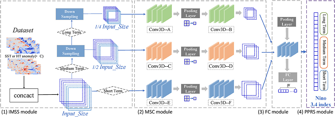
Figure 3. The architecture of the MS_CNN model. (1) Input mesh size selection (IMSS) module aims to increase the input mesh size as the prediction lead time lengthened. (2) Multi-term swappable convolution (MSC) module is mainly to adjust the appropriate receptive field expansion. (3) Fully connected (FC) module transforms the feature map of CNN to vector, and then output the prediction of Nino 3.4 index. (4) Parallel prediction result splicing (PPRS) module splices the Nino 3.4 index of each lead time at the parallel network.

The IMSS module automatically selects different sampling mechanisms according to the three prediction terms. The sampling mechanism changes the mesh size of the input by selecting the pooling strategy to increase the receptive field. The hypothesis that the resolution of the receptive field should increase with prediction time is realized by the subsampling mechanism. SST and HC anomaly maps for three consecutive months serve as original input predictors.

In the MSC module, we set up a heterogeneous network architecture to select one model of these three-term periods adaptively based on the CNN network model (Ham et al., 2019). This module serves mainly to adjust the expanding receptive field of the first module by setting the size of the convolution kernels to appropriately expand the receptive field. In the proposed model, before the feature map enters the fully connected layer of the FC module, the process after downsampling is convolution → pool → convolution → pool → convolution. We assume that the three convolutions have sizes (P₁, Q₁), (P₂, Q₂), (P₃, Q₃), so the receptive field of these three terms is

$\begin{array}{ll}RF=4^s((4P_3+2P_2+P_1-3),(4Q_3+2Q_2+Q_1-3)),& (5)\end{array}$

where s represents the different downsampling scales of the three terms, with s = 0 for ST, s = 1 for MT, and s = 2 for LT.

To satisfy the above assumption that the receptive field grows at the rate of 2α^N−1 (0 < α ≤ 1) with respect to the increase in the prediction lead time, the receptive field should grow appropriately for different lead terms. Therefore, we formulate the relationships between input mesh size (downsampling strategy), convolution kernel size, and the time period in the network to control the size of the receptive field under these three terms and improve the accuracy of prediction. The formula is

$\begin{array}{ll}(C_1,C_2)=(P_3{P}_2{P}_1,Q_3{Q}_2{Q}_1){\displaystyle \prod _{m=1}^s}{2}^{(m-1)},& (6)\end{array}$

where s is the same as in Equation (5), C₁ and C₂ are the same constants for the three terms in the model. We control the receptive field by adjusting C₁ and C₂ and use the large convolution kernels for the short term and the small convolution kernels for the long term to make the product (6) a constant.

The FC module transforms the CNN feature map to a vector and then outputs the prediction of the Niño 3.4 index. The PPRS module is used to splice Niño 3.4 index of each lead time at the parallel network, and the final result is the prediction of the whole lead time series. In this study, by replacing a traditional iteration with the same model with parallel prediction, the proposed scheme avoids error accumulation. Thus, by designing the heterogeneous architecture model, the evolution of different lead times can be fully explored.

3. Experiments

We ran the numerical experiments on a single NVIDIA RTX2080ti-11G, and the proposed model was implemented by using Python 3.6 with Pytorch.

3.1. Experiment Settings

a) Input and output data: Sea surface temperature and HC anomaly maps are used as inputs. The output of the model is the Nino 3.4 index, which is the area-averaged SST anomaly over the Nino3.4 region, as a predictand to be predicted up to 20-months-ahead. That is, only SST is used to calculate the actual result of the Nino3.4 index. HC is just an additional input predictor. More specifically, the model uses SST and HC for three consecutive months as input, so the input size is 6 × 72 × 24 (an anomaly map size is 72 × 24). A single network output is the predicted value of the Nino3.4 index for the corresponding lead month, so the size is 1 × 1. The final output of the parallel networks is a 20 × 1 vector of Nino3.4 index from 1- to 20-month-lead. The transfer learning technique is used to optimally train the model. The SODA of 1871–1973 is used for the training period to minimize the systematic errors caused by the CMIP5 samples (from 1861 to 2004). Then, we use the GODAS of 1982–2017 for testing the forecast skill of the model.

b) Evaluation metrics: To evaluate the performance of the MS-CNN model, we adopt two commonly used metrics such as Temporal Anomaly Correlation Coefficient Skill (Corr) and Root Mean Square Error (RMSE) of the prediction lead months. Corr measures the linear correlation between the predicted value and the actual value, whereas the RMSE measures the difference. The formulas for calculating the Corr and RMSE are

$\begin{array}{ll}Cor{r}_l={\displaystyle \sum _{m=1}^{12}}\frac{{\displaystyle {\sum }_{t=s}^e}(Y_{t,m}-{Ȳ}_m)(P_{t.m.l}-{\bar{P}}_{m,l})}{\sqrt{{\displaystyle {\sum }_{t=s}^e}{(Y_{t,m}-{Ȳ}_m)}^2{\displaystyle {\sum }_{t=s}^e}{(P_{t.m.l}-{\bar{P}}_{m,l})}^2}}& (7)\end{array}$

$\begin{array}{ll}RMS{E}_l={\displaystyle \sum _{m=1}^{12}}\sqrt{\frac{{\displaystyle {\sum }_{t=s}^e}{(Y_{t,m}-P_{y·m.l})}^2}{|e-s|}}& (8)\end{array}$

where P and Y are the predicted value and observed value, respectively, ${\bar{P}}_{m,l}$ and Ȳ_m are the mean values of P and Y, m = 1–12 is the calendar month, the label t is the forecast target year, and s = 1982 and e = 2017 are the starting and ending years, respectively.

3.2. Comparison of Different MS-CNN Structures

To further analyze the relationships between the different network structures and simulation results and to prove that the proposed model is reasonable, we compare it with three aspects of the MS-CNN model: (1) the number of layers, which is a fundamental setting for deep neural-network structure; (2) the size of the region on original maps, which is the geographic scope of the original area; and (3) the relationship between the three terms, the size of the input mesh, and the size of the convolution kernel, which represent the change in receptive field size as the lead time lengthens. Experiments (1) and (2) were implemented on the same parallel model based on CNNs to select the optimal basic parameters for the subsequent Experiment (3).

Tables 2, 3 show the comparison of Corr and RMSE between different layers. The results show that, (1) at each layer, both metrics deteriorate as the lead time increases, and (2) more layers do not always guarantee better performance. It is observed that the RMSE of the results decreases at the outset and then increases over the next few lead months. Previous experiments (Mu et al., 2019) show that implementing more layers does not improve performance, because of insufficient training data for a large number of parameters. In this experiment, three layers can be considered as an appropriate choice under the two metrics.

TABLE 2

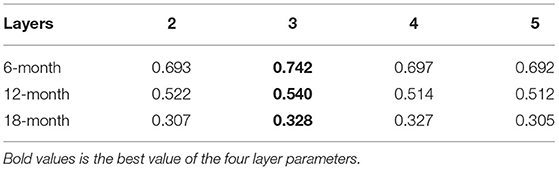
Table 2. Correlation skill (Corr) of lead times with different layers.

TABLE 3

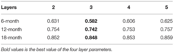
Table 3. Root Mean Square Error (RMSE) of lead times with different layers.

Next, Figures 4, 5 show the performance of different original anomaly maps with a three-layer network. In these figures, areas 1, 2, 3, and 4 represent the Nino3.4 region(5°S–5°N, 170°W–100°W), (15°S–15°N, 170°E–100°W), (30°S–30°N, 125°E–55°W), (55°S–60°N, and 0°E–360°E), respectively. The existing DL models for ENSO forecasting use mostly the Nino3.4 area as original input, but Park mentioned that SST anomalies outside the equatorial Pacific Ocean can lead to an ENSO event with a time-lag longer than 1 year (Park et al., 2018). Therefore, we explore how the region size of original anomaly maps affects multi year forecasts. The results show that (1) at each region, both metrics deteriorate as the lead time increases, and (2) larger original anomaly maps result in more accurate forecasting. These results show that the SST patterns are related to each other over a vast area of the ocean, which is consistent with the opinion of Park. We, thus, choose the entire anomaly maps (55°S–60°N, 0°E–360°E) as the original maps.

FIGURE 4

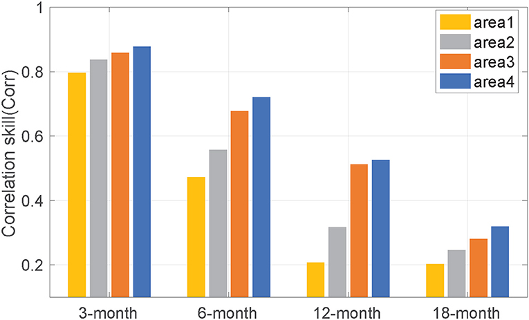
Figure 4. The correlation skill (Corr) between predicted values and actual values with different input sizes. The different input size represents the different regional ranges: area1 (yellow) represents the Nino3.4 region (5°S–5°N, 170°W–120°W), area2 (gray) represents the region of (15°S–15°N, 170°E–100°W), area3 (orange) represents the region of (30°S–30°N, 125°E–55°W), and area4 (blue) represents the region of (55°S–60°N, 0°E–360°E).

FIGURE 5

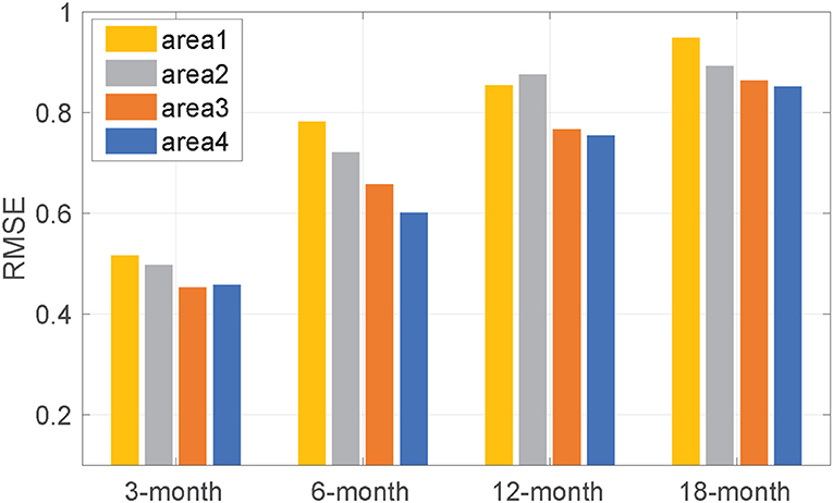
Figure 5. Root Mean Square Error between predicted values and actual values with different input sizes. Refer to Figure 4 for the information of the area1, 2, 3, 4.

With the fixed layer and original map area, we next explore the relationship between lead time, input mesh size, and the size of the convolution kernels to determine how the receptive field changes to improve the reliability of ENSO predictions as the lead time increases. Figures 6, 7 show that single-scale means that the original map does not downsample for any of these three lead terms. In the same way as with the MSC module, the sizes of the convolution kernels for the three lead terms are all the same [A/C/E (8,4) and B/D/F (4,2)]. Thus, the receptive field size about these three terms has a ratio of 1:1:1. Multis cale (1) means that lead times are divided into three terms, and these three terms correspond to the different mesh size of the input map by downsampling. The relationship between the three terms, the mesh size, and the size of the convolution kernel is consistent with Equation (6): C1 = 64 and C2 = 16, the Conv3d is A(8,4), B/C/D (4,2), E/F (2,1), so the size of the receptive field about these three terms has the approximate ratio of 1:2.5:4. Multiscale (2) is similar to multiscale (1), but the relationship is not consistent with Equation (6). Instead, it uses the same Conv3d [A/C/E (8,4), B/D/F (4,2)] in the MSC module, so the size of the receptive field about these three terms has a ratio of 1:4:16. We can observe from Figures 6, 7, both Corr and RMSE, the multi scale (1) scheme corresponding to Equations (5) and (6) perform best. The receptive field nearly expands at the rate of 2α^N−1 (α = 1) for three terms. Moreover, with increasing lead time, the performance gap between the three terms increases. The single-scale scheme does not build different receptive field models to differentiate spatio-temporal dependencies. Multi scale (2) scheme expands the receptive field indefinitely. This scheme only expands the receptive field resolution but does not change the kernel size to adjust the receptive field. Neither of these two schemes fits the hypothesis, and the ratio does not expand at the rate of 2^N−1 for these three terms. These results prove that the hypothesis is correct and that the method to appropriately expand the receptive field size is reasonable.

FIGURE 6

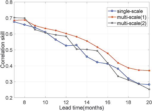
Figure 6. The Corr between predicted values and actual values with different relationships among lead months, input mesh size, and convolution kernel size. Their relationship determines the ratio of the receptive field size in the three prediction lead terms. Single-scale means that input mesh size and convolution kernel size are the same with the increase of lead months. The Conv3d are A/C/E (8,4), B/D/F (4,2) at MSC module. Thus, the receptive field size about these three terms has a ratio of 1:1:1. Multi scale(1) means their relationship is consistent with Equation (6). Noticeably, these three terms correspond to the different input mesh size by downsampling the original map and the ratio of input mesh size is 1:4:16. The Conv3d are different at MSC module, is A(8,4)/B(4,2),C/D (4,2), E/F (2,1). So the receptive field size about these three terms has an approximate ratio of 1:2.5:4. Multi scale(2) have the same input mesh size as multi scale(1) in these three lead terms. But multi scale(2) uses the same Conv3d (A/C/E (8,4), B/D/F (4,2)) at MSC module, so the relationship is not consistent with Equation (6). The size of the receptive field about these three terms has a ratio of 1:4:16.

FIGURE 7

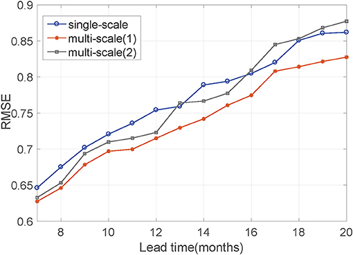
Figure 7. Root Mean Square Error between predicted values and actual values with different relationships among lead months, input mesh size, and convolution kernel size. Their relationship determines the ratio of the receptive field size in the three prediction stages. Refer to Figure 6 for the information on the single-scale, multi scale (1), and multi scale (2).

3.3. Performance Comparison of Different Models

We now compare the MS-CNN model with the following SST prediction models and multiscale models of computer vision:

a. The method of Ham et al. (2019). A multi year ENSO forecast model based on CNNs and denoted HAM-CNN. The parallel model is formulated separately for each forecast lead month and target season.

b. The method of Zheng et al. (2020). A model with four stacked composite layers for forecasting the evolution of the SST. It is denoted ZG-PSDL.

c. UNET (Ronneberger et al., 2015). A multiscale model for image segmentation. The features of different scales are extracted by using downsampling, and then the output of upsampling is combined with feature maps of the corresponding scale to the decoder.

d. LSTM-FC (Zhao et al., 2019). An LSTM model with a FC neural network.

The deep neural networks are trained with the same number of epochs for a meaningful comparison: 80 epochs are used for the first training using the CMIP5 output, and 30 epochs are used for the second training using the reanalysis data. The total number of convolution filters is 30. An Adam optimizer is applied during the training process. The size of the mini-batch for each epoch is set to 64, and the learning rate is fixed to 0.005.

Inspired by Ham et al. (2019), Figure 8 facilitates the comparison. Figure 8A shows the all-season Corr of the 3-month moving-averaged Niño3.4 index from 1982 to 2017. We experiment with forecasting 1–20 months in advance, and the forecast accuracy of the Niño3.4 index in the MS-CNN model is systematically superior to that of the other models, especially for lead times longer than 6 months. The all-season Corr of the Niño3.4 index in the MS-CNN model is greater than 0.50 for up to a lead time of 16 months, whereas it is 0.41 for a lead time of 16 months in the HAM-CNN model. The HAM-CNN model provides accurate predictions, but when we introduce multiscale network architecture and the method of adaptively controlling the size of convolution kernels to enlarge the receptive field (that is, the MS-CNN model), the prediction accuracy significantly improves for medium to long lead times.

FIGURE 8

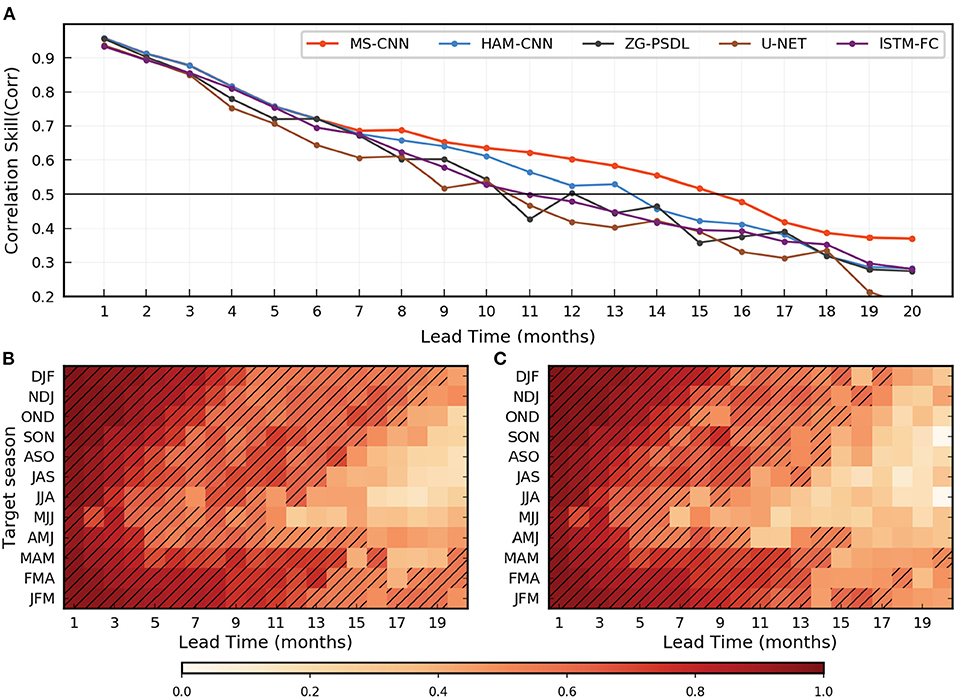
Figure 8. Multi year El Nino-Southern Oscillation (ENSO) forecasts Corr in the MS-CNN model. (A) The all-season correlation skill of the 3-month-moving-averaged Nino3.4 index as a function of the forecast lead month in the model (red), HAM-CNN model (blue), ZG-PSDL(black), and U-net model(brown). (B,C) The correlation skill of the Nino3.4 index targeted to each calendar month in the MS-CNN model (B) and the HAM-CNN model (C). Hatching highlights the forecasts with correlation skills exceeding 0.5.

Zhenggang's model and UNET use a multiscale model, but both models have the same convolution kernels for different lead times, which prevents them from controlling the size of receptive fields. Moreover, both models are fused multiscale feature maps, which introduce noise so that the results fluctuate badly. Therefore, we conclude that the MS-CNN model provides a skillful and stable forecast of ENSO phenomena for up to a lead time of 18 months.

The MS-CNN model also provides a greater Corr than the HAM-CNN model for the Niño3.4 index for almost each target season (as shown in Figures 8B,C). The improvement in Corr is clear at longer lead times and is robust for target seasons between the late boreal spring and autumn. For example, the forecasts for the May-June-July season have a correlation skill exceeding 0.50 up to lead time of 10 months for the MS-CNN model, but only up to a lead time of 6 months for the HAM-CNN model. In addition, for the HAM-CNN model, the Corr fluctuates significantly for medium lead time (11–16 months), but the result of the model is relatively stable and decreases for longer lead times. This narrows the gap in the ability of the proposed model to forecast different target seasons. The conclusion imposed is that the MS-CNN model is robust and essentially independent of the spring predictability barriers.

3.4. Results of the MS-CNN Model

Considering the heat exchange in the ocean, we analyze the influence of SST and HC on the prediction results. Figure 9 shows the performance of different input predictors with CNN and the MS-CNN model. The results show that: (1) the Corr of only SST is higher than only HC, which confirms that SST is the most important factor. The reason is that the Nino3.4 index is obtained by calculating the area-averaged SST anomaly over the Nino3.4 region, so the input of SST is the key factor that decides the fluctuation of results; (2) SST+HC scheme both perform best on CNN and MS-CNN model. These results indicate although the predicted Nino3.4 index is only related to SST, the HC as an input predictor can significantly improve the accuracy of long-term prediction. The reason is that internal ocean motion, such as vertical vortex motion and convective mixing, produces heat exchange. To be more specific, the ocean under the surface can transfer heat to the ocean surface for a while, and vice versa. Therefore, using SST and HC for several previous months as two input predictors, the model can extract some laws and features of ocean internal motion for better long-term prediction.

FIGURE 9

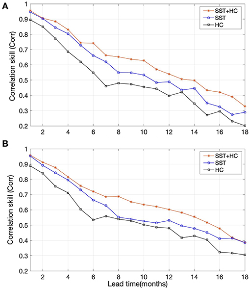
Figure 9. The Corr between predicted values and actual values with different input predictors based on (A) CNN model, (B) MS-CNN model. The red line shows SST and heat content (HC) were all used as input predictors. The blue line shows only SST was used as input predictors. The black line shows only HC was used as input predictors.

We regarded the spatio-temporal correlated area as the receptive field in the study. Given the complicated interactions of the global climate, each grid point is highly correlated to near points and distant points, so slight changes of a grid point will cause other points to vary. For short-term forecasting, a small correlated area is enough to predict the change of the grid point. But for long-term forecasting, a larger correlated area should be used. First, we smooth out the fluctuations and noise by changing the mesh size and then adjust the receptive field by changing the convolution kernel size. The correlation can be extracted from the convolution kernel of CNN. We make the physical assumption that as the prediction lead time increases, the space temporal correlated area of each grid point should increase appropriately, that is, the receptive field of a pixel in CNN last layer should increase appropriately. More specifically, we assume that the receptive field enlarges at the rate of 2α^N−1 (0 < α ≤ 1) with respect to the increase in the leading term. Figure 6 shows that the assumption is reasonable and its performance is best in these three schemes. The traditional method did not consider the dynamic variation that the spatio-temporal correlated area of grid point will change as the prediction lead time increases. The single-scale scheme, which is the traditional method of using only a single model for all lead times, does not build different receptive field models to differentiate spatio-temporal dependencies. The multi scale (2) scheme, which only expands the receptive field resolution by downsampling, does not change the kernel size to adjust the receptive field and lead to the receptive field expand indefinitely. Therefore, the physical assumption that as the prediction lead time increases, the spatio-temporal correlated area of each grid point should increase appropriately is correct.

The Nino3.4 index from 1982 to 2017 was predicted 1–20 months in advance in this experiment. The result from Figure 8A shows that the 1-month-lead prediction is the most accurate, and the 20-month-lead prediction is the least accurate. Specifically, the curve produced by the 1-month-lead prediction of Corr is 0.96, and the corresponding RMSE is 0.31; the Corr predictions with a 16-month lead are all greater than 0.50; even for the 20-month-lead prediction, the worst Corr approaches 0.40, and the corresponding RMSE is 0.83. As shown in Figure 8B, the MS-CNN model generally provides accurate predictions for autumn and winter (e.g., for December, January, and February, Corr is greater than 0.50 for 19 consecutive months). Although the results for spring and summer are improved compared with other models, the prediction results remain poor in the medium and long term.

The Niño3.4 index for the January-February-March season for 1-, 6-, 12-, and 18-month-lead predictions demonstrates that the proposed MS-CNN model predicts the evolution and the ENSO amplitude by the 12-month-lead time (Figure 10). The Corr values are 0.96, 0.87, 0.68, and 0.60, respectively. However, at times with strong EI Niño or La Niña phenomena, the prediction errors become relatively large with increasing lead time. Thus, the proposed method is better than previous methods but does not work well for longer lead times in a more demanding environment.

FIGURE 10

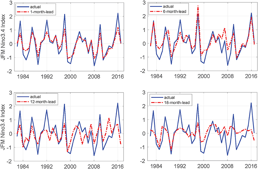
Figure 10. Predicted and actual values of the January-February-March season Nino3.4 indexes for four different lead months.

4. Conclusion

Improving the predictability of ENSO is the key to better seasonal predictions across the globe. At present, the DL-based methods for multi year ENSO forecasts only focus on the application of deep neural networks, but none consider the distribution characteristics of oceanic spatio-temporal data. Using SST and HC for several previous months as two input predictors, the model can extract some laws and features of ocean internal motion for better long-term prediction. It can be concluded that it is feasible to improve the reliability of the long-term prediction by adding more related predictors as input.

The spatio-temporal correlated area was regarded as the receptive field in this study. We make the physical assumption that the space-temporal correlated area of each grid point should increase appropriately with the lead time increases, that is, the receptive field of a pixel in CNN last layer should increase appropriately. Given the differences in the spatio-temporal dependencies of different lead times for forecasting ENSO, we build a framework that we call the ”MS-CNN model” by using parallel deep CNN with a heterogeneous architecture for multi year ENSO forecasts. First, by replacing the traditional iteration process with parallel predictions, the proposed scheme avoids error accumulation. Second, by using an adaptive selection of heterogeneous neural network architectures, we adaptively expand the receptive field with increasing prediction lead time. The results of using the model on a real-world dataset show that the hypothesis (i.e., the receptive field expands appropriately as the prediction lead time increases) is reasonable. The reanalysis data for 1982–2017 were predicted 1–20 months in advance. Furthermore, the proposed method provides more accurate predictions than other models, especially for a longer lead times: the Corr is nearly 0.60 for 13-month-ahead and 0.40 for 18-month-ahead.

Although the method proposed for multi year ENSO forecasts significantly improves upon the performance of the conventional methods, some shortcomings remain. For instance, when strong ENSO events happen, the prediction of the Niño3.4 index is relatively inaccurate, and the errors increase with increasing prediction lead time. In addition, the predictions are more accurate than those of other models only for spring, as opposed to all seasons. Thus, in future research, we will focus on the following three themes: (1) introducing more related measurements, such as westerly wind bursts and warm water volume, to model the spatio-temporal process more comprehensively and improve ENSO forecasting for the spring season; (2) integrating the CONVLSTM with the proposed method to determine whether it is generalizable and whether it can further improve the accuracy of multi year ENSO forecasts; (3) learning more knowledge in the marine field and improving the reliability of forecasting by combining the DL methods with numerical simulation models.

Data Availability Statement

Publicly available datasets were analysed in this study. This data can be found here: Ham et al. (2019), https://doi.org/10.5281/zenodo.3244463.

Author Contributions

MY performed methodology, data processing, modeling, and writing of the original draft. ZWe performed validation and review. LH, HT, and DS performed validation and investigation. AL and ZWa optimized the model framework. JN contributed to conceptualization, writing review and editing, and supervision. All authors contributed to the article and approved the submitted version.

Funding

This study was supported in part by the National Natural Science Foundation of China (62072418), the Fundamental Research Funds for the Central Universities (202042008), and the Major Scientific and Technological Innovation Project (2019JZZY020705).

Conflict of Interest

The authors declare that the research was conducted in the absence of any commercial or financial relationships that could be construed as a potential conflict of interest.

Publisher's Note

All claims expressed in this article are solely those of the authors and do not necessarily represent those of their affiliated organizations, or those of the publisher, the editors and the reviewers. Any product that may be evaluated in this article, or claim that may be made by its manufacturer, is not guaranteed or endorsed by the publisher.

References

Behringer, D., and Xue, Y. (2004). “Evaluation of the global ocean data assimilation system at ncep: the Pacific ocean,” in 24th Conference on Integrated Observing and Assimilation Systems for the Atmosphere, Oceans, and Land Surface (IOAS-AOLS). Seattle, WA.

Google Scholar

Broni-Bedaiko, C., Katsriku, F. A., Unemi, T., Atsumi, M., Abdulai, J.-D., Shinomiya, N., and Owusu, E. (2019). El ni no-southern oscillation forecasting using complex networks analysis of lstm neural networks. Arti. Life Rob. 24, 445–451. doi: 10.1007/s10015-019-00540-2

CrossRef Full Text | Google Scholar

Cane, M. A., Zebiak, S. E., and Dolan, S. C. (1986). Experimental forecasts of el nino. Nature 321, 827–832. doi: 10.1038/321827a0

CrossRef Full Text | Google Scholar

Chevillon, G. (2007). Direct multi-step estimation and forecasting. J. Econ. Surv. 21, 746–785. doi: 10.1111/j.1467-6419.2007.00518.x

CrossRef Full Text | Google Scholar

Duan, W., and Wei, C. (2013). The ' spring predictability barrier' or enso predictions and its possible mechanism: results from a fully coupled model. Int. J. Climatol. 33, 1280–1292. doi: 10.1002/joc.3513

CrossRef Full Text | Google Scholar

Forootan, E., Awange, J. L., Schumacher, M., Anyah, R., van Dijk, A. I., Kusche, J., et al. (2016). Quantifying the impacts of enso and iod on rain gauge and remotely sensed precipitation products over australia. Remote Sens Environ. 172, 50–66. doi: 10.1016/j.rse.2015.10.027

CrossRef Full Text | Google Scholar

Gál, V., Hámori, J., Roska, T., Bálya, D., Borostyánkői, Z., Brendel, M., et al. (2004). Receptive field atlas and related cnn models. Int. J. Bifurcat. Chaos 14, 551–584. doi: 10.1142/S0218127404009545

CrossRef Full Text | Google Scholar

Giese, B. S., and Ray, S. (2011). El ni no variability in simple ocean data assimilation (soda), 1871-2008. J. Geophys. Res. Oceans 116:C02024. doi: 10.1029/2010JC006695

CrossRef Full Text | Google Scholar

Goddard, L., Mason, S. J., Zebiak, S. E., Ropelewski, C. F., Basher, R., and Cane, M. A. (2001). Current approaches to seasonal to interannual climate predictions. Int. J. Climatol. 21, 1111–1152. doi: 10.1002/joc.636

CrossRef Full Text | Google Scholar

Gupta, M., Kodamana, H., and Sandeep, S. (2020). Prediction of enso beyond spring predictability barrier using deep convolutional lstm networks. IEEE Geosci. Remote Sens. Lett. 1–5. doi: 10.1109/LGRS.2020.3032353

CrossRef Full Text | Google Scholar

Ham, Y.-G., Kim, J.-H., and Luo, J.-J. (2019). Deep learning for multi-year enso forecasts. Nature 573, 568–572. doi: 10.1038/s41586-019-1559-7

PubMed Abstract | CrossRef Full Text | Google Scholar

He, D., Lin, P., Liu, H., Ding, L., and Jiang, J. (2019). “Dlenso: a deep learning enso forecasting model,” in Pacific Rim International Conference on Artificial Intelligence (Cuvu: Springer), 12–23.

Google Scholar

LeCun, Y., Bottou, L., Bengio, Y., and Haffner, P. (1998). Gradient-based learning applied to document recognition. Proc. IEEE 86, 2278–2324. doi: 10.1109/5.726791

CrossRef Full Text | Google Scholar

Luo, W., Li, Y., Urtasun, R., and Zemel, R. (2016). “Understanding the effective receptive field in deep convolutional neural networks,” in Proceedings of the 30th International Conference on Neural Information Processing Systems (Barcelona), 4905–4913.

Google Scholar

Masumoto, Y., Sasaki, H., Kagimoto, T., Komori, N., Ishida, A., Sasai, Y., et al. (2004). A fifty-year eddy-resolving simulation of the world ocean: preliminary outcomes of OFES (OGCM for the Earth Simulator). J. Earth Simul. 1, 35–56.

Google Scholar

Mcdermott, P. L., and Wikle, C. K. (2017). An ensemble quadratic echo state network for non-linear spatio-temporal forecasting. Stat 6, 315–330. doi: 10.1002/sta4.160

CrossRef Full Text | Google Scholar

Mu, B., Peng, C., Yuan, S., and Chen, L. (2019). “Enso forecasting over multiple time horizons using convlstm network and rolling mechanism,” in 2019 International Joint Conference on Neural Networks (IJCNN) (Budapest: IEEE), 1–8.

Google Scholar

Park, J.-H., Kug, J.-S., Li, T., and Behera, S. K. (2018). Predicting el ni no beyond 1-year lead: effect of the western hemisphere warm pool. Sci. Rep. 8, 1–8. doi: 10.1038/s41598-018-33191-7

PubMed Abstract | CrossRef Full Text | Google Scholar

Ronneberger, O., Fischer, P., and Brox, T. (2015). “U-net: Convolutional networks for biomedical image segmentation,” in International Conference on Medical Image Computing and Computer-Assisted Intervention (Cham: Springer), 234–241.

Google Scholar

Rosmiati, R., Liliasari, S., Tjasyono, B., and Ramalis, T. R. (2021). Development of arima technique in determining the ocean climate prediction skills for pre-service teacher. J. Phys. 1731:012072. doi: 10.1088/1742-6596/1731/1/012072

CrossRef Full Text | Google Scholar

Santoso, A., Mcphaden, M. J., and Cai, W. (2017). The defining characteristics of enso extremes and the strong 2015/2016 el ni no. Rev. Geophys. 55, 1079–1129. doi: 10.1002/2017RG000560

CrossRef Full Text | Google Scholar

Shi, X., and Yeung, D.-Y. (2018). Machine learning for spatio-temporal sequence forecasting: a survey. arXiv preprint arXiv:1808.06865.

Google Scholar

Shukla, R. P., Tripathi, K. C., Pandey, A. C., and Das, I. (2011). Prediction of indian summer monsoon rainfall using nio indices: a neural network approach. Atmos. Res. 102, 99–109. doi: 10.1016/j.atmosres.2011.06.013

CrossRef Full Text | Google Scholar

So, M. K., and Chung, R. S. (2014). Dynamic seasonality in time series. Comput. Stat. Data Anal. 70, 212–226. doi: 10.1016/j.csda.2013.09.010

CrossRef Full Text | Google Scholar

Sønderby, C. K., Espeholt, L., Heek, J., Dehghani, M., Oliver, A., Salimans, T., et al. (2020). Metnet: a neural weather model for precipitation forecasting. arXiv preprint arXiv:2003.12140. Available online at: https://arxiv.org/abs/2003.12140

Google Scholar

Taylor, K. E., Stouffer, R. J., and Meehl, G. A. (2012). An overview of cmip5 and the experiment design. Bull. Am. Meteorol. Soc. 93, 485–498. doi: 10.1175/BAMS-D-11-00094.1

CrossRef Full Text | Google Scholar

Wang, Y., Jiang, J., Zhang, H., Dong, X., Wang, L., Ranjan, R., and Zomaya, A. Y. (2017). A scalable parallel algorithm for atmospheric general circulation models on a multi-core cluster. Future Generation Comput. Syst. 72, 1–10. doi: 10.1016/j.future.2017.02.008

CrossRef Full Text | Google Scholar

Xingjian, S., Chen, Z., Wang, H., Yeung, D.-Y., Wong, W.-K., and Woo, W.-C. (2015). “Convolutional lstm network: a machine learning approach for precipitation nowcasting,” in Advances in Neural Information Processing Systems, Vol. 28, 802–810.

Google Scholar

Yan, J., Mu, L., Wang, L., Ranjan, R., and Zomaya, A. Y. (2020). Temporal convolutional networks for the advance prediction of enso. Sci. Rep. 10, 8055. doi: 10.1038/s41598-020-65070-5

PubMed Abstract | CrossRef Full Text | Google Scholar

Yang, S., Li, Z., Yu, J.-Y., Hu, X., Dong, W., and He, S. (2018). El ni no-southern oscillation and its impact in the changing climate. Natl. Sci. Rev. 5, 840–857. doi: 10.1093/nsr/nwy046

CrossRef Full Text | Google Scholar

Zebiak, S. E., and Cane, M. A. (1987). A model el ni n-southern oscillation. Mon. Weather Rev. 115, 2262–2278. doi: 10.1175/1520-0493(1987)115 <2262:AMENO>2.0.CO;2

CrossRef Full Text | Google Scholar

Zhang, Q., Wang, H., Dong, J., Zhong, G., and Sun, X. (2017). Prediction of sea surface temperature using long short-term memory. IEEE Geosci. Remote Sens. Lett. 14, 1745–1749. doi: 10.1109/LGRS.2017.2733548

CrossRef Full Text | Google Scholar

Zhao, J., Deng, F., Cai, Y., and Chen, J. (2019). Long short-term memory - fully connected (lstm-fc) neural network for pm 2.5 concentration prediction. Chemosphere 220, 486–492. doi: 10.1016/j.chemosphere.2018.12.128

PubMed Abstract | CrossRef Full Text | Google Scholar

Zheng, G., Li, X., Zhang, R. H., and Liu, B. (2020). Purely satellite data-driven deep learning forecast of complicated tropical instability waves. Sci. Adv. 6:eaba1482. doi: 10.1126/sciadv.aba1482

PubMed Abstract | CrossRef Full Text | Google Scholar