Using deep learning to assess temporal changes of suspended particles in the deep sea

Introduction

Deep-sea environmental functions are influenced by suspended particle concentrations while animals here depend on these particles for survival, making the variability of these particles of geochemical, oceanographic and biological importance. Much of the suspended solids in the ocean exist as aggregate particles of detritus, microorganisms, and clay minerals. Particle concentrations decrease rapidly with depth as organisms feed on and decompose particles in the settling process. Suspended particle concentrations in the open ocean are very low (5-12 μg/L; Brewer et al., 1976; Biscaye and Eittreim, 1977; Gardner et al., 1985) at depths greater than 200 m, and most deep waters have low natural concentrations even near the sea floor (Gardner et al., 2018). These particles are responsible for much of the transport of elements to the deep-sea, are a major energy source for deep-sea biota, and form seafloor sediments (Lal, 1977; Alldredge and Silver, 1988).

Low concentrations make suspended particle abundance in the deep sea difficult to observe. Water sampling can detect minute quantities of suspended particles; however, it cannot be performed frequently due to the difficulty of collecting physical samples in the deep sea. Therefore, changes on fine time scales are difficult to observe with this method. Optical sensors, such as turbidimeters, can take continuous measurements to get better temporal understanding but their accuracy is low when particle concentrations are very low, such as in the deep sea, because the signal is lost in electronic noise due to low scattering intensity (Gardner et al., 1985; Omar and MatJafri, 2009). In fact, previous studies that have used optical sensors to examine suspended particles in the deep sea were focused on nepheloid layers which by definition have elevated concentrations of particles compared to the surrounding environment (Martín et al., 2014; Gardner et al., 2018; Haalboom et al., 2021). Special imaging systems that take pictures of particles or plankton as they pass through a known volume illuminated by a specific light source can both take continuous measurements and provide good accuracy when particle concentrations are very low. In-situ imaging systems include Video Plankton Recorder II (VPR) (Davis et al., 2005) and Underwater Vision Profiler 5 (UVP) (Picheral et al., 2010), which are primarily used as profilers. However, these systems are intended for small spatial sampling: the VPR uses approximately 1 – 350 ml of seawater while the UVP captures an approximate area 180 x 180 mm² in front of the camera. These systems also require large amounts of money, time, and expertise for installation and analysis. A general problem with deep-sea surveys is that they are difficult to access, expensive, and have limited space for equipment. An observation method that compensates for these shortcomings is needed because little data can be obtained in a single survey (Amon et al., 2022).

This study proposes a method to evaluate variation in suspended particle abundance by applying deep learning-based object detection to images from a common stationary camera. Object detection is a technique related to computer vision that detects the position and number of specific objects in images. In the last decade, accuracy has improved dramatically as deep learning techniques such as convolutional neural networks have been incorporated (Zhao et al., 2019; Zou et al., 2023). In particular, one-stage algorithms which perform object region estimation and classification of each candidate region within a single network, such as YOLO (Redmon et al., 2016), SSD (Liu et al., 2016), RetineNet (Lin et al., 2020), and EfficientDet (Tan et al., 2020), enable fast detection. In the marine field, studies have applied object detection to organisms (Ditria et al., 2020; Salman et al., 2020; Bonofiglio et al., 2022; Kandimalla et al., 2022; Knausgård et al., 2022) and debris (Fulton et al., 2019; Xue et al., 2021), obtaining high detection accuracy (e.g., >80% in F1 Score and Average Precision (AP50) indices). In underwater images, suspended particles scatter light from illumination and appear as circular white reflections. Image processing research often views particles as noise sources and remove them from images (Walther et al., 2004; Cyganek and Gongola, 2018; Wang et al., 2021). On the other hand, when they are targets for object detection, such characteristics may facilitate detection.

Taking advantage of the fact that particles appear in high luminosity, we hypothesized that applying object detection would allow us to evaluate the variation in particle abundance. In this study, fixed-point imaging was conducted for approximately one month on a seamount summit located in the Northwest Pacific Ocean. Using the particles in a subset of images as training data, a particle detection model using the object detection algorithm YOLOv5 was constructed to evaluate the variability in the amounts of suspended particles. During several days of the period, a small-scale excavation test of cobalt-rich ferromanganese crusts (hereafter referred to as “crusts”), which is a potential seafloor mineral resource (Hein, 2004), was also conducted. This activity provided us a test case to assess rapid, large changes in suspended particle abundance in the deep sea. Our proposed approach is intended for use as a simple and auxiliary monitoring tool for exploring temporal variations in the deep-sea environment. There is an increasing need to collect baseline data in the deep sea to assess environmental impacts of ever-expanding human activities there (Ramirez-Llodra et al., 2011; Amon et al., 2022). In particular, deep-sea mining can generate large amounts of resuspended particles, or sediment plumes, which can impact ecosystems (Washburn et al., 2019; Drazen et al., 2020). Understanding the variability of suspended particles in their natural state is essential for environmental impact assessments (Glover and Smith, 2003; Tyler, 2003).

Materials and methods

Study site

The study site was the flat summit of Takuyo-Daigo Seamount located in the northwestern Pacific Ocean (Figure 1A). The Takuyo-Daigo Seamount rises to a depth of approximately 900-1200 m, approximately 4500 m above the 5400 m deep-sea plain. The summit area is approximately 2220 km². The basement rocks on the summit are covered with crusts about 10 cm thick, and thin sediments are distributed on top. Most of the sediments are sand composed of planktonic and benthic foraminifera (Hino and Usui, 2022; Ota et al., 2022). Suzuki et al. (in review) sampled water in this area and reported a suspended solid concentration of about 20 μg/L.

FIGURE 1

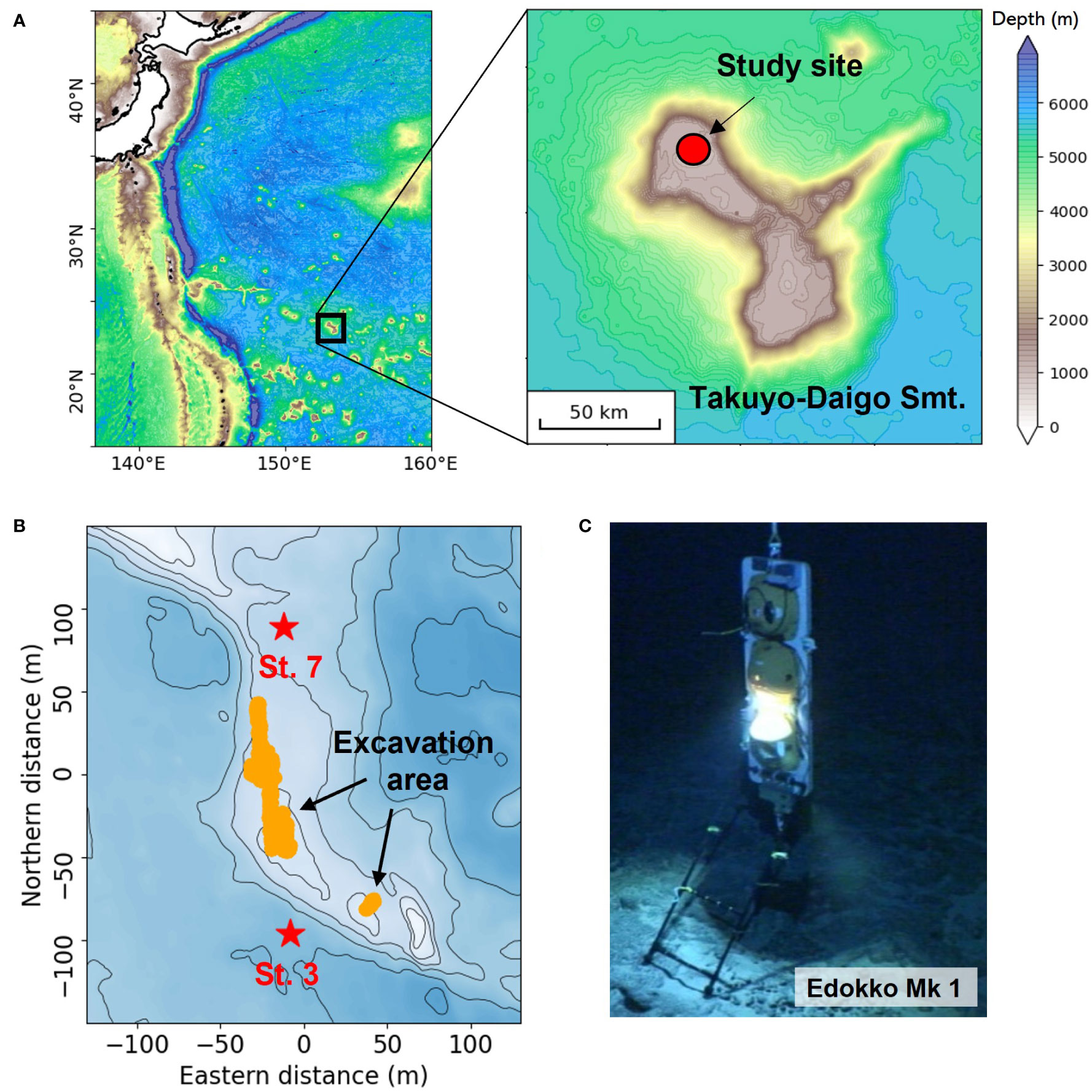
Figure 1 Study site (A, B) and the deep-sea bottom monitoring device “Edokko Mark 1 HSG type” (C). In (B), the red stars represent sites of image collection, the area in orange represents the location of the excavator operation during the excavation test. For bathymetry of the study site which was at ~950 m, contour lines are for every 2 meters with blue being deeper.

Image collection

The deep-sea monitoring device “Edokko Mark 1 HSG type” (Okamoto Glass Co., Ltd.) was installed at two locations in the north and south of the study site (St. 3 and St. 7) to capture video (Figures 1B, C). The two locations were selected close (~50 – 100 m) to the excavation area to allow for comparison between sites and represent different levels of sediment deposition. Based on preliminary flow observations and sediment-plume modelling, the plume from the excavation was expected to flow primarily towards St.3 with relatively little towards St.7 (Suzuki et al, in review). The video recording period was from June 23 to July 30, 2020. The shooting time was set to 1 minute every 4 hours from June 23 to July 2 to extend battery life, and 1 minute every hour from July 3 to July 30 for detailed observation. The 2 seconds between when the lights were turned on until the brightness of the lights stabilized was removed from all videos before analysis. The camera was approximately 1.2 m from the bottom, at an angle of approximately 64° to the bottom, and with a horizontal angle of view of approximately 110° (in air). The screen resolution was 1080 p/30 fps. Illumination was approximately 1.6 m above the bottom, at an angle of approximately 30° to the bottom, and at a half illumination angle of ±60° (in air). The total luminous flux was approximately 4000 lumens (in air). An example of the acquired images is shown in Figure 2. Suspended particles were white or translucent and were around ten pixels in size.

FIGURE 2

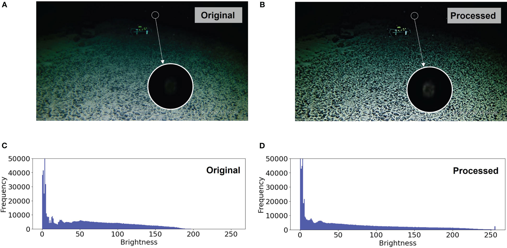
Figure 2 Examples of images at St. 3 which are original (A) and pre-processed with edge-preserving smoothing filter (B). (C, D) are histograms of the HSB color model with pixel brightness (range 0-255) on the horizontal axis, (C) for the original image and (D) for the processed image. The objects in the upper center of the screen are instruments that are not relevant to this study.

Suspended particles detection

Pre-processing of image

When analyzing underwater images, pre-processing is performed to facilitate the identification of objects. In this study, an edge-preserving smoothing filter was used as a processing method to emphasize suspended particles. In water, light absorption by water and scattering of light by suspended particles and plankton cause image degradation such as color distortion, contrast reduction, and blurring. In previous studies, underwater image preprocessing methods by pixel values correction, physical modeling (Ancuti et al., 2018; Dai et al., 2020; Li et al., 2020; Zhang et al., 2022), and deep learning (Islam et al., 2019; Wang Y. et al., 2019; Anwar and Li, 2020; Li et al., 2020; Jian et al., 2022) were proposed. The goal of these methods is to make the target, such as seafloor or organisms, more visible by restoring color and removing haze. However, suspended particles are considered as noise that should be removed, making existing pre-processing methods for underwater images likely counterproductive in this study. The edge-preserving smoothing filter is a process that preserves the contour lines of the object while smoothing the rest of the image as noise. Therefore, it can be useful in both enhancing the contours of suspended particles and removing blurring. Typical examples include median filter and bilateral filter (Tomasi and Manduchi, 1998; Zhu et al., 2019; Chen et al., 2020). In this study, we used the domain transform filter by Gastal and Oliveira (2011), which is based on a transform that defines an isometry between curves on the 2D image manifold in 5D and the real line. This filter is implemented as a “detail enhancement” function in OpenCV (Intel), a Python library for computer vision, for easy and quick processing. Figure 2 shows the original and processed images and their brightness histograms. The filter processing enhanced the light and dark parts of the images and made the particles sharper.

Model training and validation

An object detection algorithm YOLOv5 (Ultralytics, https://github.com/ultralytics/yolov5) was used to create the suspended particle detection model. YOLOv5 is the fifth generation of You Only Look Once (YOLO) (Redmon et al., 2016), released in June 2020. YOLO performs one-stage object detection using convolutional neural networks. YOLOv5 has four training models (s, m, l, x) with different computational load and detection accuracy. In this study, YOLOv5x, which has the highest computational load and detection accuracy, was selected since the particles targeted have few features and are likely difficult to detect. The training and validation data were images captured every 1 second on July 3, 7, 11, 14, and 20 at St. 3. These days were selected because they contained a relatively large number of particles, with the goal of increasing the number and variation of data. The training data consisted of 1028 images containing a total of 3484 particles, and the validation data consisted of 255 images containing a total of 958 particles. The ratio of training data to validation data was distributed approximately 8:2 for both the number of images and the number of classes. St. 7 was not used as training data, only for accuracy verification using the validation data. This allows us to examine whether the detection model works accurately when the location (background of the image) is changed. As with St. 3, the validation data for St. 7 consisted of images captured on July 3, 7, 11, 14, and 20. There was a total of 255 images, containing 575 particles. The hyperparameters were the default settings of YOLOv5. The number of epochs, indicating the number of training iterations, was set to 100, and the batch size was set to 4. The input image size was 1280 × 720 pixels. The loss function was the bounding box regression loss with mean squared error. The loss function is a measure of the magnitude of the discrepancy between the correct value (validation data) and the predicted value (detection result), which is used to optimize the model.

The detection accuracy of the model was evaluated based on intersection over union (IOU), a measure of the overlap of the area of the rectangles of the annotations of the correct and predicted values. Assuming that the validation data are ground truth, the rectangle of the validation data is ${\text{R}}_{\text{v}}$, and the rectangle of the detection results is ${\text{R}}_{\text{d}}$, IOU is defined as follows.

$$IOU= \frac{area(R_d{\cap }^{}{R}_v)}{area(R_d{\cup }^{}{R}_v)}$$

The IOU was compared to the threshold value t. When IOU ≥ t, the detection result was considered correct. In this study, the commonly used value t = 50% was used.

Precision (P), which indicates the percentage of detected rectangles that are correct, and recall (R), which indicates the percentage of detected rectangles that should be detected, are defined as follows.

$$P= \frac{True Positive}{True Positive+False Positive}$$

$$R= \frac{True Positive}{True Positive+False Negative}$$

Then, the average precision (AP), a measure of the model’s detection accuracy, is defined as follows.

$$AP= {\displaystyle \underset{0}{\overset{1}{\int }}P(R)dR}$$

In this study, AP50, which means the threshold for IOUs is 50%, was used. AP50 is one of the most common performance indicators for object detection accuracy (Padilla et al., 2020). In addition, the F1 Score, an index that shows the balance between precision and recall, was used to confirm model’s performance:

$$F1= \frac{2}{P^{-1}+ R^{-1}}$$

For both AP50 and F1 Score, the closer to 100 on the percentage scale, the better the model’s accuracy.

Suspended particles detection

Particle detection was performed on captured images at 5-second intervals for each video. Only the upper 40% of the image was used to assess the temporal changes of the particles. The upper 40% of the viewing area was chosen because this was the portion of the image that did not overlap with the seafloor, and similarities in properties between the seafloor and suspended particles hindered detection. The complexity of the seafloor also appeared to cause some areas of false positives in particle detection at the location not used to train the model (see “Results” chapter for details). The average number of particles for each video (particle numbers counted every 5 seconds averaged over 1 minute) was defined as N40, and was used to evaluate time-series changes. N40 was square-root transformed before statistical analysis (2-way ANOVA and Tukey’s HSD test). To focus on rapid increases in suspended particles (described below), we defined a “turbidity event” as a period when N40 was observed to be more than 10x the pre-excavation average. The time required to detect a single image was about 1.5 seconds when a CPU (Intel Core i9-10850K, 3.6 GHz) was used, which was roughly the same whether there were zero or more than 200 particles.

Excavation test

During image collection, the world’s first small-scale excavation test of crusts was conducted (Japan Oil, Gas and Metals National Corporation, 2020). The test period was July 9-16, 2020, and a total of seven dredging excavations were conducted. The total excavation distance was 129 m, the excavation width was 0.5 m, and the total dredging time was 109 minutes (Figure 1B). The excavation area was located on top of a 5-7 m high hill, surrounded by a seafloor at a depth of ~950 m. The excavator moved along the seafloor with a crawler, excavated the crusts with a cutterhead, and collected the excavated material by a dredge hose to supplement the cyclone tank. For further details please see Suzuki et al. (in review).

Result

Detection accuracy

The highest AP50 in the learning process was 85.8%, which occurred at 96 epochs (Figure 3A; Table 1). Therefore, the model trained up to 96 epochs was used in this study. The loss function trend (Figure 3B) showed that the error decreased as the model was trained, and no overlearning occurred. The values converged after approximately 30 epochs, indicating that the number of training iterations was sufficient. For St. 7, which was not used to train the model, the validation results showed an accuracy of AP50 = 87.9% (Table 1). The F1 Scores were >80% for both St. 3 (82.1%) and St. 7 (86.1%) (Table 1).

FIGURE 3

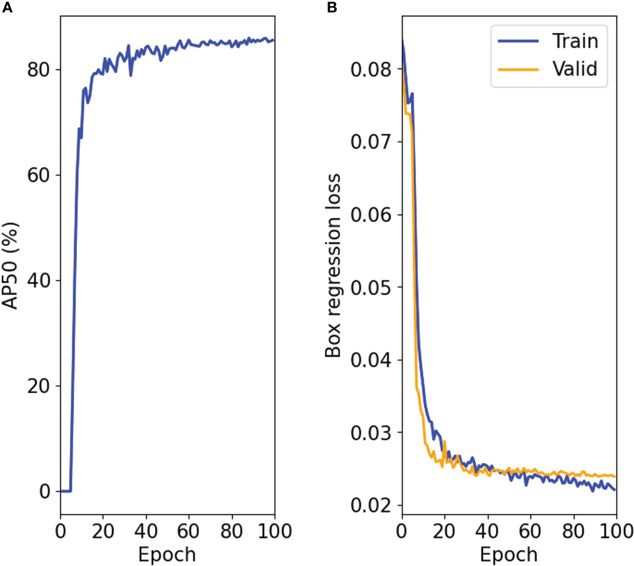
Figure 3 Model training transition. (A) average precision (AP) with 50% thresholds for correct detection, AP50, and (B) box regression loss. The blue line in (B) shows transition of training while the orange line shows transition of validation.

TABLE 1

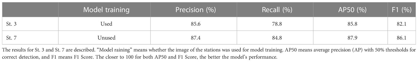
Table 1 Accuracy validation of the detection model.

Examples of model detection results are shown in Figures 4, 5. The sizes of the particles detected ranged from approximately 5 to 20 pixels (Figure S1). Particles were mainly detected in the upper 40% of image where the background was blackish water; in St. 3, the percentage of particles located in the upper 40% was 99%, and in St. 7, it was 97% (Figure 6). On the lower 60% of the image field, where whitish sandy seafloor was the primary background, similar whitish particles were difficult to identify and were rarely detected. Suspended particles that appeared blurred and elliptical due to the fast flow were not detected. The reason for these non-detections was that particles with indistinct contours were not included in the training data in order to avoid false positives for the seafloor and organisms. In the lower part of St. 7, there were two areas of false positives, which corresponded to whitish sediment patches (Figures 6B, C). Other factors that could contribute to false detections include the appearance of organisms such as shrimp and fish, or the slight swaying of the camera system itself due to the current, but manual visual inspection of the images confirmed that these were not an issue with our dataset (Figure S2).

FIGURE 4

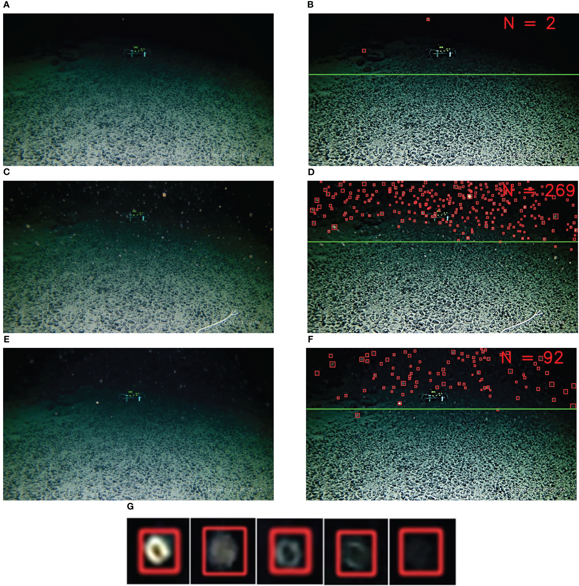
Figure 4 Examples of original images (left column) and particle detection results (right column) in St. 3. Detected particles are surrounded by red rectangles. The number in the upper right corner of the detected image represents the number of particles. The green lines crossing the images show the upper 40%. The images in the right column were pre-processed to enhance light and dark areas. Images were taken at (A, B) 15:00 on July 3 (before excavation test), (C, D) 10:00 on July 11 (turbidity event during excavation test), and (E, F) 16:00 on July 20 (turbidity event after excavation test). (G) examples of detected particles. The objects in the upper center of the screen are instruments that are not relevant to this study.

FIGURE 5

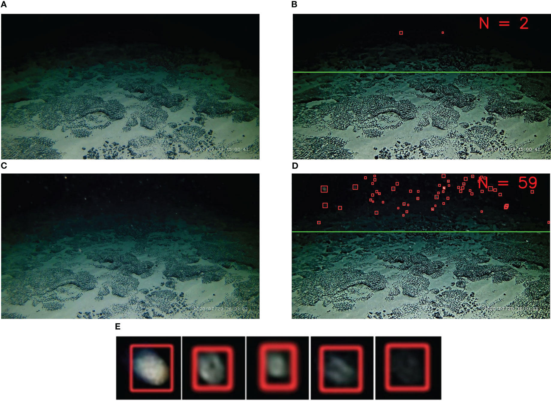
Figure 5 Examples of original images (left column) and suspended particle detection results (right column) at St. 7. Images were taken at (A, B) 15:00 on July 3 (before excavation test) and (C, D) 16:00 on July 20 (turbidity event after excavation test). (E) examples of detected particles.

FIGURE 6

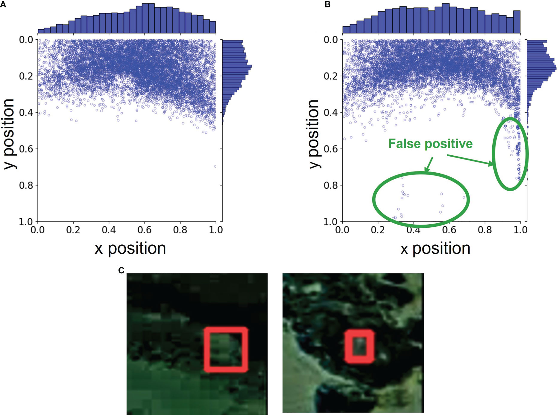
Figure 6 Positions of the detected particles. The vertical and horizontal axes represent the x and y coordinates on the image, normalized from 0 to 1, respectively. (A) St. 3 and (B) St. 7. (C) example of an area of false positives caused by whitish sediment in St. 7.

Fluctuation in suspended particle abundance

The 2-way ANOVA found statistically significant differences for the number of particles detected in the upper 40% of images, N40, between St. 3 and St. 7 (F_{1, 1390 =} 106.44, p< 0.001) and among times (i.e., before, during and after the excavation) (F_{2, 1390 =} 7.51, p< 0.001), while the interaction term for station and time was not significant (F_{2, 1390 =} 0.01, p = 0.988). Spectral analysis including the entire duration of the study revealed no tidal (diurnal or half-diurnal) variation in the time series of N40 (Figure S4).

Natural conditions

Under natural conditions (before the excavation test), N40 had mean values of 3.6 and 2.3 with maximum values of 18.5 and 15.8 for St. 3 and 7, respectively (Table 2, Figure S3). There was a significant difference between St. 3 and St. 7 (Tukey’s HSD test, p< 0.001). Standard deviation was half of the mean for each station before excavation (Table 2).

TABLE 2

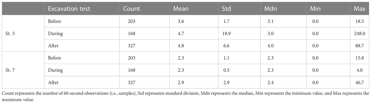
Table 2 The values for the number of particles detected in the upper 40% of images, N40, for the entire observation period divided into before, during, and after the excavation.

Conditions during and after the excavation test

During the excavation test N40 had mean values of 4.7 and 2.3 with maximum values of 248.0 and 4.0 for St. 3 and 7, respectively. After the test, $$N40 had mean values of 4.8 and 2.9 with maximum values of 88.7 and 46.7 for St. 3 and 7, respectively (Table 2, Figure S3). There was a significant difference between St. 3 and St. 7 both during (p< 0.001) and after (p< 0.001) the excavation. During excavation standard deviation was ~4 times the mean for St. 3, but only 22% of the mean for St. 7. After excavation standard deviation was roughly the mean at both stations (Table 2).

At St. 3, there was no significant difference between before, during, and after excavation (p > 0.1); however, at St. 7, the number of particles after excavation was significantly larger than the number of particles both before (p< 0.01) and during (p< 0.01) excavation.

Turbidity events

The N40 showed 3 turbidity events during the observation period, two at St. 3 and one at St. 7, which all occurred either during or after the excavation (Figure 7). For St. 3, the first event was on July 11 at 10:00 during excavation (maximum N40 = 248.0) and was observed at only this time. The second event occurred four days after the end of the excavation test on July 20 and was observed from 13:00 to 20:00 (maximum N40 = 88.7). For St. 7, the turbidity event occurred on July 20 and was observed from 14:00 to 19:00 (maximum N40 = 46.7). For both St. 3 and St. 7, the maximum N40 after the excavation test occurred at 16:00 on July 20 (Figure 7).

FIGURE 7

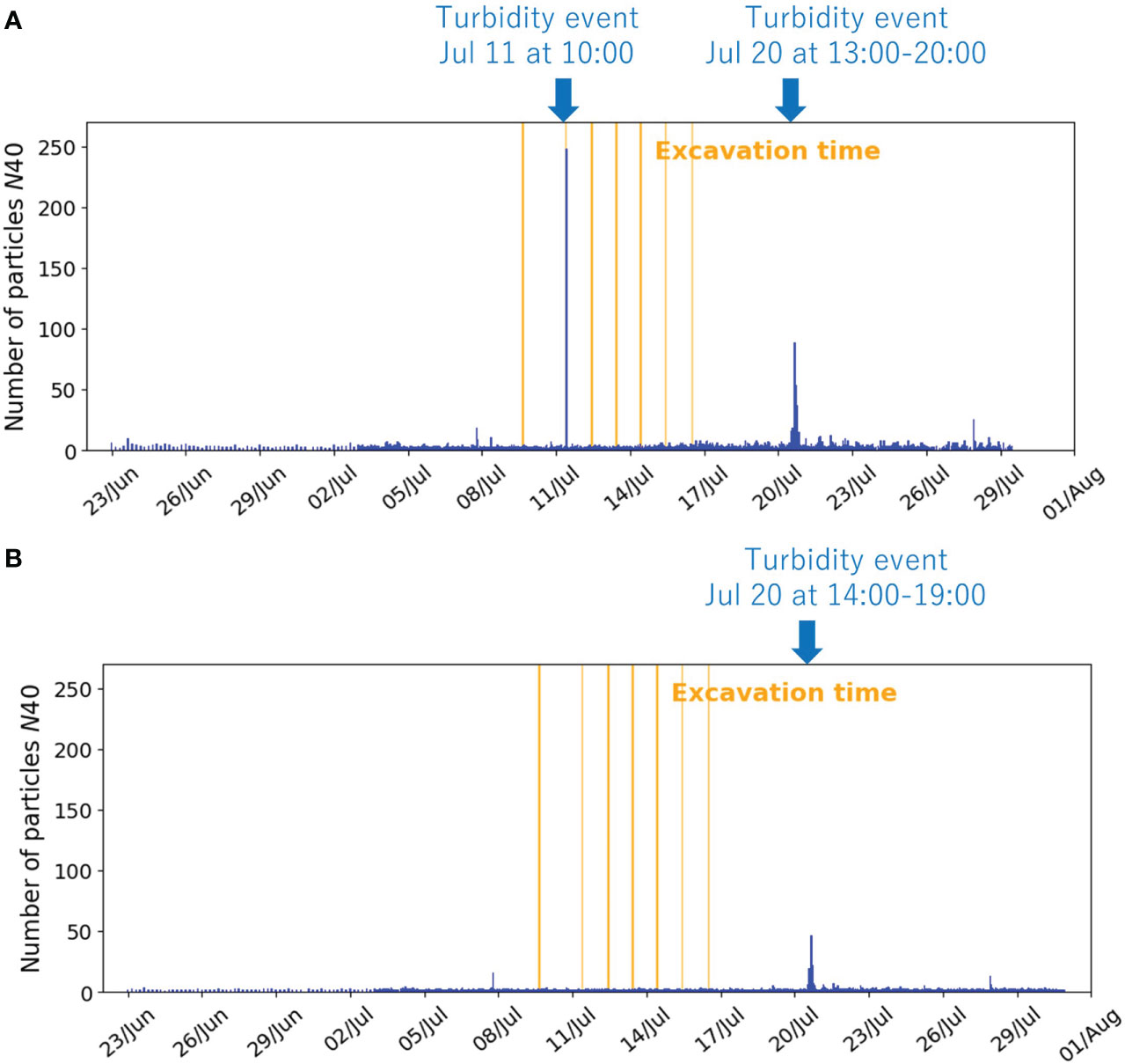
Figure 7 Temporal changes of the number of detected particles in the upper 40% of images, N40 for (A) St. 3 and (B) St. 7. The orange vertical lines indicate the times of excavation.

Discussion

The results of this study suggest that object detection with deep learning may serve as a valuable tool for assessing suspended particle abundance in the deep sea using image datasets. The detection model could detect particles in images with high accuracy at locations used for both model training and those not used (Table 1; Figures 4, 5). The model enabled us to assess temporal changes of particles, including natural small-scale variability and rapid increases possibly caused by anthropogenic disturbance (i.e., small-scale crusts excavation test) (Figure 7).

The detection model’s wide measurement range combined with the ease of eliminating artifacts and possibility of examining both short and long time scales suggest that our method for examining deep-sea suspended particle concentrations can compensate for many shortcomings of existing methods. The detection model was able to measure from zero to hundreds of particles in an image, which may help overcome the detection limits of optical sensors (Gardner et al., 1985; Omar and MatJafri, 2009). To measure low concentrations by optical sensors, it is useful to narrow the measurement range to a higher sensitivity. However, Baeye et al. (2022) measured seafloor disturbance tests with turbidimeters and found that low range turbidimeters are often saturated. Also, measuring low turbidity with optical sensors can often produce electronic noise (Omar and MatJafri, 2009). A detection model that can easily visually identify whether noise is artificial or not (see Figure 6) may be useful as a reference for optical sensors. The fine time scale measurements of the detection model can also complement the sparseness of the measurements generally associated with water sampling. In our study, the measurement interval was 1 – 4 hours, but it can be further fine-tuned according to the interval of image capture. Because detection models can cover a large area, they may be better suited as a monitoring tool than specialized camera systems which generally examine trace amounts of seawater, such as VPR (Davis et al., 2005) or UVP (Picheral et al., 2010). Since one of the objectives of special camera systems is to observe the morphology of plankton and particles, there is a tradeoff between the delicacy of image quality and the narrowness of the measurement space (Lombard et al., 2019). The basic principle of the method in this study is the same as that of the special camera system in the sense that it measures particles in the image. However, the general stationary camera used in this study captured reflected light over a wider area, allowing it to measure sparsely distributed particles, as shown in Figures 4B, 5B. As a bonus, general stationary cameras are much cheaper and user-friendly than specialized camera systems and are commonly used in various deep-sea studies.

Our study is the first that we know of to attempt to use deep learning to quantify suspended particle abundance. While other computational methods exist besides deep learning which may serve useful in quantifying suspended particles, such as binary processing and motion detection, these methods have inherent characteristics that may lead to false measurements. Binary processing, which separates images into background and target objects, may be able to measure particles that stand out against a black background, but if objects other than particles, such as organisms, are captured in the image, they too will be separated from the background and subject to measurement. Motion detection, which detects moving objects against a fixed background, may also be an option for observation of flowing particles (Neri et al., 1998); however, in our study, the video (images) included mobile shrimp and fish while motion was also created by the slight swaying of the camera system itself caused by the current. The use of motion detection would also prevent the use of the vast amounts of video data collected during ROV dives. In general, using deep learning to train a system with target examples is much easier than manually programming the process to predict and avoid all possible false positive targets as described above (Jordan and Mitchell, 2015), greatly reducing the need for manual visual confirmation and additional processing. One remaining challenge is that false positives occurred in certain areas of the seafloor at the station not used for model training (Figure 6), but this can be addressed by increasing the diversity of the dataset used for training (e.g., variations in the environment and shooting conditions).

Our model results suggest that similar evaluations using this method can be made for image data from various locations and also areas where no trained data are used. Most of the particles detected were in the portion of the image where the background was blackish water, and by extracting only the detection results from that part, the possibilities of false positives were greatly reduced. In deep water, where no sunlight reaches, the background is always black water at any location unless the seafloor is captured, and turbidity is generally low, so the environmental conditions affecting the images are fairly similar regardless of specific habitat. Therefore, the model may be similarly accurate for any deep-sea image data set. However, it should be noted that the image dataset used in this study is for only two sites, and could be insufficient in terms of quantity and diversity. It is still necessary to test the model’s performance using data sets with a greater variety of shooting and environmental conditions. Much of the work on underwater object detection has been done on fish (Ditria et al., 2020; Salman et al., 2020; Bonofiglio et al., 2022; Kandimalla et al., 2022; Knausgård et al., 2022), which, although they look and behave differently from suspended particles, could be a useful reference for dataset collection. Ditria et al. (2020), which targeted one type of fish for detection, tested the model’s performance accuracy on images from the same estuarine region as the training data and on images from a different estuarine region, and found similarly high accuracy (> 92% for F1 Score and AP50). Salman et al. (2020), which proposed a method to detect moving fish, demonstrated that the approach is robust to image variability using a large underwater video repository containing diverse environments and fish species (> 80% for F1 Score).

Future work required to improve our particle-detection method includes extending the diversity of image datasets used for accuracy validation and identifying the limits of applicability of the model. Examples of future datasets to explore include images from habitats with a wide range of environmental conditions including particle size, suspended particle concentration, and flow velocity (how fast flowing blurry particles can be detected). In terms of imaging conditions, particular attention may need to be paid to lighting, which affects the visibility of suspended particles (Walther et al., 2004; Cyganek and Gongola, 2018). The detection results also need to be calibrated with physical collections of suspended particles to convert what is essentially qualitative data into actual quantitative data. Otherwise, they cannot be compared with observations from other studies (e.g., Biscaye and Eittreim, 1977; Gardner et al., 2018). Laboratory dilution methods that convert turbidimeter readings (formazin turbidity units, FTU) to concentrations (mg/L) may be a reference for calibration. For example, Spearman et al. (2020) diluted sediment samples with seawater from the field to create suspensions of known concentrations. Optical sensors were then immersed in these suspensions and their FTU readings were recorded, and this process was repeated over a range of concentrations. For future work, a similar calibration may be possible by replacing the optical sensor with a camera and using a water tank. Furthermore, even if abrupt changes due to anthropogenic impacts are measured, it is still remains largely unknown what thresholds of suspended particles will be ecologically relevant (Washburn et al., 2019; Drazen et al., 2020), although this work is not directly related specifically to our methods.

Our model may provide new insights into temporal changes of suspended particles. The extremely low N40 values before the excavation highlight the difficulties of measurement by previous methods. But the fact that these particles constitute the primary food source of organisms in the deep sea (Lal, 1977; Alldredge and Silver, 1988) suggest that changes in observed particles from, for example, N40 = 1 to N40 = 10 would constitute a possible 900% increase in food supply. Thus, even “small” temporal variability may be of large importance in the deep sea, and our detection model may be able detect these miniscule changes.

The observations following the excavation test also have interesting implications on future impacts of deep-sea mining. The cause of differences in average N40 among time periods and the rapid increases of particles, or turbidity events, may be a sediment plume of broken crust particles, a large amount of resuspended sediment generated by disturbance, or resuspension of natural sediment or sediment deposited from the plume after excavation (Sharma et al., 2001; Aleynik et al., 2017). The fact that for N40 at St. 7, there was no difference before and during the excavation test, but there were differences before and after and during and after may suggest that once deposited, the particles from excavation increased the amount of suspended particles in the surrounding area over time due to resuspension (Sharma et al., 2001; Aleynik et al., 2017). However, human disturbance is often associated with increased variability, and the extremely large standard deviation during the excavation at St. 3 compared to other times suggests that there may have been alterations in suspended particle concentrations during the test as well (Table 2). Much remains unexplored about dynamics of sediment plumes (Washburn et al., 2019; Drazen et al., 2020) and resuspension in deep-sea seamounts (Turnewitsch et al., 2013). These likely causes are not discussed in detail because they are beyond the scope of this paper which is focused on methodology. For further details please see Suzuki et al. (in review). If turbidity events were indeed caused by the excavation test, one would expect there to be plumes generated during each of the 7 excavations. A likely reason why only one event was observed during excavation is that the excavation time was too short to be captured by the one-minute-per-hour video recording. Due to the limitations in our dataset, we chose to use the excavation test as an example of high particle concentrations for our model rather than attempt to focus on and define the extent of impacts from excavation itself. This highlights the importance of carefully considering sampling intervals to ensure the ability to examine particular hypotheses.

A notable advantage of our detection model is that it can be adapted to observational data acquired for other purposes, even opening up the possibility of providing new insights from the thousands of hours of data collected in the past. The detection model is likely to be applicable to any deep-sea region and camera system, as long as the entire image does not show the seafloor. Monitoring deep-sea environments with imagery is a common research topic (Bicknell et al., 2016); therefore, there is already an abundance of image data to which the detection model could potentially be applied. A fundamental challenge for ocean observations is to reduce costs (Wang Z. A. et al., 2019). This challenge is particularly acute in deep-sea surveys where access to the field is difficult (Amon et al., 2022). Leveraging existing imaging data may reduce the need for new surveys and the need for familiarization and installation of specialized equipment, and may allow for rapid data collection at a lower cost. Detection models can be a new option to make better use of existing data and improve our understanding of suspended particles in the deep sea.

Data availability statement

The original contributions presented in the study are included in the article/Supplementary Material. Further inquiries can be directed to the corresponding author.

Author contributions

Conceptualization: NS. Methodology: NS and TW. Writing—original draft preparation: NS and TW. Writing—review and check: SY and AS. Image collection: AS. Training and validation of object detection model: NS. Statistical analysis: NS and TW. All authors have read and agreed to the published version of the manuscript. All authors contributed to the article and approved the submitted version.

Acknowledgments

This project was commissioned by the Agency for Natural Resources and Energy in the Japanese Ministry of Economy, Trade and Industry and the Japan Organization for Metals and Energy Security (JOGMEC). The authors express their appreciation to Yoshiaki Igarashi and Jumpei Minatoya (JOGMEC), and Kazumasa Ikeda (Okamoto Glass Co., Ltd.), and others involved in this project. This study was also supported by Research Laboratory on Environmentally-conscious Developments and Technologies (E-code) at AIST.

Conflict of interest

The authors declare that the research was conducted in the absence of any commercial or financial relationships that could be construed as a potential conflict of interest.

Publisher’s note

All claims expressed in this article are solely those of the authors and do not necessarily represent those of their affiliated organizations, or those of the publisher, the editors and the reviewers. Any product that may be evaluated in this article, or claim that may be made by its manufacturer, is not guaranteed or endorsed by the publisher.

Supplementary material

The Supplementary Material for this article can be found online at: https://www.frontiersin.org/articles/10.3389/fmars.2023.1132500/full#supplementary-material

Supplementary Figure 1 | Size of the detected particles. The vertical and horizontal axes indicate the size in pixels along the x- and y-axes, respectively. Note that many points are plotted overlapping each other.

Supplementary Figure 2 | Example of images showing possible false positive targets. Shrimp, fish, and a rope used to secure the camera system were captured. (A, B) are from St. 3 and (C, D) are from St. 7. The number in the upper right corner of the images represents the number of particles detected by the model.

Supplementary Figure 3 | Box-and-whisker plots of suspended particle counts detected in the upper 40% of images (N40). Plotted separately before, during, and after excavation test at St. 3 and St. 7.

Supplementary Figure 4 | Results of spectral analysis on the number of suspended particles detected in the upper 40% of images (N40). (A) St. 3 and (B) St. 7. The data used were taken from July 3, 2020, when the image taking interval was 1 hour.

References

Aleynik D., Inall M. E., Dale A., Vink A. (2017). Impact of remotely generated eddies on plume dispersion at abyssal mining sites in the pacific. Sci. Rep. 7, 16959. doi: 10.1038/s41598-017-16912-2

PubMed Abstract | CrossRef Full Text | Google Scholar

Alldredge A. L., Silver M. W. (1988). Characteristics, dynamics and significance of marine snow. Prog. Oceanogr. 20 (1), 41–82. doi: 10.1016/0079-6611(88)90053-5

CrossRef Full Text | Google Scholar

Amon D. J., Gollner S., Morato T., Smith C. R., Chen C., Christiansen S., et al. (2022). Assessment of scientific gaps related to the effective environmental management of deep-seabed mining. Mar. Policy 138, 105006. doi: 10.1016/j.marpol.2022.105006

CrossRef Full Text | Google Scholar

Ancuti C. O., Ancuti C., De Vleeschouwer C., Bekaert P. (2018). Color balance and fusion for underwater image enhancement. IEEE Trans. Image Process. 27 (1), 379–393. doi: 10.1109/TIP.2017.2759252

PubMed Abstract | CrossRef Full Text | Google Scholar

Anwar S., Li C. (2020). Diving deeper into underwater image enhancement: a survey. Signal Process. Image Commun. 89, 115978. doi: 10.1016/j.image.2020.115978

CrossRef Full Text | Google Scholar

Baeye M., Purkiani K., Stigter H., Gillard B., Fettweis M., Greinert J. (2022). Tidally driven dispersion of a deep-Sea sediment plume originating from seafloor disturbance in the DISCOL area (SE-pacific ocean). Geosci 12 (1), 8. doi: 10.3390/geosciences12010008

CrossRef Full Text | Google Scholar

Bicknell A. W. J., Godley B. J., Sheehan E. V., Votier S. C. V., Witt M. J. (2016). Camera technology for monitoring marine biodiversity and human impact. Front. Ecol. Environ. 14 (8), 424–432. doi: 10.1002/fee.1322

CrossRef Full Text | Google Scholar

Biscaye P. E., Eittreim S. L. (1977). Suspended particulate loads and transports in the nepheloid layer of the abyssal Atlantic ocean. Mar. Geol. 23 (1-2), 155–172. doi: 10.1016/0025-3227(77)90087-1

CrossRef Full Text | Google Scholar

Bonofiglio F., De Leo F. C., Yee C., Chatzievangelou D., Aguzzi J., Marini S. (2022). Machine learning applied to big data from marine cabled observatories: a case study of sablefish monitoring in the NE pacific. Front. Mar. Sci. 9. doi: 10.3389/fmars.2022.842946

CrossRef Full Text | Google Scholar

Brewer P. G., Spencer D. W., Biscaye P. E., Hanley A., Sachs P. L., Smith C. L., et al. (1976). The distribution of particulate matter in the Atlantic ocean. Earth Planet. Sci. Lett. 32 (2), 393–402. doi: 10.1016/0012-821X(76)90080-7

CrossRef Full Text | Google Scholar

Chen B., Tseng Y., Yin J. (2020). Gaussian-Adaptive bilateral filter. IEEE Signal Process. Lett. 27, 1670–1674. doi: 10.1109/LSP.2020.3024990

CrossRef Full Text | Google Scholar

Cyganek B., Gongola K. (2018). Real-time marine snow noise removal from underwater video sequences. J. Electron. Imaging 27 (4), 43002. doi: 10.1117/1.JEI.27.4.043002

CrossRef Full Text | Google Scholar

Dai C., Lin M., Wu X., Wang Z., Guan Z. (2020). Single underwater image restoration by decomposing curves of attenuating color. Opt. Laser Technol. 123, 105947. doi: 10.1016/j.optlastec.2019.105947

CrossRef Full Text | Google Scholar

Davis C. S., Thwaites F. T., Gallager S. M., Hu Q. (2005). A three-axis fast-tow digital video plankton recorder for rapid surveys of plankton taxa and hydrography. Limnol. Oceanogr.: Methods 3 (2), 59–74. doi: 10.4319/lom.2005.3.59

CrossRef Full Text | Google Scholar

Ditria E. M., Lopez-Marcano S., Sievers M., Jinks E. L., Brown C. J., Connolly R. M. (2020). Automating the analysis of fish abundance using object detection: optimizing animal ecology with deep learning. Front. Mar. Sci. 7. doi: 10.3389/fmars.2020.00429

CrossRef Full Text | Google Scholar

Drazen J. C., Smith C. R., Gjerde K. M., Haddock S. H. D., Carter G. S., Choy C. A., et al. (2020). Midwater ecosystems must be considered when evaluating environmental risks of deep-sea mining. PNAS 117 (30), 17455–17460. doi: 10.1073/pnas.2011914117

CrossRef Full Text | Google Scholar

Fulton M., Hong J., Islam M. J., Sattar J. (2019). “Robotic detection of marine litter using deep visual detection models,” in 2019 International Conference on Robotics and Automation (ICRA). (Montreal, QC, Canada: IEEE), 5752–5758. doi: 10.1109/ICRA.2019.8793975

CrossRef Full Text | Google Scholar

Gardner W. D., Biscaye P. E., Zaneveld J. R. V., Richardson M. J. (1985). Calibration and comparison of the LDGO nephelometer and the OSU transmissometer on the Nova scotian rise. Mar. Geol. 66 (1-4), 323–344. doi: 10.1016/0025-3227(85)90037-4

CrossRef Full Text | Google Scholar

Gardner W. D., Richardson M. J., Mishonov A. V., Biscaye P. E. (2018). Global comparison of benthic nepheloid layers based on 52 years of nephelometer and transmissometer measurements. Prog. Oceanogr. 168, 100–111. doi: 10.1016/j.pocean.2018.09.008

CrossRef Full Text | Google Scholar

Gastal E. S. L., Oliveira M. M. (2011). Domain transform for edge-aware image and video processing. ACM Trans. Graph 30 (4). doi: 10.1145/2010324.1964964

CrossRef Full Text | Google Scholar

Glover A., Smith C. (2003). The deep-sea floor ecosystem: current status and prospects of anthropogenic change by the year 2025. Environ. Conserv. 30 (3), 219–241. doi: 10.1017/S0376892903000225

CrossRef Full Text | Google Scholar

Haalboom S., de Stigter H., Duineveld G., van Haren H., Reichart G., Mienis F. (2021). Suspended particulate matter in a submarine canyon (Whittard canyon, bay of Biscay, NE Atlantic ocean): assessment of commonly used instruments to record turbidity. Mar. Geol. 434, 106439. doi: 10.1016/j.margeo.2021.106439

CrossRef Full Text | Google Scholar

Hein J. R. (2004). “Cobalt-rich ferromanganese crusts: global distribution, composition, origin and research activities,” in Minerals other than polymetallic nodules of the international seabed area (Kingston, Jamaica: International Seabed Authority), 188–256.

Google Scholar

Hino H., Usui A. (2022). Regional and fine-scale variability in composition and structure of hydrogenetic ferromanganese crusts: geological characterization of 25 drill cores from the Marcus-wake seamounts. Mar. Georesources Geotechnol. 40 (4), 415–437. doi: 10.1080/1064119X.2021.1904066

CrossRef Full Text | Google Scholar

Islam M. J., Xia Y., Scttar J. (2019). Fast underwater image enhancement for improved visual perception. IEEE Robot. Autom. Lett. 5 (2), 3227–3234. doi: 10.1109/LRA.2020.2974710

CrossRef Full Text | Google Scholar

Japan Oil, Gas and Metals National Corporation (2020) News release: JOGMEC conducts world’s first successful excavation of cobalt-rich seabed in the deep ocean; excavation test seeks to identify best practices to access essential green technology ingredients while minimizing environmental impact. Available at: http://www.jogmec.go.jp/english/news/release/news_01_000033.html (Accessed November 4, 2022).

Google Scholar

Jian Q., Gu Y., Li C., Cong R., Shao F. (2022). Underwater image enhancement quality evaluation: benchmark dataset and objective metric. IEEE Trans. Circuits Syst. Video Technol. 32 (9), 5959–5974. doi: 10.1109/TCSVT.2022.3164918

CrossRef Full Text | Google Scholar

Jordan M. I., Mitchell T. M. (2015). Machine learning: trends, perspectives, and prospects. Science 349 (6245), 255–260. doi: 10.1126/science.aaa8415

CrossRef Full Text | Google Scholar

Kandimalla V., Richard M., Smith F., Quirion J., Torgo L., Whidden C. (2022). Automated detection, classification and counting of fish in fish passages with deep learning. Front. Mar. Sci. 8. doi: 10.3389/fmars.2021.823173

CrossRef Full Text | Google Scholar

Knausgård K. M., Wiklund A., Sørdalen T. K., Halvorsen K. T., Kleiven A. R., Jiao L., et al. (2022). Temperate fish detection and classification: a deep learning based approach. Appl. Intell. 52, 6988–7001. doi: 10.1007/s10489-020-02154-9

CrossRef Full Text | Google Scholar

Lal D. (1977). The oceanic microcosm of particles: suspended particulate matter, about 1 gram in 100 tons of seawater, plays a vital role in ocean chemistry. Science 198 (4321), 997–1009. doi: 10.1126/science.198.4321.997

CrossRef Full Text | Google Scholar

Li A., Anwar S., Porikli F. (2020). Underwater scene prior inspired deep underwater image and video enhancement. Pattern Recognit. 98, 107038. doi: 10.1016/j.patcog.2019.107038

CrossRef Full Text | Google Scholar

Lin T., Goyal P., Girshick R., He K., Dollár P. (2020). Focal loss for dense object detection. IEEE Trans. Pattern Anal. Mach. Intell. 42 (2), 318–327. doi: 10.1109/TPAMI.2018.2858826

CrossRef Full Text | Google Scholar

Liu W., Anguelov D., Erhan D., Szegedy C., Reed S., Fu C.-Y., et al. (2016). “SSD: Single shot MultiBox detector,” in Proceedings ofthe computer vision —ECCV 2016(Cham, Swizerland: Springer), 21–37. doi: 10.1007/978-3-319-46448-0_2

CrossRef Full Text | Google Scholar

Lombard F., Boss E., Waite A. M., Vogt M., Uitz J., Stemmann L., et al. (2019). Globally consistent quantitative observations of planktonic ecosystems. Front. Mar. Sci. 6. doi: 10.3389/fmars.2019.00196

CrossRef Full Text | Google Scholar

Martín J., Puig P., Palanques A., Ribó M. (2014). Trawling-induced daily sediment resuspension in the flank of a Mediterranean submarine canyon. Deep-Sea Res. II 104, 174–183. doi: 10.1016/j.dsr2.2013.05.036

CrossRef Full Text | Google Scholar

Neri A., Colonnese S., Russo G., Talone P. (1998). Automatic moving object and background separation. Signal Process. 66 (2), 219–232. doi: 10.1016/S0165-1684(98)00007-3

CrossRef Full Text | Google Scholar

Omar A. F. B., MatJafri M. Z. B. (2009). Turbidimeter design and analysis: a review on optical fiber sensors for the measurement of water turbidity. Sensors 9, 8311–8335. doi: 10.3390/s91008311

CrossRef Full Text | Google Scholar

Ota Y., Suzumura M., Tsukasaki A., Suzuki A., Seike K., Minatoya J. (2022). Sediment accumulation rates and particle mixing at northwestern pacific seamounts. J. Mar. Syst. 229, 103719. doi: 10.1016/j.jmarsys.2022.103719

CrossRef Full Text | Google Scholar

Padilla R., Netto S. L., Da Silva E. A. B. (2020). “A survey on performance metrics for object-detection algorithms,” in 2020 International Conference on Systems, Signals and Image Processing (IWSSIP). (Niteroi, Rio de Janeiro, Brazil: IEEE), 237–247. doi: 10.1109/IWSSIP48289.2020.9145130

CrossRef Full Text | Google Scholar

Picheral M., Guidi L., Stemmann L., Karl D. M., Iddaoud G., Gorsky G. (2010). The underwater vision profiler 5: an advanced instrument for high spatial resolution studies of particle size spectra and zooplankton. Limnol. Oceanogr.: Methods 8 (9), 462–473. doi: 10.4319/lom.2010.8.462

CrossRef Full Text | Google Scholar

Ramirez-Llodra E., Tyler P. A., Baker M. C., Bergstad O. A., Clark M. R., Escobar E., et al. (2011). Man and the last great wilderness: human impact on the deep Sea. PloS One 6 (8), e22588. doi: 10.1371/journal.pone.0022588

CrossRef Full Text | Google Scholar

Redmon J., Divvala S., Girshick R., Farhadi A. (2016). “You only look once: unified, real-time object detection,” in 2016 IEEE Conference on Computer Vision and Pattern Recognition (CVPR). (Las Vegas, NV, USA: IEEE), 779–788. doi: 10.1109/CVPR.2016.91

CrossRef Full Text | Google Scholar

Salman A., Siddiqui S. A., Shafait F., Mian A., Shortis M. R., Khurshid K., et al. (2020). Automatic fish detection in underwater videos by a deep neural network-based hybrid motion learning system. ICES J. Mar. Sci. 77 (4), 1295–1307. doi: 10.1093/icesjms/fsz025

CrossRef Full Text | Google Scholar

Sharma R., Nagender Nath B., Parthiban G., Jai Sankar S. (2001). Sediment redistribution during simulated benthic disturbance and its implications on deep seabed mining. Deep-Sea Res. II 48 (16), 3363–3380. doi: 10.1016/S0967-0645(01)00046-7

CrossRef Full Text | Google Scholar

Spearman J., Taylor J., Crossouard N., Cooper A., Turnbull M., Manning A., et al. (2020). Measurement and modelling of deep sea sediment plumes and implications for deep sea mining. Sci. Rep. 10, (5075). doi: 10.1038/s41598-020-61837-y

CrossRef Full Text | Google Scholar

Suzuki A., Minatoya J., Fukushima T., Yokooka H., Kudo K., Sugishima H., et al. (in review). Environmental impact assessment for small-scale excavation test of cobalt-rich ferromanganese crusts of a seamount in the northwestern pacific.

Google Scholar

Tan M., Pang R., Le Q. V. (2020). “EfficientDet: scalable and efficient object detection,” in 2020 IEEE/CVF Conference on Computer Vision and Pattern Recognition (CVPR). (Seattle, WA, USA: IEEE), 10778–10787. doi: 10.1109/CVPR42600.2020.01079

CrossRef Full Text | Google Scholar

Tomasi C., Manduchi R. (1998). “Bilateral filtering for gray and color images,” in Sixth International Conference on Computer Vision (IEEE Cat. No.98CH36271). (Bombay, India: IEEE), 839–846. doi: 10.1109/ICCV.1998.710815

CrossRef Full Text | Google Scholar

Turnewitsch R., Falahat S., Nycander J., Dalea A., Scottc R. B., Furnival D. (2013). Deep-sea fluid and sediment dynamics—Influence of hill- to seamount-scale seafloor topography. Earth Sci. Rev. 127, 203–241. doi: 10.1016/j.earscirev.2013.10.005

CrossRef Full Text | Google Scholar

Tyler P. (2003). Disposal in the deep sea: analogue of nature or faux ami? Environ. Conserv. 30 (1), 26–39. doi: 10.1017/S037689290300002X

CrossRef Full Text | Google Scholar

Walther D., Edgington D. R., Koch C. (2004). “Detection and tracking of objects in underwater video,” in Proceedings of the 2004 IEEE Computer Society Conference. (Washington, D.C., USA: IEEE), doi: 10.1109/CVPR.2004.1315079

CrossRef Full Text | Google Scholar

Wang Z. A., Moustahfid H., Mueller A. V., Michel A. P. M., Mowlem M., Glazer B. T., et al. (2019). Advancing observation of ocean biogeochemistry, biology, and ecosystems with cost-effective in situ sensing technologies. Front. Mar. Sci. 6. doi: 10.3389/fmars.2019.00519

CrossRef Full Text | Google Scholar

Wang Y., Song W., Fortino G., Qi L., Zhang W., Liotta A. (2019). An Experimental-based review of image enhancement and image restoration methods for underwater imaging. IEEE Access 7, (99). doi: 10.1109/ACCESS.2019.2932130

CrossRef Full Text | Google Scholar

Wang Y., Yu X., An D., Wei Y. (2021). Underwater image enhancement and marine snow removal for fishery based on integrated dual-channel neural network. Comput. Electron. Agric. 186, 106182. doi: 10.1016/j.compag.2021.106182

CrossRef Full Text | Google Scholar

Washburn T. W., Turner P. J., Durden J. M., Jones D. O. B., Weaver P., Van Dover C. L. (2019). Ecological risk assessment for deep-sea mining. Ocean Coast. Manage. 176 (15), 24–39. doi: 10.1016/j.ocecoaman.2019.04.014"

CrossRef Full Text | Google Scholar

Xue B., Huang B., Wei W., Chen G., Li H., Zhao N., et al. (2021). An efficient deep-Sea debris detection method using deep neural networks. IEEE J. Sel. Top. Appl. Earth Obs. Remote Sens. 14, 12348–12360. doi: 10.1109/JSTARS.2021.3130238

CrossRef Full Text | Google Scholar

Zhang W., Zhuang P., Sun H., Li G., Kwong S., Li C. (2022). Underwater image enhancement via minimal color loss and locally adaptive contrast enhancement. IEEE Trans. Image Process. 31, 3997–4010. doi: 10.1109/TIP.2022.3177129

CrossRef Full Text | Google Scholar

Zhao Z., Zheng P., Xu S., Wu X. (2019). Object detection with deep learning: a review. IEEE Trans. Neural Netw. Learn. Syst. 30 (11), 3212–3232. doi: 10.1109/TNNLS.2018.2876865

CrossRef Full Text | Google Scholar

Zhu F., Liang Z., Jia X., Zhang L., Yu Y. (2019). A benchmark for edge-preserving image smoothing. IEEE Trans. Image Process. 28 (7), 3556–3570. doi: 10.1109/TIP.2019.2908778

CrossRef Full Text | Google Scholar

Zou Z., Chen K., Shi Z., Guo Y., Ye J. (2023). Object detection in 20 years: a survey. Proc. IEEE 111 (3), 257–276. doi: 10.1109/JPROC.2023.3238524

CrossRef Full Text | Google Scholar