A multiple-fluids-mechanics-based model of velocity profiles in currents with submerged vegetation

1 Introduction

Aquatic vegetation is widespread in natural rivers, coasts, and lakes, providing comfortable habitats and abundant food for organisms. This kind of vegetation changes the flow structure and reduces flow velocity and even forms hydraulic jumps because of the vegetation’s resistance, leading to influence on the flow turbulence intensity, sediment, and nutrient transport in flow (Bai et al., 2022; Bai et al., 2022a, b; Shi et al., 1995; Nepf, 1999; Wu et al., 1999; Lou et al., 2022; Yang et al., 2022). Meanwhile, air entrainment takes place when the flow turbulence near the free surface is large enough. A vegetated waterway will promote the flow of energy dissipation and mixing between the water and air, which is of great help in the study of energy dissipation measures (Bai et al., 2022a; Wang et al., 2022). Therefore, it is important to better understand the flow characteristics of vegetated flow and its possible hydraulic impact (Huthoff et al., 2007).

The interaction between submerged vegetation and flow has awakened the broad interest of scholars. The resistance of vegetation to the flow causes a distinct velocity difference between the vegetated layer and upper flow, which causes a strong momentum exchange within the flow in the vegetated layer and the non-vegetated layer alike. This velocity difference is even more obvious especially in the case of large vegetation density. Previous researchers tended to divide the submerged-vegetated flow into several layers and then investigate the flow structure layer-by-layer (Stone and Shen, 2002; Sun and Shiono, 2009). For example, Klopstra et al. (1997) analyzed the vertical distribution of velocity in a flow with flexible submerged vegetation. They applied the Boussinesp concept to describe turbulent shear stresses in the vegetated layer and used the Prandtl mixing length concept in the free surface layer to obtain the logarithmic velocity profile. The velocity in the vegetated layer depends on factors such as slope, water depth, and vegetation characteristics (Yang and Choi, 2010). While in the free surface layer, the viscosity shear stress can also be omitted and only Reynolds shear stress need to be considered (Huai et al., 2009b). Yang et al. (2007) selected plastic grass, duck feathers, and plastic straws to simulate grass, shrubs, and trees, respectively. The distribution of velocity on a floodplain covered by different vegetation was measured. The difference in velocity distribution caused by different aquatic vegetation is mainly reflected in the position of the boundary layer (bottom and top of vegetation). Due to the bed resistance, the velocity near the bottom of the vegetation is low; however, due to the shear stress near the top of the vegetation, the velocity near the vegetation top is greater than that in the inner vegetated layer. The longitudinal velocity in the vegetated layer vertically conformed to an S-type distribution (White and Nepf, 2008; Kowalski and Torrilhon, 2017).

Many models have been proposed to describe the velocity distribution of vegetated flow. Cheng (2015) defined the friction coefficient with a new hydraulic radius and created a single-layer theoretical model for predicting velocity, which was compared with the proposed two-layer model (Stone and Shen, 2002; Baptist et al., 2007; Huthoff et al., 2007; Yang and Choi, 2010; Cheng, 2011). Most two-layer models divide the submerged vegetated flow into a vegetated layer and surface layer by using the top of vegetation as a boundary. The single-layer model was simpler than the two-layer model because it does not involve the calculation of the vegetation drag coefficient and hydrodynamic height of roughness. However, this single-layer model was not suitable for calculating velocity in channels without vegetation and channels with emergent vegetation. Righetti and Armanini (2002) solved the double-averaged (time and space) momentum equations based on the mixing length model and the assumption that turbulent shear stress was quasi-linear, and then they obtained the predicted velocities from the two-layer analytical solution. To explore the hydraulic characteristics of the vegetated and non-vegetated layers, Huai et al. (2009a) used three-dimensional ADV (Acoustic Doppler Velocimetry) to measure the longitudinal velocity with submerged flexible vegetation. They found that the upper part of the vegetated layer was mainly controlled by the K-H vortices while the lower part was mainly controlled by stem vortices caused by the vegetation. In addition, the turbulence intensity and the Reynolds stress reach their maximum near the top of the vegetation. Then, Huai et al. (2009b) proposed a new three-layer model (the inner vegetated layer, the outer vegetated layer, and the upper layer) to predict the vertical distribution of longitudinal velocity in open-channel flow with submerged rigid vegetation. For the upper non-vegetated layer, a modified mixing length theory was adopted. For the inner region near the channel boundary, the mixing length hypothesis is adopted to express the shear stress. And for the outer region within vegetation, shear stress can be simplified by Reynolds stress. The three-layer method can obtain more accurate results of the velocity in the vegetated layer. To obtain a satisfied predicted model of velocity in submerged vegetated flow, Nikora et al. (2013) proposed that the flow was vertically divided into five layers, i.e., the near-bed boundary layer, the uniform velocity layer, the mixing layer at the top of the vegetation, the logarithmic layer above the vegetation, and the wake layer. The near-bed boundary layer could be ignored in most vegetation flows (Nepf and Vivoni, 2000), and the formulas of velocity in other layers were proposed. In the uniform velocity layer, the velocity was related to vegetation resistance and bed slope. The velocity distribution in the mixing layer was complex and can be described by a hyperbolic tangent profile. In the area above the mixing layer, the velocity follows a logarithmic distribution, which should be corrected with the wake term. Shi et al. (2019) thought that the multi-layer method was complex, and people mainly focus on the cross-sectional average velocity of the section, so the traditional two-layer method was used in the flow with submerged rigid vegetation. The force balance equation was adopted in the vegetated layer, and a parameter similar to the Darcy-Weisbach parameter was proposed for the surface layer. This parameter was related to the other parameters through the GP algorithm to obtain a high-precision velocity formula. Different from the traditional layered method, Baruah et al. (2022) proposed a model which was developed by coupling the vegetation drag force with the modified form of two-dimensional shallow water equations. This method can be applied in complex flow scenarios for estimating the vertical distribution of longitudinal velocity in an open channel with submerged, flexible vegetation.

The open-channel flow was used to be divided into two separate layers, namely the submerged vegetation layer and the free surface layer as in the literature (Hui et al., 2009; Ren and Feng, 2020; Zhang et al., 2021). These two layers were mutually independent and the interaction between them was ignored. In the presented article, we consider the complexity of flow structure in the vertical direction and divide the flow into three layers, which are the uniform velocity layer, mixing layer, and logarithmic layer. The mixing layers are formed near the vegetation top. The velocity in the mixing layer is more complex than those in the uniform vegetation layer and logarithmic layer. The purpose of this study is to predict the velocity by applying the superposition principle for the mixing and the logarithmic layers. To obtain the vertical velocity distribution, it is necessary to obtain the velocity additional term in each layer first. The inflection point occurs in the mixing layer according to the literature. The velocity at the inflection point still needs to be discussed. We introduce a corrected parameter β to obtain the predicted velocity at the inflection point and improve the formula for calculating the mixing layer’s width. The model for predicting the velocity profile in the submerged vegetated channel is verified by the measured velocity data from previous studies. The presented paper is organized as follows: Section 2 introduces the methodology, namely the theoretical analysis, followed by a detailed description of model parameters in Section 3. Section 4 introduces the experimental setup and vegetation shape. In Section 5, the predicted and measured velocities are compared. Error analysis, parameter discussion, and model limitations are illustrated in Section 6. A summary of the main findings and conclusions is presented in Section 7.

2 Methodology

In terms of vegetation distribution, the flow structure is divided vertically by the submerged vegetation into two layers: the vegetated layer and the non-vegetated layer, as shown in Figure 1, where the deflected vegetation height is H_v and the water depth is H. The coordinates in the vegetated flow are defined as flow direction x, horizontal direction y, vertical direction z, and the corresponding velocity components are U, V, and W. The vertical distribution of longitudinal velocity is expressed as U_(z), and U_i is the velocity at the inflection point z_i near the vegetation top. Due to the vegetation drag, the velocity difference between the vegetated and non-vegetated layers is distinct, leading to the K-H vortices appearing between the layers. Due to the presence of an inflection point in the velocity profile near the top of the vegetated layer (White and Nepf, 2008), the mixing layer is divided into two layers at the inflection point z_i. δ_o and δ_I are the inner and outer regions of the mixing layer respectively.

FIGURE 1

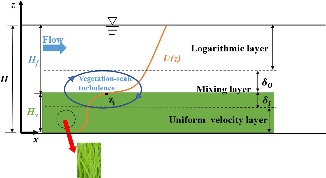
Figure 1 Side view of open channel flow with submerged flexible vegetation.

It is assumed that the velocity can be regarded as a (quasi-) linear superposition of individual mechanisms and the concept of velocity superposition is applied to the whole velocity profile (Nikora et al., 2013). The velocity profile can be divided into three layers. (1) In the uniform velocity layer, i.e., 0< z< z_i - δ_I, U = U_v, where U_v is a velocity in the uniform layer, which is not affected by vortices. (2) In the mixing layer, i.e., z_i - δ_I< z< z_i - δ_o, U = U_v + U_m, where U_m is a velocity additional term in the mixing layer. (3) In the logarithmic layer, i.e., z_i - δ_O< z< H, U = U_v + U_m +U_l + U_w, where U_l is a velocity additional term in the logarithmic layer and U_w is the effect of wake term. The definitions of the specific velocities, i.e., U_v, U_m, U_l, U_w, are elaborated on below.

2.1 Uniform velocity layer

The velocity is set by a balance of vegetation drag and forcing in the inner layer of vegetation (0< z< z_i – δ_I) without effect arising from vortices. The region from 0 to z_i – δ_I in the vertical direction is called the uniform velocity layer. The flow velocity in this layer with the effect of the vegetation drag force can be expressed as (Nepf, 2012):

$\begin{array}{ll}{U}_v={(\frac{gS}{0.5C_{D}a})}^{0.5}& (1)\end{array}$

where g is the acceleration of gravity, S is the bed slope, C_D is the drag coefficient of vegetation, and a is the frontal vegetation area per unit volume. The change of the velocity in this layer mainly depends on the value of C_D and a. Bottom shear is ignored in the uniform velocity layer, and U_v is inversely proportional to the square root of the C_Da. In the case of cylindrical rigid vegetation, C_Da does not change with z in the vertical direction, so U_v remains unchanged. Because of the resistance of vegetation to flow, the velocity in the vegetated layer is always less than the velocity over a bare bed under the same depth and external forcing. According to the principle of momentum balance, Eq. (1) is applicable in both flexible and rigid vegetation.

2.2 Mixing layer

Due to the discontinuity of resistance at the vegetation top, a mixing layer caused by vortices is generated. The distance from the inflection point z_i to the lower boundary of the mixing layer is δ_I, and the distance from z_i to the upper boundary is δ_O (Figure 1). That is, the width of the mixing layer is z_i – δ_I< z< z_i + δ_O. The velocity term U_m is commonly described by a hyperbolic tangent profile (Raupach et al., 1996; Nepf, 2012; Nikora et al., 2013):

$\begin{array}{ll}{U}_m=(U_i-U_v)[1+tanh(\frac{z-z_i}{{\delta }_0})]& (2)\end{array}$

where U_i is the velocity at the inflection point z_i. U_i – U_v = U_s, where U_s is defined as the slip velocity (White and Nepf, 2008). The scale of the vortices gradually develops along the x direction after the flow enters the vegetated layer (Raupach et al., 1996). The flow enters the vegetated layer from the free surface layer in the z direction with the velocity W< 0, indicating the invasion of the vortices. To obtain the U_m, it is necessary to get the velocity U_i at the inflection point first. When the inflection point z_i is at the top of the vegetation, that is, when z_i = $\overline{z}$, the velocity U_i at the inflection point equals the average of the U_v and U₂, i.e., $U_i=(U_v+U_2)/2=\overline{U}$. U₂ is the velocity within the water surface and $\overline{z}$ is the vertical coordinate of $\overline{U}$ (Nikora et al., 2013). However, for a large relative submergence degree, the width of the mixing layer is far less than that of the logarithmic layer, so U_i ≠ (U_v + U₂)/2. The calculation process of U_i is described in detail at the end of the Section 2.

2.3 Logarithmic layer

Significant studies have been carried out on the distribution of turbulent velocity in natural rivers, and the logarithmic velocity distribution formula is widely used (Fu et al., 2013). The logarithmic formula is based on the semi-empirical theory with universality, where parameters are mainly constants and do not depend on the Reynolds number. The velocity distribution above the mixing layer is similar to the open-channel flow, which has a logarithmic shape based on previous experiments (Nepf and Vivoni, 2000; Nepf and Ghisalberti, 2008). The logarithmic term can be expressed as (Nikora et al., 2013), when z_i - δ_O< z< H:

$\begin{array}{ll}{U}_l=\frac{U_{\ast m}}{\kappa }ln\left(\frac{z-d}{z_0}\right)& (3)\end{array}$

$\begin{array}{ll}{z}_0=d{e}^{-\kappa C}& (4)\end{array}$

where U_*m is shear velocity as a momentum transport scale, which is generally equal to the square root of the maximum Reynolds stress; κ (= 0.40) is the Von Kármán constant. The logarithmic formula is appropriate for the open channel flows without vegetation. Owing to the velocity in the vegetated layer not being equal to zero, the calculation starting plane for the logarithmic formula, i.e., a zero plane, should be raised. The zero-displacement height d is approximately equal to the height of submerged vegetation. C = U_i/U_* is the ratio of velocity at the inflected point to the shear velocity. $U_{*}=\sqrt{gHS}$ is defined by Kouwen et al. (1969).

Due to the influence of the side wall and free surface, there is a spiral flow near the water surface that points to the center. The secondary flow brings the low-speed flow near the side wall to the center along the water surface, reducing the surface velocity (Wang et al., 1998). Coles (1956) found that velocity near the water surface deviated from the logarithmic function, and then proposed wake function and wake strength parameter Π to modify the velocity near the water surface. The influence of the wake term on the velocity can be presented using a trigonometric function (Monin and Yaglom, 1971):

$\begin{array}{ll}{U}_w=U_{\ast m}\frac{2\prod }{\kappa }si{n}^2\left(\frac{\pi z}{2H}\right)& (5)\end{array}$

where Π is Coles’s wake strength parameter. For a channel with B/H< 5.20, in which B is the channel width, the maximum velocity point is generally below the flow surface, and for B/H > 5.20, the maximum velocity point is on the flow surface (Fu et al., 2013).

Raupach et al. (1996) stated that the slip velocity U_s = (U₂-U_v)/2. White and Nepf (2008) also obtained the formula of slip velocity: U_s = U_i-U_v through experiments in a channel, which was partially covered by the emergent vegetation. Owing to the different experiment condition, the parameter β is introduced in this paper, i.e., U_i - U_v=β (U₂ - U_v)/2, so that U_i can be obtained iteratively with Eqs. (1) – (5). The verification of the calculated values of U_i and β is discussed in Section 6.2.

3 Parameter determination

The parameters, such as water depth H, vegetated height H_v, the amount of vegetation per unit area m, and the bed slope S can be known easily. To obtain the analytical solution of the velocity distribution, the remaining parameters need to be determined, namely inflection point z_i, velocity U_i at z_i, mixing layer width δ_o + δ_I, frontal vegetation area per unit volume α, drag coefficient C_D, scale of turbulent momentum transport U_*m, and Coles’s wake strength parameter Π.

3.1 Velocity U_i at inflection point z_i

The position of the inflection point z_i in the velocity profile is commonly near the vegetation top. Nikora et al. (2013) showed that the inflection point was slightly lower than the top of the vegetation. In Section 4 illustrating the experimental data, it can be seen that z_i/H_v is taken as 0.75. For cases 4 – 5, z_i/H_v = 0.80. The vegetation density of cases 4 – 5 is smaller than that of cases 1 – 3 (detailed in Section 4), and the scale of vortices is larger in cases 4 – 5. We suspect that this may be a factor influencing the location of the inflection point. U_i is the velocity at the inflection point z_i, which cannot be measured in advance, so U_i - U_v = β(U₂ – U_v)/2 mentioned in Section 2 is solved iteratively to obtain the velocity U_i.

3.2 δ_o and δ_I in mixing layer

White and Nepf (2008) studied the transverse distribution of the velocity in the submerged vegetated channels and gave the width of the mixing layer above the inflection point z_i, which was expressed as:

$\begin{array}{ll}{\delta }_O=\frac{U_2-U_i}{\frac{dU}{dz}{\mid }_{z=z_i}}& (6)\end{array}$

where U₂ is the velocity within the water surface layer.

The width of the mixing layer below the inflection point z_i is the maximum of the drag length scale and the blade width constraint:

$\begin{array}{ll}{\delta }_I=max[0.5{(C_{D}a)}^{-1},1.8D]& (7)\end{array}$

Liu et al. (2013) believed that C_D for the rigid cylindrical vegetation could be taken as 1.00. In cases 1 – 3, based on the mean momentum equation of the vegetated flow for completely developed stage, the effective drag coefficient of the vegetation C_D can be obtained from the study of Huai et al. (2019), which is the relation between measured C_D and z/H_v. In cases 4 – 5, C_D is determined from the experiment of Hui et al. (2009), which is 1.50.

3.3 Model parameter β

The β is introduced in U_i - U_v = β(U₂ - U_v)/2. The value of β is likely to be related to the invasion depth of vortices. In cases 1 – 3, the depth of invasion is smaller, which is about 55%, and β is taken as 0.20. In cases 4 – 5, that is about 65%, and β is considered 0.55.

3.4 Shear velocities U_*m and U_*b

U_*m is a velocity scale of the turbulent momentum transport, which is generally equal to the square root of the maximum Reynolds stress, and U_*b is the wall shear stress. In vegetated flow, the shear stress is not constant due to the effects of gravity and the momentum sink within the vegetation (the effects of secondary currents can also be potentially significant), that is, U_*m ≠ U_*b (Järvelä, 2002; Pokrajac et al., 2006; Nikora et al., 2007). U_*b can be expressed as (Nikora et al., 2001):

$\begin{array}{ll}{U}_{\ast b}=\sqrt{gS(H_f+\alpha H_v)}& (8)\end{array}$

where H_f = H - H_v and α is porosity. Based on Nikora et al. (2013)’s study, U_*b ≈ 1.6U_*m.

3.5 Coles’s wake strength parameter Π

The Coles’s wake strength parameter Π has been extensively studied in the literature. For boundary layers and nonuniform open-channel flows, Π depends on the pressure gradient (Coles, 1956; Kironoto and Graf, 1994). For open-channel flows with vegetation, the value of Π needs to be further investigated considering the influence of turbulence which is caused by the vegetation resistance. Fu et al. (2013) summarized the previous experiments on Π and concluded that it had a range of -0.27 – 0.65. A negative value of Π means that after introducing this parameter in the logarithmic layer, the velocity in this layer is smaller than without consideration of it. In the text for cases 1 – 3: Π = 0.30 – 0.40; cases 4 – 5: Π = 0.10.

4 Experiments

4.1 Experiment I

The experiment was conducted in two glass flumes of the State Key Laboratory of Wuhan University by Huai et al. (2019). The tailgate could be used at the end of channels to adjust the water level. Artificial plastic grass was used to simulate natural vegetation, resembling sedges with staggered arrangements, as shown in Figure 2. The measured points were placed at the mid-perpendicular line of two vegetation rows using Acoustic Doppler Velocimetry (ADV) in the section of x = 4.64 m. One measurement point is measured multiple times to get the average value, which is a dual average velocity in time and space.

FIGURE 2

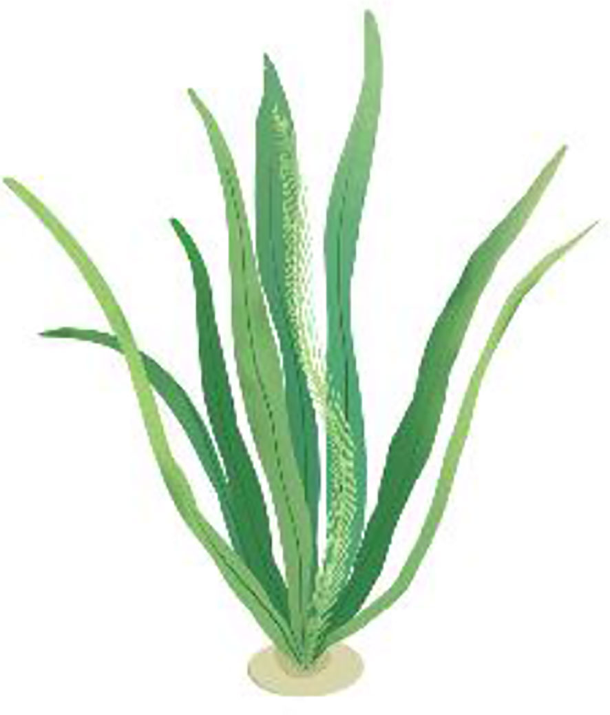
Figure 2 Plastic aquatic grass model.

Referring to the distribution of C_D and a along the vertical direction given by Huai et al. (2019) in the measurement section, the C_Da could be obtained for cases 1 and 2 in Figure 3. It can be seen from Figure 3 that C_Da increased vertically with the increase of z. The model vegetation leaves used in this experiment cause a to reach its peak at the middle of the vegetation and then gradually decrease. The deviation of C_Da from the fitting line near the bed and in the middle of the vegetation increased maybe resulting from the sway of vegetation under the influence of flow.

FIGURE 3

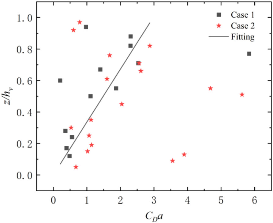
Figure 3 C_Da varies in the vertical direction, where the squares represent case 1, the stars represent case 2, and the straight line indicates the general trend of C_Da along the vertical direction.

4.2 Experiment II

Hui et al. (2009) conducted experiments on shrub-like vegetation in the Hydraulics Laboratory of Tsinghua University to measure the vertical distribution of velocity under various flow conditions. In the experiment, the selected vegetation had an average height of 27.50 cm and an average longitudinal maximum diameter of 20.00 cm. The vegetation was staggered and arranged with two different densities: 15.71/m² and 7.85/m². The velocity distributions in different cross-sections were measured using Acoustic Doppler Velocimetry (ADV). To minimize the influence of spatial heterogeneity on velocity measurement, the velocity at the same depth has been averaged along lateral and longitudinal directions. The ratio of the roots-to-crown diameter was k = 0. 25, that is, the diameter of the vegetation root was 5.00 cm (Figure 4). The drag coefficient of vegetation C_D was 1.50. The corresponding information for the experimental setup is shown in Table 1.

FIGURE 4

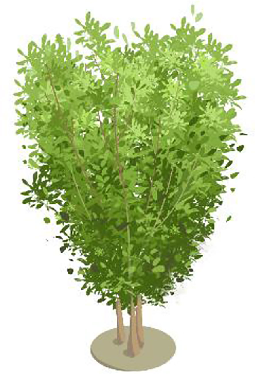
Figure 4 Schematic diagram of a shrub vegetation model.

TABLE 1

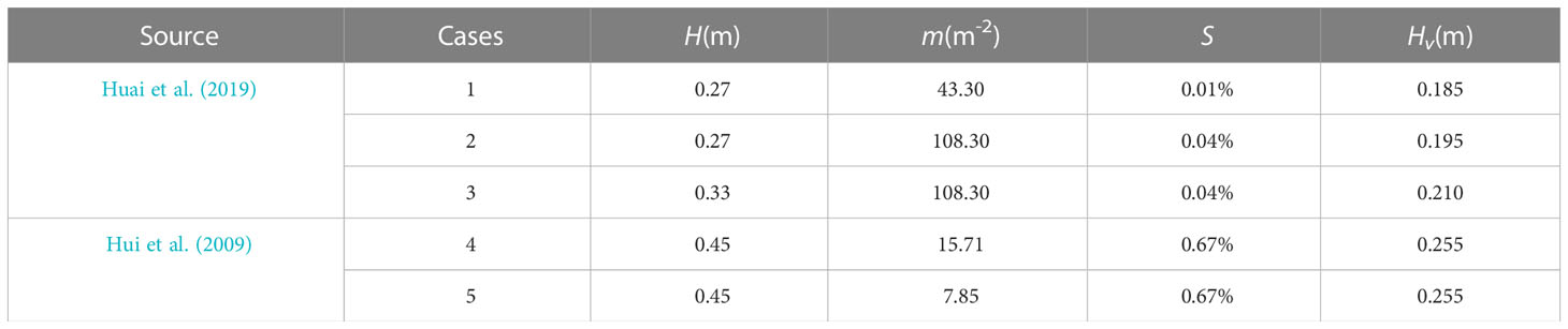
Table 1 Summary of experimental conditions, where H is water depth, m is the amount of vegetation per unit area, S is bed slope, and Hv is deflected vegetation height.

5 Model verification

The comparison between the analytical solution of the proposed model and the measured data along the vertical direction in flow with submerged flexible vegetation is shown in Figure 5. The analytical solution of the velocity distribution in the vertical direction agrees well with the measured data. The area between the two solid black lines is the mixing layer, the area below is the uniform velocity layer, and the area above is the logarithmic layer. The dotted line in the mixing layer represents the vegetation top. In Figure 5, we can see that the velocity in the logarithmic layer (z_i + δ_o< z< H) is much larger than that in the uniform layer (0< z< z_{i -} δ_I) for all subplots. Due to the vertical variance of the vegetation frontal area, the velocity in the vegetated layer (0< z< z_i) showed the “S” shape distinctly in Figures 5A–C. The closest velocity to the channel bed is much smaller than that in the uniform velocity layer, which is due to the friction of the channel bed. Specifically, the velocity near the vegetation bottom is larger than that near the upper of the vegetation in Figure 5, resulting from the C_Da at the top of the vegetation is greater than C_Da near the root. The velocities in the vegetated layer (0< z< z_i) in Figures 5D, E do not show distinct change along the vertical direction due to the relatively uniform value of C_Da. Due to the vortices formed in the mixing layer, the velocity gradient in the region of z_i - δ_I< z< z_i gradually decreases as it approaches the inflection point, followed by a gradual increase of the velocity gradient when z > z_i. The predicted velocity in the logarithmic layer for Figure 5A appears obvious deviations from the measured data, maybe the error of parameter calculation in this case. Overall, the proposed model can be applied in the submerged vegetated channel with different flexibilities and vegetation densities.

FIGURE 5

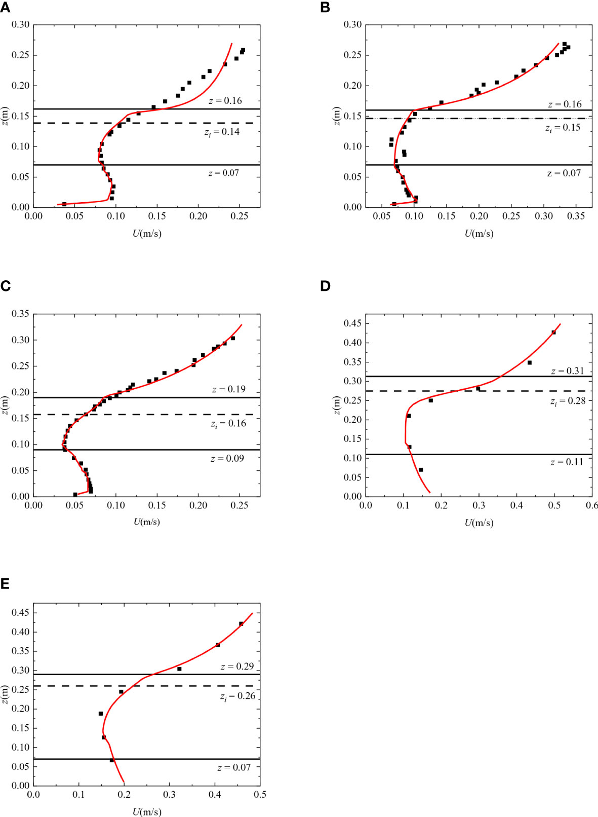
Figure 5 Comparison between the measured velocities and the predicted ones for cases 1 – 5. (A–C) Are the cases from Huai et al. (2019). (D, E) Are the cases of Hui et al. (2019). The solid red lines are predicted data and the points are the measured data. The horizontal dashed lines represent the inflection point, and the region between solid black lines represents the mixing layer.

6 Discussion

6.1 Error analysis

To quantitatively describe the difference between the results of the model and the experimental data, an error analysis from two perspectives: the average values of the absolute error $\overline{ϵ}$ and the relative error $\overline{{ϵ}^{\prime }}$ is performed. The absolute error ϵ is expressed as follows:

$\begin{array}{ll}ϵ=\mid U_{measured}-U_{calculated}\mid & (9)\end{array}$

where the subscripts “measured” and “calculated” represent the measured values and the calculated data from the presented model, respectively. The average value of the absolute error $\overline{ϵ}$ can be expressed as follows:

$\begin{array}{ll}\overline{ϵ}=\frac{1}{N_m}{\displaystyle \sum _{i=1}^{N_m}\mid }{ϵ}_i\mid & (10)\end{array}$

where N_m represents the number of experimental points. The relative error ${ϵ}^{\prime }$ is expressed as follows:

$\begin{array}{ll}{ϵ}^{\prime }=\frac{ϵ}{U_{measured}}& (11)\end{array}$

The average value of the relative error $\overline{{ϵ}^{\prime }}$ is expressed as follows:

$\begin{array}{ll}\overline{{ϵ}^{\text{'}}}=\frac{1}{N_m}{\displaystyle \sum _{i=1}^{N_m}\mid {ϵ}_i\text{'}\mid }\times 100\%& (12)\end{array}$

Table 2 lists the average values of the absolute and relative errors for cases 1 – 5. The average absolute errors of the five cases are less than 0.015 m/s, and the average relative errors of cases 1 – 5 are less than 10%, which reaches the maximum for case 1. The error analysis indicates that the proposed model is reliable in predicting the velocity in the flows with submerged flexible vegetation.

TABLE 2

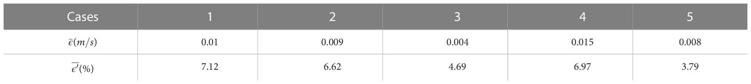
Table 2 Error statistics for measured and predicted velocity.

6.2 Wake strength parameter Π related to U_l

The measured velocities in the logarithmic layer are compared with the predicted data with/without the wake effect for all the cases, which are shown in Figure 6. It can be seen from Figure 6 that the predicted velocity considering the wake effect better agrees well with the measured data than the predicted velocity ignoring the wake effect does. Hence, it is reasonable to conclude that the influence of the wake term on the velocity profile in the logarithmic layer cannot be neglected, which is consistent with the conclusion obtained by Zhang et al. (2021). The Coles’s wake strength parameter Π in the wake function ranges from 0.3 – 0.4 for cases 1 – 3 with the relative submergence H_v/H ≈ 0.7. In cases 4 – 5, Π = 0.1 with the H_v/H = 0.57. The values of Π are all within the range of previous research results (Fu et al., 2013). The relative submergence for cases 1 – 3 is larger than that for cases 4 – 5. We guess that the parameter value of wake strength Π may be inversely correlated with the relative submergence of vegetation. The results show that the Π value has a non-negligible influence on the wake effect, which then influences the velocity profile. Therefore, further experiments for Π are required to refine its application range and to provide better parameter selection for predicting velocity profiles.

FIGURE 6

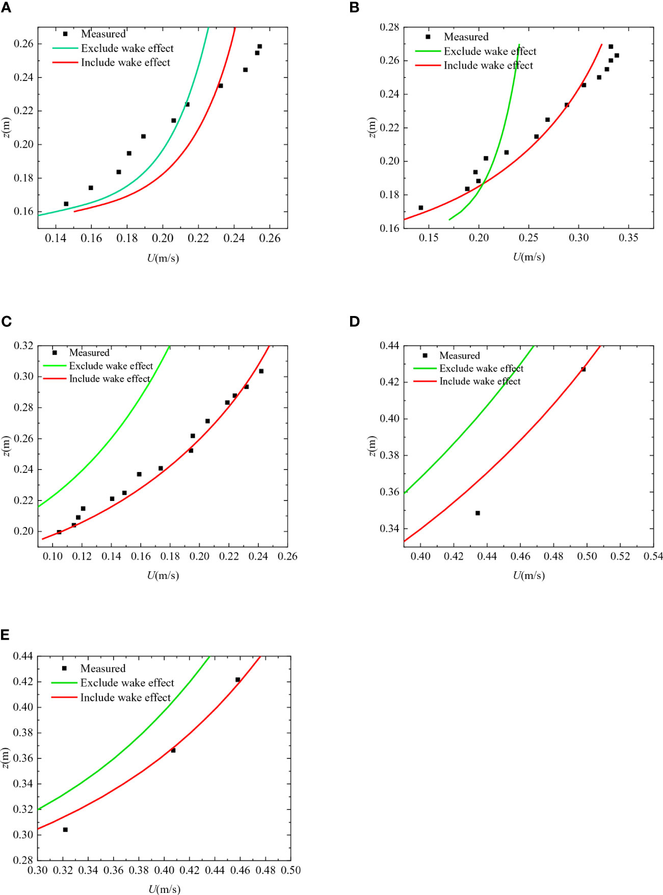
Figure 6 Comparison of the analytical solution and measured values for predicted velocity in the logarithmic layer for cases 1-5. (A–C) Are the cases from Huai et al. (2019). (D, E) Are the cases of Hui et al. (2009). Where the solid green line indicates the model that does not consider the wake effect, and the solid red line indicates that the wake effect is considered.

6.3 Model extension

The proposed model has good application results in flexible vegetated flows, and the following discussion is made to explore its applicability in rigid vegetated flows. We refer to measured data from two different experiments of the rigid vegetated flow. (i) First set of experimental data for rigid vegetated flow was obtained in the Nepf lab at the Massachusetts Institute of Technology (Zhang et al., 2020), where the experimental flume was 24.00 m long and 0.38 m wide, and the water depth H was 0.36 m. The submerged vegetation was constructed from rigid circular rods, the height H_v of which is 0.07 ± 0.002 m, and the diameter was D = 0.64 ± 0.02 cm, where C_D = 1.30, a = 9.60. (ii) Second set of experimental data was conducted by Shi et al. (2023) at the State Key Laboratory of Water Resources and Hydropower Engineering Science. The open channel was partially covered by rigid cylindrical vegetation, the height of which was 0.25 m with a diameter of 8 mm. The water depth was set to 0.35 m. The parameters in the above two cases with rigid vegetation are shown in Table 3.

TABLE 3

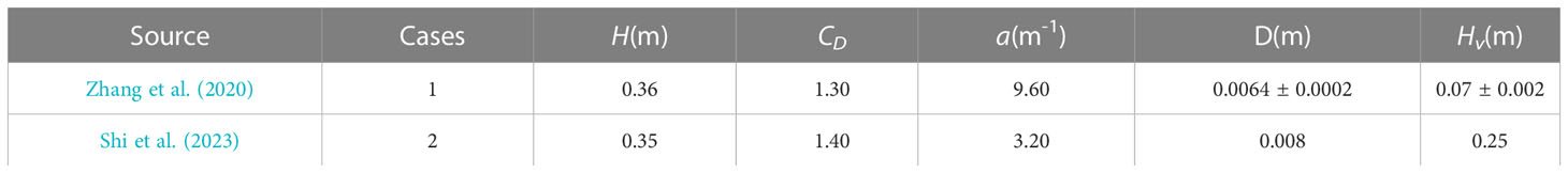
Table 3 Summary of experimental conditions.

A comparison between the predicted and measured data is shown in Figure 7. The measured data is represented by the dots and the predicted data is represented by the blue lines. Although the vegetation densities, vegetation arrangements, and vegetation submergences varied, the predicted velocity from the proposed model could capture the velocity profile in the rigid vegetated flows, showing that this model is also applicable to rigid vegetated flows.

FIGURE 7

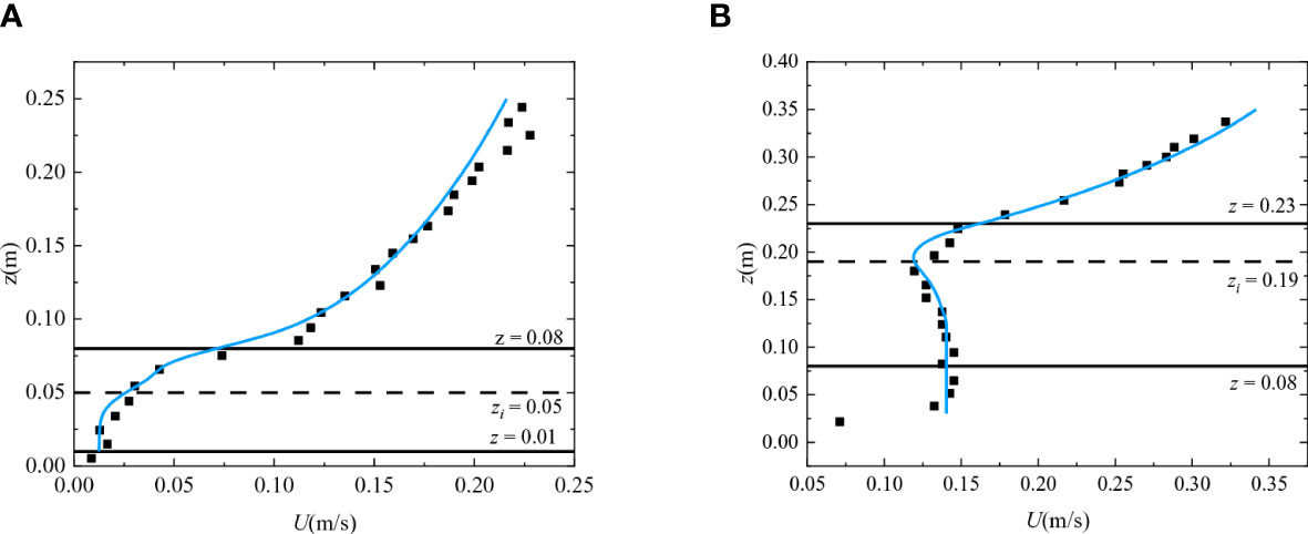
Figure 7 Comparison between the measured and predicted velocities for the rigid vegetation cases, where the solid blue line is the predicted velocity and the points are the measured data. (A) Zhang et al. (2020); (B) Shi et al. (2023). The horizontal lines are the same as those in Figure 5.

6.4 Sensitivity analysis

The influence of β on the prediction of the proposed model is described below. Case 3 is taken as an example. When the target parameter β is adjusted, the other parameters are fixed.

In case 3, the approximate value of β is 0.2 (defined as β₃), and the red solid line in Figure 8 represents the predicted velocity distribution obtained by using β₃. Thus, we considered a wider range of β (= 0.8β₃ – 1.2β₃) to examine the sensitivity of the proposed model. The sensitivity analysis of parameter β is shown in Figure 8. When β< β₃ (e.g., β = 0.8 β₃, the navy blue line), β produces lower velocities in the non-vegetated layer. In contrast, a larger β (e.g., β = 1.1 β₃, the light blue line) corresponds to higher velocities in the non-vegetated layer. According to Figure 8, the predicted velocities are sensitive to the parameter β only in the non-vegetated layer and are insensitive to that in the submerged vegetated layer.

FIGURE 8

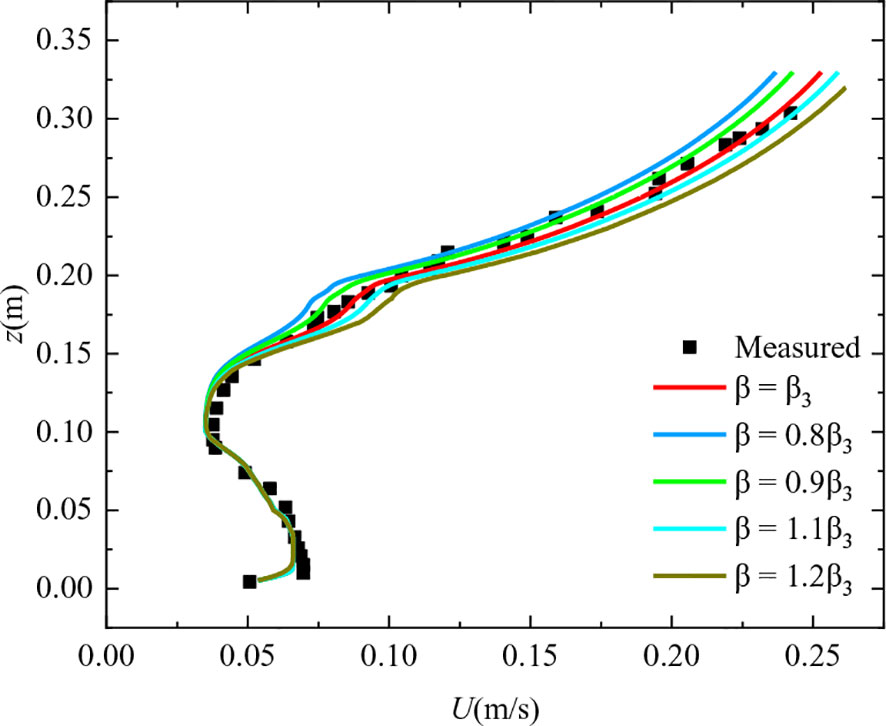
Figure 8 Sensitivity analysis of the parameter β for case 3. β₃ indicates the value of β in case 3. Lines of different colors represent velocity distribution obtained with different β in case 3.

β determines the velocity U_i at the inflection point according to Eq. (2). The velocity U_i at the inflection point z_i of cases 1 – 5 is calculated iteratively. The comparison between the measured and calculated U_i is shown in Table 4, demonstrating that they are basically consistent. The β in cases 1 – 3 is 0.20, which is smaller than 0.55 in cases 4 – 5 with flexible vegetation. It is assumed that the parameter β is related to δ_I, which is the width of the mixing layer below the inflection point z_i. To ensure dimensional homogeneity, the width δ_I is nondimensionalized by the vegetation height H_v. Then, it becomes easy to establish the relationship between the δ and δ_I/H_v, which is $\frac{{\delta }_I}{H_v}=(1.63\pm 0.31) \beta$ for cases 1 – 5 with flexible vegetation and $\frac{{\delta }_I}{H_v}=(4.10\pm 0.30) \beta$ for cases 6 – 7 with rigid vegetation. The averaged velocity $\overline{U}=((U_v+U_2)/2)$ in Table 4. Nikora et al. (2013) noted that $\overline{U}=U_i$ is only applicable to certain cases and has limited application scope. According to Table 4, with the exception of case 1, there are significant differences between the averaged velocity $\overline{U}$ and the measured U_i except case 1. In this study, we introduce a parameter β to obtain the U_i and give explicit expression for β. After introducing β, the calculated U_i agrees well with the measured U_i.

TABLE 4

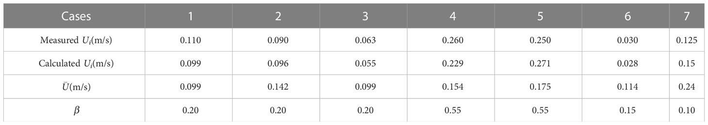
Table 4 Comparison between the calculated and measured velocity U_i.

6.5 Model limitations

It has been proven that the proposed model can be applied to predict the velocity profile in an open channel with submerged flexible/rigid vegetation. The relative submergence of the vegetation and vegetation density leads to the distinct flow structure and then the flow can be vertically divided into separate sublayers. However, for submerged vegetation existing in a river with larger relative submergence and small vegetation density, the width of the uniform layer can be ignored due to the penetration of the mixing layer. For vegetation with smaller relative submergence, the width of the logarithmic layer may decrease and even disappear due to the mixing layer, that is, the mixing layer may be close to the water surface. Given these two above conditions, the flow structure cannot be divided into three layers. More research is needed to explore the influence of relative submergence on the flow structure and velocity profile and then the theoretical model can be improved and applied in more complex cases.

7 Conclusion

The paper presents a model to study the vertical distribution of the velocity in an open channel with submerged flexible vegetation. The model divides the vegetated flow vertically into three layers: uniform velocity layer, mixing layer, and logarithmic layer. In the uniform velocity layer, the influence of vegetation resistance in the prediction of velocity is mainly considered. The vertical distribution of the longitudinal velocity in the mixing layer is similar to the hyperbolic tangent profile, and the conventional logarithmic profile concept is applied in the free surface layer. To obtain the width of the mixing layer divided by the inflection point, a parameter is introduced and iteratively applied to determine the velocity at the inflection point. Due to the influence of momentum transport on the total flow depth, the method of velocity superposition is applied in the mixing layer and logarithmic layer, and then the analytical solution of the longitudinal velocity in the vertical direction can be obtained. According to the error analysis by comparing the predicted velocity with the experimental data, the maximum relative error is 7.12%, indicating that the predicted velocity is reliable. Aquatic vegetation in nature is usually distributed in random patches. Future research can put the focus on the vegetation arrangement, density, and relative submergence to enrich the application range of the presented model, which can be of assistance for ecological understanding such as sediment and pollutant transport.

Data availability statement

The original contributions presented in the study are included in the article/supplementary material. Further inquiries can be directed to the corresponding authors.

Author contributions

All authors made contributions to the conception and design of the study. Material preparation and data collection and analysis were performed by JZ, ZM, HW, WW, ZL, and MG. The first draft of the paper was completed by JZ, ZM, and HW, and all authors commented on previous versions of the manuscript and read and approved the final version.

Funding

The authors declare that this study received funding from the National Natural Science Foundation of China [grant numbers U2040208; 52109100; U2243222], the Joint Open Research Fund Program of State key Laboratory of Hydroscience and Engineering, and Tsinghua – Ningxia Yinchuan Joint Institute of Internet of Waters on Digital Water Governance [grant number sklhse-2023-Iow06], the Postdoctoral Research Foundation of China [grant number 2021M702643], and by Anhui Water Resources Development Co., Ltd. [grant number KY-2021-13]. The funder was not involved in the study design, collection, analysis, interpretation of data, the writing of this article or the decision to submit it for publication.

Conflict of interest

Author MG was employed by Anhui Water Resources Development Co., Ltd.

The remaining authors declare that the research was conducted in the absence of any commercial or financial relationships that could be construed as a potential conflict of interest.

Publisher’s note

All claims expressed in this article are solely those of the authors and do not necessarily represent those of their affiliated organizations, or those of the publisher, the editors and the reviewers. Any product that may be evaluated in this article, or claim that may be made by its manufacturer, is not guaranteed or endorsed by the publisher.

References

Bai R., Bai Z., Wang H., Liu S. (2022a). Air-water mixing in vegetated supercritical flow: effects of vegetation roughness and water temperature on flow self-aeration. Water Resour. Res. 58, e2021WR031692. doi: 10.1029/2021WR031692

CrossRef Full Text | Google Scholar

Bai R., Ning R., Liu S., Wang H. (2022b). Hydraulic jump on a partially vegetated bed. Water Resour. Res. 58, e2022WR032013. doi: 10.1029/2022WR032013

CrossRef Full Text | Google Scholar

Bai G., Xu D., Zou Y., Liu Y., Liu Z., Luo F., et al. (2022). Impact of submerged vegetation, water flow field and season changes on sediment phosphorus distribution in a typical subtropical shallow urban lake: water nutrients state determines its retention and release mechanism. J. Environ. Chem. Eng 10, 107982. doi: 10.1016/j.jece.2022.107982

CrossRef Full Text | Google Scholar

Baptist M. J., Babovic V., Rodríguez Uthurburu J., Keijzer M., Uittenbogaard R. E., Mynett A., et al. (2007). On inducing equations for vegetation resistance. J. Hydraul Res. 45, 435–450. doi: 10.1080/00221686.2007.9521778

CrossRef Full Text | Google Scholar

Baruah A., Sarma A. K., Hinge G. (2022). A semicoupled shallow-water model for vertical velocity distribution in an open channel with submerged flexible vegetation. J. Irrig Drain Eng 148, 06022005. doi: 10.1061/(ASCE)IR.1943-4774.0001704

CrossRef Full Text | Google Scholar

Cheng N. (2011). Representative roughness height of submerged vegetation. Water Resour. Res. 47, W08517. doi: 10.1029/2011WR010590

CrossRef Full Text | Google Scholar

Cheng N. (2015). Single-layer model for average flow velocity with submerged rigid cylinders. J. Hydraul Eng 141, 06015012. doi: 10.1061/(ASCE)HY.1943-7900.0001037

CrossRef Full Text | Google Scholar

Coles D. (1956). The law of the wake in the turbulent boundary layer. J. Fluid Mech. 1, 191–226. doi: 10.1017/S0022112056000135

CrossRef Full Text | Google Scholar

Fu H., Yang K. L., Wang T., Guo X. (2013). Analysis of parameter sensitivity and value for logarithmic velocity distribution formula. J. Hydraul Eng 44, 489–494. doi: 10.13243/j.cnki.slxb.2013.04.014

CrossRef Full Text | Google Scholar

Huai W., Han J., Zeng Y., An X., Qian Z. (2009a). Velocity distribution of flow with submerged flexible vegetations based on mixing-length approach. Appl. Math Mech-Engl 30, 343–351. doi: 10.1007/s10483-009-0308-1

CrossRef Full Text | Google Scholar

Huai W., Zeng Y., Xu Z., Yang Z. (2009b). Three-layer model for vertical velocity distribution in open channel flow with submerged rigid vegetation. Adv. Water Resour. 32, 487–492. doi: 10.1016/j.advwatres.2008.11.014

CrossRef Full Text | Google Scholar

Huai W., Zhang J., Katul G. G., Cheng Y., Tang X., Wang W. (2019). The structure of turbulent flow through submerged flexible vegetation. J. Hydrol 31, 274–292. doi: 10.1007/S42241-019-0023-3

CrossRef Full Text | Google Scholar

Hui E., Jiang C., Pan Y. (2009). Vertical velocity distribution of longitudinal flow in a vegetated channel. j. tsinghua univ. Sci. Technol. 49, 834–837. doi: 10.16511/j.cnki.qhdxxb.2009.06.017

CrossRef Full Text | Google Scholar

Huthoff F., Augustijn D. C. M., Hulscher S. J. M. H. (2007). Analytical solution of the depth-averaged flow velocity in case of submerged rigid cylindrical vegetation. Water Resour. Res. 43, W06413. doi: 10.1029/2006WR005625

CrossRef Full Text | Google Scholar

Järvelä J. (2002). Flow resistance of flexible and stiff vegetation: a flume study with natural plants. J. Hydrol 269, 44–54. doi: 10.1016/S0022-1694(02)00193-2

CrossRef Full Text | Google Scholar

Kironoto B., Graf W. H. (1994). "Turbulence characteristics in rough uniform open-channel flow," in Proceedings of the Institution of Civil Engineers - Water Maritime and Energy 112(4), 336-348. doi: 10.1680/iwtme.1995.28114

CrossRef Full Text | Google Scholar

Klopstra D., Barneveld H., Noortwijk J., Velzen E. (1997). Analytical model for hydraulic roughness of submerged vegetation, American Society of Civil Engineers (ASCE), New-York. 775-780.

Google Scholar

Kouwen N., Unny T. E., Hill H. M. (1969). Flow retardance in vegetated channels. J. Irrig Drain Div. 95, 329–342. doi: 10.1061/JRCEA4.0000652

CrossRef Full Text | Google Scholar

Kowalski J., Torrilhon M. (2017). Moment approximations and model cascades for shallow flow. Commun. Comput. Phys. 25, 669–702. doi: 10.4208/cicp.OA-2017-0263

CrossRef Full Text | Google Scholar

Liu C., Luo X., Liu X., Yang K. (2013). Modeling depth-averaged velocity and bed shear stress in compound channels with emergent and submerged vegetation. Adv. Water Resour. 60, 148–159. doi: 10.1016/j.advwatres.2013.08.002

CrossRef Full Text | Google Scholar

Lou S., Chen M., Ma G., Liu S., Wang H. (2022). Sediment suspension affected by submerged rigid vegetation under waves, currents and combined wave–current flows. Coast. Eng 173, 104082. doi: 10.1016/j.coastaleng.2022.104082

CrossRef Full Text | Google Scholar

Monin A. S., Yaglom A. M. (1971). Statistical fluid mechanics: Mechanics of turbulence, Vol. 1, MIT Press, Boston.

Google Scholar

Nepf H. M. (1999). Drag, turbulence, and diffusion in flow through emergent vegetation. Water Resour. Res. 35, 479–489. doi: 10.1029/1998WR900069

CrossRef Full Text | Google Scholar

Nepf H. M. (2012). Hydrodynamics of vegetated channels. J. Hydraul Res. 50, 262–279. doi: 10.1080/00221686.2012.696559

CrossRef Full Text | Google Scholar

Nepf H., Ghisalberti M. (2008). Flow and transport in channels with submerged vegetation. Acta Geophysica 56, 753–777. doi: 10.2478/s11600-008-0017-y

CrossRef Full Text | Google Scholar

Nepf H. M., Vivoni E. R. (2000). Flow structure in depth-limited, vegetated flow. J. Geophys. Res. 105, 28547–28557. doi: 10.1029/2000JC900145

CrossRef Full Text | Google Scholar

Nikora V., Goring D., McEwan I., Griffiths G. (2001). Spatially averaged open-channel flow over rough bed. J. Hydraul Eng 127, 123–133. doi: 10.1061/(ASCE)0733-9429(2001)127:2(123

CrossRef Full Text | Google Scholar

Nikora V., McLean S., Coleman S., Pokrajac D., McEwan I., Campbell L., et al. (2007). Double-averaging concept for rough-bed open-channel and overland flows: applications. J. Hydraul Eng. 133, 884–895. doi: 10.1061/(ASCE)0733-9429(2007)133:8(884

CrossRef Full Text | Google Scholar

Nikora N., Nikora V., O’Donoghue T. (2013). Velocity profiles in vegetated open-channel flows: combined effects of multiple mechanisms. J. Hydraul Eng 139, 1021–1032. doi: 10.1061/(ASCE)HY.1943-7900.0000779

CrossRef Full Text | Google Scholar

Pokrajac D., Finnigan J. J., Manes C., McEwan I., Nikora V. (2006). “On the definition of the shear velocity in rough bed open channel flows,” in River Flow 2006 (ed. by R. M. L. Ferreira, E. C. T. L. Alves, J. G. A. B. Leal and A. H. Cardoso), 89–98. Taylor & Francis Group, London, UK.

Google Scholar

Raupach M., Finnigan J., Brunet Y. (1996). Coherent eddies and turbulence in vegetation canopies: the mixing-layer analogy. Boundary Layer Meteorol. 78, 351–382. doi: 10.1007/978-94-017-0944-6_15

CrossRef Full Text | Google Scholar

Ren S., Feng M. (2020). Experimental study on hydraulic characteristics of open channel with flexible vegetation. J. Water Resour. Water Eng. 31, 186–192.

Google Scholar

Righetti M., Armanini A. (2002). Flow resistance in open channel flows with sparsely distributed bushes. J. Hydrol 269, 55–64. doi: 10.1016/S0022-1694(02)00194-4

CrossRef Full Text | Google Scholar

Shi H., Liang X., Huai W., Wang Y. (2019). Predicting the bulk average velocity of open-channel flow with submerged rigid vegetation. J. Hydrol 572, 213–225. doi: 10.1016/j.jhydrol.2019.02.045

CrossRef Full Text | Google Scholar

Shi Z., Pethick J. S., Pye K. (1995). Flow structure in and above the various heights of a saltmarsh canopy: a laboratory flume study. J. Coast. Res. 11, 1204–1209.

Google Scholar

Shi H., Zhang J., Huai W. (2023). Experimental study on velocity distributions, secondary currents, and coherent structures in open channel flow with submerged riparian vegetation. Adv. Water Res 173, 104406. doi: 10.1016/j.advwatres.2023.104406

CrossRef Full Text | Google Scholar

Stone B. M., Shen H. (2002). Hydraulic resistance of flow in channels with cylindrical roughness. J. Hydraul Eng 128, 500–506. doi: 10.1061/(ASCE)0733-9429(2002)128:5(500

CrossRef Full Text | Google Scholar

Sun X., Shiono K. (2009). Flow resistance of one-line emergent vegetation along the floodplain edge of a compound open channel. Adv. Water Resour. 32, 430–438. doi: 10.1016/j.advwatres.2008.12.004

CrossRef Full Text | Google Scholar

Wang H., Bai Z., Bai R., Liu S. (2022). Self-aeration of supercritical water flow rushing down artificial vegetated stepped chutes. Water Resour. Res. 58, e2021WR031719. doi: 10.1029/2021WR031719

CrossRef Full Text | Google Scholar

Wang D., Wang X., Li D. (1998). Comparison of the distribution formula of mean flow velocity in open channel and analysis of influencing factors. (in Chinese) J. Sediment Res., 3, 88–92. doi: 10.16239/j.cnki.0468-155x.1998.03.015

CrossRef Full Text | Google Scholar

White B. L., Nepf H. M. (2008). A vortex-based model of velocity and shear stress in a partially vegetated shallow channel. Water Resour. Res. 44, W01412. doi: 10.1029/2006WR005651

CrossRef Full Text | Google Scholar

Wu F., Shen H. W., Chou Y. (1999). Variation of roughness coefficients for unsubmerged and submerged vegetation. J. Hydraul Eng 125, 934–942. doi: 10.1061/(ASCE)0733-9429(1999)125:9(934

CrossRef Full Text | Google Scholar

Yang K., Cao S., Knight D. W. (2007). Flow patterns in compound channels with vegetated floodplains. J. Hydraul Eng 133, 148–159. doi: 10.1061/(ASCE)0733-9429(2007)133:2(148

CrossRef Full Text | Google Scholar

Yang W., Choi S. U. (2010). A two-layer approach for depth-limited open-channel flows with submerged vegetation. J. Hydraul Res. 48, 466 –475. doi: 10.1080/00221686.2010.491649

CrossRef Full Text | Google Scholar

Yang Z., Guo M., Li D. (2022). Theoretical model of suspended sediment transport capacity in submerged vegetation flow. J. Hydrol 609, 127761. doi: 10.1016/j.jhydrol.2022.127761

CrossRef Full Text | Google Scholar

Zhang J., Lei J., Huai W., Nepf H. (2020). Turbulence and particle deposition under steady flow along a submerged seagrass meadow. J. Geophysical Res: Oceans 125, e2019JC015985. doi: 10.1029/2019JC015985

CrossRef Full Text | Google Scholar

Zhang J., Wang W., Shi H., Wang W., Li Z., Tang X., et al. (2021). An analytical two-layer model for velocity distribution in open-channel flows with submerged flexible canopies considering multiply fluids mechanics. J. Hydrol 603, 127102. doi: 10.1016/j.jhydrol.2021.127102

CrossRef Full Text | Google Scholar