Reconstructing three-dimensional salinity field of the South China Sea from satellite observations

1 Introduction

Ocean salinity is essential for the study of global hydrological cycle and ocean circulation, and its variation plays an important role in the ocean stratification, climate change and ecosystem (Lagerloef, 2002; Held and Soden, 2006; Schmitt, 2008; Ren and Riser, 2010; Schmidtko et al., 2017). However, changes in salinity within the ocean, especially within the marginal seas, have not been well captured and understood yet due to the lack of sufficient high-resolution three-dimensional (3D) data. In situ measurements from underwater moorings or profiling floats such as the global array for real-time geostrophic oceanography (Argo) are traditionally used for studying the salinity characteristics of the interior ocean. However, field observations are still sparse, discontinuous, and limited in coverage, which obscure the details of mesoscale and smaller-scale processes. Satellite remote sensing has provided long-term and high-resolution data of various sea surface variables worldwide. However, the sensors cannot directly see the deep ocean where the thermohaline structure shows significant variations due to complex dynamic processes such as mesoscale eddies and internal waves (Henning and Vallis, 2004; Huang et al., 2016; Keppler et al., 2018). By retrieving the 3D salinity field from a large set of satellite data (Klemas and Yan, 2014), it is possible to improve the skill of surface observations to deeper layers and thus better understand marine phenomena at different spatiotemporal scales.

Several methods have been applied to estimate salinity profiles from satellite observations. Before the operational application of salinity satellites such as Aquarius, Soil Moisture and Ocean Salinity (SMOS) and Soil Moisture Active and Passive (SMAP) missions, sea surface salinity (SSS) data were very sparse and very rarely used as model inputs (Carnes et al., 1994; Agarwal et al., 2007; Guinehut et al., 2012). For example, Guinehut et al. (2012) tried to estimate the 3D salinity anomaly field of the global ocean by establishing a linear relationship between monthly Argo salinity profiles on a 1° grid and 7-d sea level anomaly (SLA) with spatial resolution of 1/3°. They concluded that altimeter observed SLA could only reconstruct approximately 20% to 30% of the salinity signal, implying that it is necessary to consider more surface variables for accurate estimation of the vertical structure of salinity. Some studies used field observations of SSS to estimate underwater salinity and found that SSS was an essential parameter for 3D salinity reconstruction (Agarwal et al., 2007; Ballabrera-Poy et al., 2009). Yang et al. (2015) used linear regression and neural network models to retrieve vertical salinity profiles from SSS observed by SMOS. The nonlinear neural network provided more accurate estimation than the linear model in the upper 2000 m of the global ocean, and the root mean square error (RMSE) varies from 0.077 psu to 0.138 psu in different regions. This highlights the potential of artificial intelligence (AI) approach in underwater salinity reconstruction. However, due to the relatively short period of SMOS data at that time, the accuracy was not high enough.

The amount of satellite data has explosively increased in recent years, and as a result, oceanographic research has entered the “big data era” (Li et al., 2020). The combination of ocean big data and AI provides a new way of reconstructing 3D salinity fields from surface variables observed by satellites. Recently, Su et al. (2019) introduced a machine learning method called extreme gradient boosting to estimate global ocean subsurface salinity structure from the anomaly of several surface variables including SSS, sea surface temperature (SST), sea surface height and sea surface wind (SSW). The model uses monthly Argo salinity profiles on a 1° grid as label data, with resultant average normalized RMSE and correlation coefficient of 0.042 and 0.735, respectively. Other machine learning and deep learning methods have also been proposed to obtain the salinity or salinity anomaly profiles in the open ocean from satellite observations, such as the generalized regression neural network (Bao et al., 2019), long- and short-term memory (LSTM) (Buongiorno Nardelli, 2020), convolutional neural network (CNN) (Meng et al., 2022) and convolutional LSTM (Song et al., 2022). Generally, the surface variables used as model inputs include SSS/SSS anomaly, SST/SST anomaly, SLA, SSW/SSW anomaly, or absolute dynamic topography (ADT). However, less attention is given to the reconstruction of interior salinity structure in marginal seas, where it is more difficult to obtain accurate results due to complex topography and multi-scale dynamics. The South China Sea (SCS, Figure 1A) is one of the largest marginal seas adjacent to the West Pacific Ocean, where mesoscale and sub-mesoscale processes are very active (Wang et al., 2003; Zheng et al., 2007; He et al., 2018; Xie et al., 2022a). High-resolution 3D ocean observations are urgently needed to capture the fine structure and evolution of these dynamic processes. Therefore, the reconstruction of 3D salinity fields at high temporal and spatial resolution is necessary for the SCS. To achieve this goal, a U-net deep learning model combined with an attention mechanism (hereafter called “Attention U-net”) is here presented to reconstruct the 3D salinity field in the upper 1000 m of the SCS from satellite observations of SSS, SST, SLA and SSW. The daily vertical salinity profiles on a 1/4° grid from the GLORYS2V4 reanalysis product were used for training and evaluating the network. The paper is organized as follows. Section 2 presents the satellite-observed sea surface variables and reanalysis data of ocean salinity profiles used here. The detailed configuration of the Attention U-net model is also described. The model performance in reconstructing 3D salinity field of the SCS is evaluated in Section 3. In Section 4, the estimation errors are analyzed, and the influence of SSS on the upper-layer salinity reconstruction is discussed. An applicative example of the reconstruction model in revealing the underwater salinity signals related to the mesoscale cold eddy is also shown. Finally, conclusions are given in Section 5.

FIGURE 1

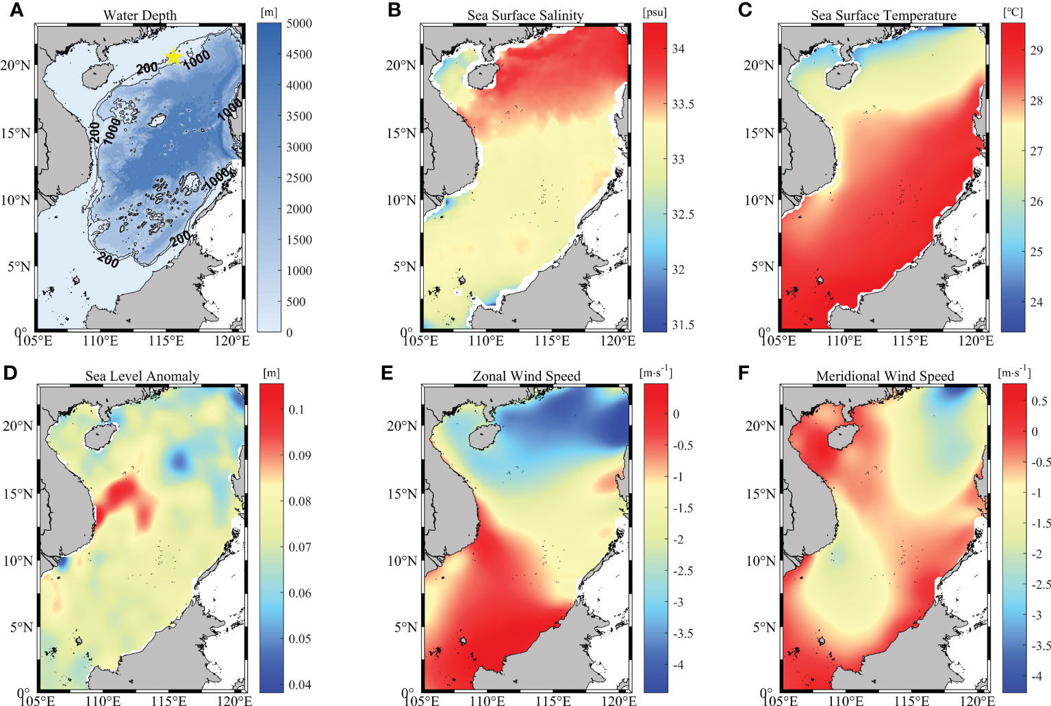
Figure 1 (A) Distribution of water depth in the SCS. Contours of 200 m and 1000 m depth are overlaid with black lines, and the location of a mooring station is marked as a yellow pentagram. (B–F) Climatology of sea surface variables in the SCS from 2010 to 2018. (B) Sea surface salinity, (C) sea surface temperature, (D) sea level anomaly, (E) zonal and (F) meridional wind speed.

2 Materials and methods

2.1 Satellite observations and reanalysis product

The surface variables used as inputs to the Attention U-net model are SSS, SST, SLA, and zonal and meridional components of SSW. The SSS data are provided by the European Space Agency (ESA) Sea Surface Salinity Climate Change Initiative (CCI) consortium (https://data.ceda.ac.uk/neodc/esacci/sea_surface_salinity) which produces global multi-sensor SSS maps by merging SMOS, Aquarius and SMAP measurements with an optimal interpolation in the time domain, covering 2010 to 2020. The SMOS SSS dataset is based on the ESA Level 2 version 622 algorithm and is corrected for seasonal latitudinal biases and dielectric constants (Zine et al., 2008; CATDS, 2017). The SMAP and Aquarius products are obtained from SMAP version 4 and Aquarius version 5 retrieval algorithms, respectively, and they are all projected on the global cylindrical 25 km Equal Area Scalable Earth (EASE) grid to have the same spatial grid with the SMOS data (Meissner et al., 2018; Meissner et al., 2019). The CCI SSS products of version 03.21 are spatially sampled on a 25 km EASE grid at 1 day time sampling (Boutin et al., 2021). The daily optimally interpolated SST product (version 2.1) with a spatial resolution of 1/4° is from the National Oceanic Atmospheric Administration (https://www.ncei.noaa.gov/products/optimum-interpolation-sst). It incorporates observations from different platforms, such as satellites, ships, buoys, and Argo floats, and has a global coverage from 1981 to present (Reynolds et al., 2007; Huang et al., 2021). The multi-mission altimeter SLA product is available on the website of Copernicus Marine Environment Monitoring Service (CMEMS, https://resources.marine.copernicus.eu). Its delayed-time version (id: SEALEVEL_GLO_PHY_L4_REP_OBSERVATIONS_008_047) has a spatial and temporal resolution of 1/4° and 1 day, respectively and contains data from 1993 to 2020. The SSW data are derived from the version 2 of Cross-Calibrated Multi-Platform (CCMP) wind product, which consists of four daily 1/4° gridded surface vector winds maps based on various microwave scatterometers and radiometers, such as QuikSCAT, ASCAT, SSM/I, AMSR, SSMIS, WindSat, etc. (Atlas et al., 2011; Mears et al., 2019). The data cover a wide time range from July 1987 to April 2019 and can be obtained from the Remote Sensing Systems (https://www.remss.com/measurements/ccmp/). Figure 1 shows the water depth and climatological distribution of satellite observed surface variables in the SCS from 2010 to 2018.

The daily vertical salinity profiles on a grid of 1/4° are from the GLORYS2V4 reanalysis product, which was built to be in agreement with the model physics at eddy-permitting resolution (Garric et al., 2017). The assimilated observations include satellite observed SST, SLA, sea ice concentration and in situ profiles of temperature and salinity. The product (id: GLOBAL_REANALYSIS_PHY_001_031) is now supplied by CMEMS consisting of 75 vertical levels and covering a period from 1993 to 2019 (https://data.marine.copernicus.eu/product/GLOBAL_REANALYSIS_PHY_001_031).

2.2 Attention U-net model

The Attention U-net model is the combination of U-net architecture and attention mechanism. U-net is a classic CNN, which consists of a contracting path to capture context and a symmetric expansive path. The contracting path includes the repeated application of convolutions and a max pooling operation, while the pooling operators are replaced by upsampling operators in the expansive path to increase the resolution of outputs. In order to help the network precisely localize, the upsampled features are combined with the same resolution features from the contracting path. Then, the feature channels are doubled, which allows the network to propagate contextual information to higher resolution layers. The U-net shows superiority in solving the small sample learning problems by producing accurate results with very few training samples and performs well in the multi-scale feature extraction of images (Ronneberger et al., 2015; Han and Ye, 2018; Li et al., 2020; Zhang et al., 2022). However, it might repeatedly extract similar lower-level features, which would lead to the redundant use of computational resources and poor model performance. The attention mechanism focuses selectively on important features and suppresses unnecessary ones. It can improve the calculation efficiency of the model by introducing a small number of parameters (Xu et al., 2015; Chaudhari et al., 2021). The addition of the attention module to U-net can effectively avoid paying the excessive attention to simple features of targets, and thus can be helpful to improve the model accuracy on the classification and regression tasks (Oktay et al., 2018; Li et al., 2022; Xie et al., 2022b).

The structure of the Attention U-net model is shown in Figure 2A. The maps of five surface variables are used as inputs and double convoluted to produce the feature maps, and then a 2×2 max pooling operation and convolutional block attention module (CBAM) are applied. As shown in Figure 2B, the CBAM consists of the channel attention module (CAM) and spatial attention module (SAM), which tells the model “what” and “where” to attend in the channel and space, respectively (Woo et al., 2018). The CAM first uses the average pooling and max pooling operations to obtain different features. The resulting features are merged by element-wise summation after the application of the shared network. Then, a sigmoid activation function is applied to yield the channel attention map. The element-wise multiplication between the channel attention map and original features is used as the input of SAM. Two feature maps are obtained through average pooling and max pooling operations along channels. The average-pooled and max-pooled features are concatenated and then convolved by a convolutional layer with the filter size of 7×7 followed by a sigmoid activation function to get the spatial attention map. It is multiplied with the input of SAM to produce the final output of CBAM. Hence, the important feature maps of the original sized object are obtained after the first CBAM. The down-sampled features are also processed with a double convolution and put into the CBAM, which can capture significant object features on the coarse scale. Next, the output is up-sampled with a 2×2 filter to yield the original sized features, concatenated with the features derived from the first CBAM, and then convoluted twice. After the last convolution operation, a single feature map is produced as the model output, which is the interior salinity field for the study of 3D salinity reconstruction. Except for the output layer, all convolutional layers have a filter size of 3×3, followed by the rectified linear unit (ReLU) activation function. The filter size of the output layer is 1×1 and the activation function is linear. The adaptive moment estimation (Adam) optimizer is selected to help the network to rapidly converge to the optimal solution. In addition, the training epochs are set at 1000, and a varied learning rate, which is reduced by half if the loss value of validation data remains unchanged during 50 training rounds, is adopted to avoid the over-fitting problem.

FIGURE 2

Figure 2 (A) Schematic diagram of Attention U-net model. The subtitles “Convolution”, “Maxpooling”, “Up-sampling” and “CBAM” represent the specific operations between two layers. (B) Schematic diagram of CBAM structure and sub-modules.

The loss function is one of the key parameters for model evaluation and optimization in the training process. Our previous study (Xie et al., 2022b) proved that the Huber loss function is superior to the commonly used mean square error (MSE) function in the reconstruction of subsurface temperature in the SCS, as it helps the model to converge quickly and pays less attention to the invalid value brought by the topography, which is usually specified as a number far away from the actual water temperature in the model. The Huber loss function can be expressed as

$\begin{array}{ll}{\text{L}}_{i,d,\delta }=\{\begin{array}{l}\frac{1}{2}{(y_{d,i}-f(x_{d,i}))}^2\begin{array}{ccc}& & \left|y_{d,i}-f(x_{d,i})\right|\le \delta \end{array}\\ \delta \left|y_{d,i}-f(x_{d,i})\right|-\frac{1}{2}{\delta }^2\begin{array}{cc}& \left|y_{d,i}-f(x_{d,i})\right|>\delta \end{array}\end{array}& (1)\end{array}$

where L_i,_d,_δ is the value of the Huber loss function; y_d,i and f(x_d,i) represent the real salinity and model estimation, respectively; d is the water depth, i is the number of the data point, and δ is the hyper parameter which determines the expression form of Huber loss function. In addition, a new loss function, denoted “mask based root mean square error” (Mrmse), was defined. It considers the topography mask M_d,_i of the marginal sea and is expressed as

$\begin{array}{ll}{\text{L}}_d=\sqrt{\frac{1}{\text{m}}{\displaystyle \sum _{i=1}^{\text{m}}[{(y_{d,i}-f(x_{d,i}))}^2·{\text{M}}_{d,i}]}}& (2)\end{array}$

where L_d is the value of the Mrmse loss function; m is the total amount of the data points; M_d,_i is the topography mask, and if the ith point at the depth of d is on the land, its value is set to 0, otherwise it is set to 1. In this way, the model performance is only evaluated on the valid salinity data in the training process and would be less affected by the outliers from topography. The attention of the model to salinity features would also not be shared, which could help yield more accurate salinity fields. To investigate the effect of loss functions on the accuracy of 3D salinity reconstruction in the SCS, we first carry out comparative experiments using different loss functions in the Attention U-net model.

The reconstruction model was established by month for each vertical layer considering the seasonal variation of the ocean salinity field. Data from January 2010 to December 2018 were used to build and test the model, 3278 samples in total. All surface data were standardized to the same resolution as the vertical salinity profile data and normalized by clustering them with a zero mean and variance of one to eliminate the variable differences. 80% of the processed samples were randomly selected to train the model and divided into two groups at 9:1: training set (72%) and validation set (8%). The remaining samples were used as testing data.

3 Results

3.1 Influence of loss function on the performance of Attention U-net model

The performance of the Attention U-net model was evaluated by calculating the RMSE and correlation coefficient between the reconstructed salinity and GLORYS2V4 reanalysis product on the testing dataset. We take the 3D salinity reconstruction model in January as an example, with estimation results shown in Table 1 and Figure 3A. Here, the hyper parameter δ of the Huber loss function is set to be 1. The model with Huber loss function performs better than the one with MSE. This might be due to the lower penalty degree on the outliers of the Huber function, and as a result, the model focuses less on the invalid values caused by topography. However, larger RMSEs are present in the upper layers and the correlation coefficient decreases rapidly from 0.972 at the top layer to less than 0.6 in waters deeper than 700 m.

TABLE 1

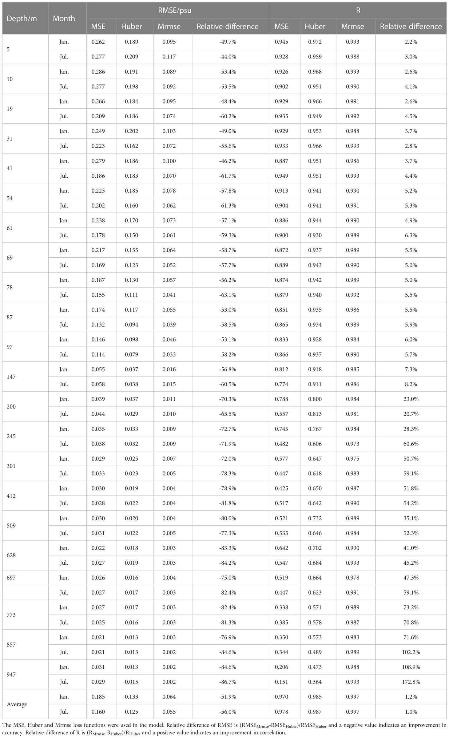
Table 1 RMSE and correlation coefficient (R) between Attention U-net estimated salinity and GLORYS2V4 reanalysis in the upper 1000 m of the SCS in January and July.

FIGURE 3

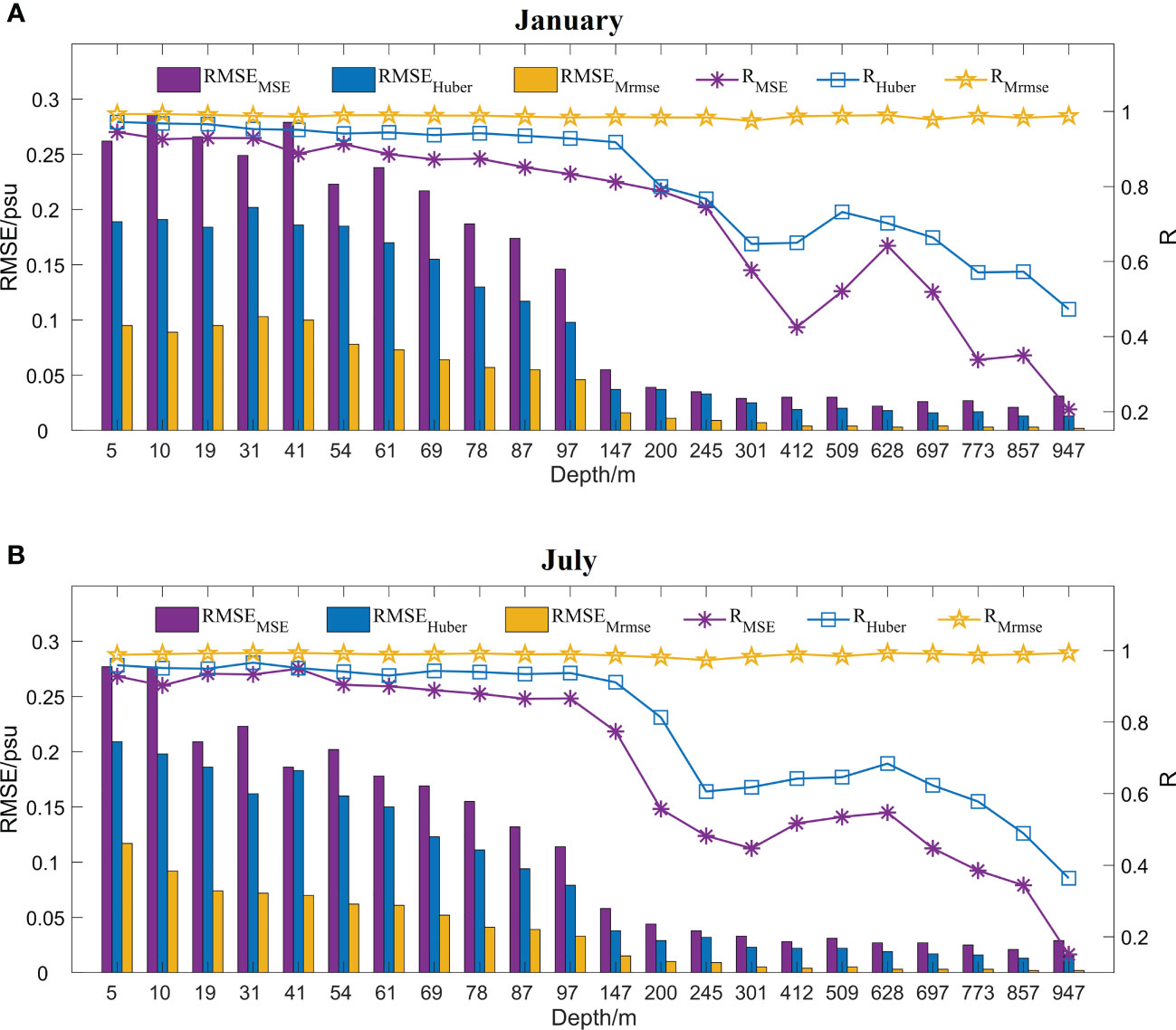
Figure 3 Variations of RMSE and correlation coefficient (R) between Attention U-net estimated salinity and GLORYS2V4 reanalysis as a function of water depth in the SCS in January (A) and July (B). The subscripts “MSE”, “Huber” and “Mrmse” of RMSE and R represent the estimation derived from the model based on MSE, Huber and Mrmse loss functions, respectively.

In contrast, the Mrmse loss function only calculates the errors between the estimation and ground truth at valid data points without consideration of outliers. When the Mrmse loss function is used, the model yields the most accurate construction results, especially in deeper waters. The RMSE at different vertical layers between the labelled and estimated salinity is half or even less than 85% of the error obtained by using the Huber loss function. The error decreases significantly as the water depth increases and the minimum value is 0.002 psu at 947 m depth. Meanwhile, the correlation coefficient is significantly increased from 23.0% to 108.9% in waters deeper than 200 m and its value remains above 0.975. It is marginally larger in the upper waters and changes slightly with the water depth. Similar results were obtained for the model in July (Table 1 and Figure 3B), where the RMSE has a large reduction between 44.0% and 86.7% and the correlation coefficient has a significant increase of 2.8% to 172.8% at different depths. This shows that the Mrmse loss function works better than the MSE or Huber loss function for 3D salinity reconstruction in the SCS. The Huber loss function greatly reduces the attention on the anomaly values, however, it is still not effective for the establishment of 3D salinity reconstruction model in the SCS, because invalid data always exist due to uneven distribution of topography. These invalid data regarded as outliers would induce noise in the training dataset and thus provide false data features, which may lead to unsatisfactory performance of the reconstruction model. On the other hand, the salinity changes slightly within a month. In this case, different features learned by the network are relatively few, and hence false features would have a considerable negative impact on the model performance. The influence of outliers on the model is particularly great in the deeper layers because the number of real salinity data will decrease with depth. When evaluating model errors between estimation and labels over the study domain, the model will learn unnecessary features from the outliers and pay relatively less attention to the useful information of the valid data. Ignoring outliers in the loss function can help the model efficiently learn the characteristics of the real salinity field and yield an estimation close to the ground truth. The generalization ability of the model can be significantly improved as well. Thus, the introduction of the Mrmse loss function in the Attention U-net model has effectively improved the accuracy of salinity reconstruction result at all layers, especially in deeper waters of the SCS.

3.2 Overall performance of Attention U-net model

Based on the comparative experiment results, we finally established the 3D salinity reconstruction model by month for each vertical layer, in which the Mrmse loss function was used. In this section, we evaluated the performance of these models by comparing the model results with GLORYS2V4 reanalysis and in situ mooring measurements, respectively.

3.2.1 Estimated salinity vs. GLORYS2V4 reanalysis

The overall RMSE and correlation coefficient between estimation and the reanalysis in each layer is shown in Table 2. As the water depth increases, the RMSE rapidly decreases from 0.106 psu near the surface to 0.009 psu at 200 m depth. After that, it continues to decline and reaches a minimum value of 0.002 psu in waters deeper than 773 m. The vertical variation of the correlation coefficient is notably different than the RMSE. It remains stable at high values between 0.983 and 0.994. The estimation of testing samples at all depths and over all month has an average RMSE of 0.051 psu and a correlation coefficient of 0.998, suggesting an impressive performance in reconstructing 3D salinity field in the SCS. The RMSE is less than 0.03 psu in areas deeper than 100 m all year round (Figure 4). Relatively larger values are distributed in the upper 100 m layers of the SCS, but are still less than 0.14 psu, and the RMSE in the upper layers shows a seasonal difference. The vertical spatial variation pattern of RMSE is consistent with the results of Meng et al. (2022) in the Pacific Ocean using CNN model. The correlation coefficient always remains high above 0.965, and rarely changes between seasons. However, the value is a little lower in the water layers between 200 m and 400 m. This might be related to the higher variability of salinity at these depths.

TABLE 2

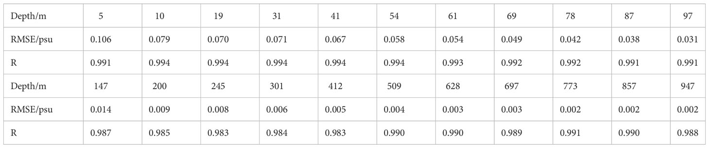
Table 2 RMSE and correlation coefficient (R) between Attention U-net estimated salinity and GLORYS2V4 reanalysis for each layer in the upper 1000 m of the SCS.

FIGURE 4

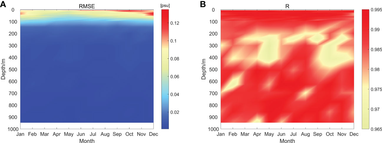
Figure 4 Variation of RMSE (A) and correlation coefficient (R) (B) between Attention U-net estimated salinity and GLORYS2V4 reanalysis with water depth and month.

We further calculated the number of salinity points in the testing dataset at intervals of 0.001 psu, divided it by the total number of the testing data, and then normalized it to a range of 0 to 1 to obtain the density of data points in each interval. Figure 5 shows the density scatterplots between the salinity derived from satellite observed variables and GLORYS2V4 reanalysis at different depths. One can see that most of the statistics are distributed along the isoline where the estimated salinity is equal to the true value, demonstrating that the Attention U-net model performs quite well. The points are concentrated in a wider salinity range of 33.3 psu to 34.2 psu at the depth of 54 m, and at a smaller range for deeper layers. This might be related to the relatively large variation of salinity in the upper SCS. As shown in the left panel of Figure 6, the spatial variability of salinity field is indeed more significant in shallower waters. The maximum horizontal difference is about 2.1 psu at 54 m depth but is only 0.3 psu at depth more than 500 m. Figure 6 also shows that the salinity field estimated from the Attention U-net model has a spatial distribution pattern highly consistent with the GLORYS2V4 reanalysis. The fresher waters within the 100 m depth are widely distributed in the southern SCS, while those at the depth of 509 m are mainly located in the west of the Luzon Strait. The estimation error is close to 0 in almost the whole SCS, especially in the deeper layers. However, errors are slightly larger in a few areas.

FIGURE 5

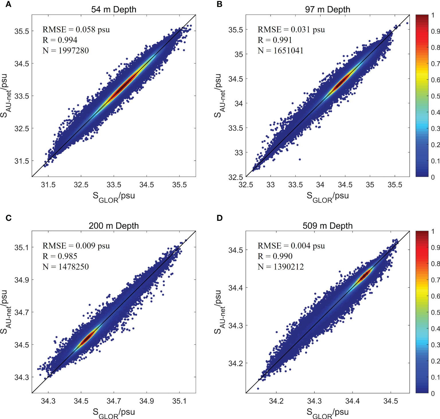
Figure 5 Density scatterplots between the Attention U-net model estimated salinity (S_AU-net) and GLORYS2V4 reanalysis (S_GLOR) at the depth of (A) 54 m, (B) 97 m, (C) 200 m and (D) 509 m in the SCS. The black line indicates the 1-to-1 line. N is the number of data points in all testing samples.

FIGURE 6

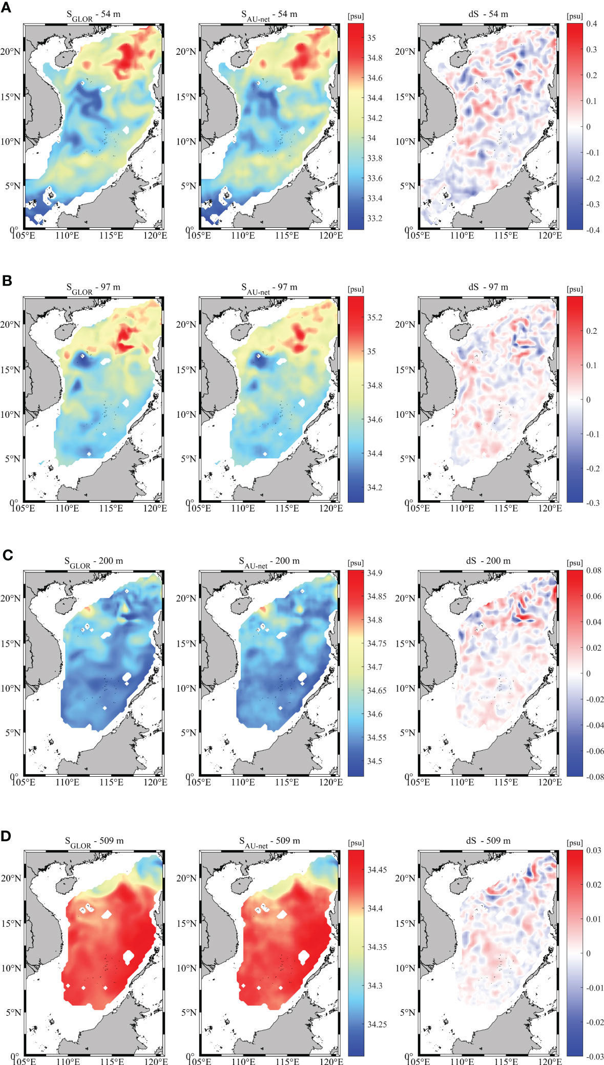
Figure 6 Distribution of salinity field estimated by the Attention U-net model compared to the GLORYS2V4 reanalysis and their difference (dS = S_AU-net – S_GLOR) at the depth of (A) 54 m, (B) 97 m, (C) 200 m and (D) 509 m in the SCS on 1 May 2018.

3.2.2 Estimated salinity vs. in situ measurements

Field measurements can provide reliable ocean salinity profile data, although these data are sparse in space. We collected the salinity data observed by a mooring chain consisting of eight Conductivity-Temperature-Depth (CTD) instruments deployed at 20.54°N, 115.57°E in the northern SCS (Figure 1A). The mooring measures underwater salinity and temperature in depth from about 50 m to 380 m. The salinity profiles from July 11 to 25 2016 were used to further evaluate the accuracy of the reconstructed salinity results. The daily reconstructed salinity profile and its evolution are in good agreement with the mooring observations (Figure 7), further indicating the good performance and applicability of the Attention U-net model. The depth-averaged RMSE between the model estimation and in situ measurements varies from 0.032 psu to 0.066 psu, and the correlation coefficient is greater than 0.94.

FIGURE 7

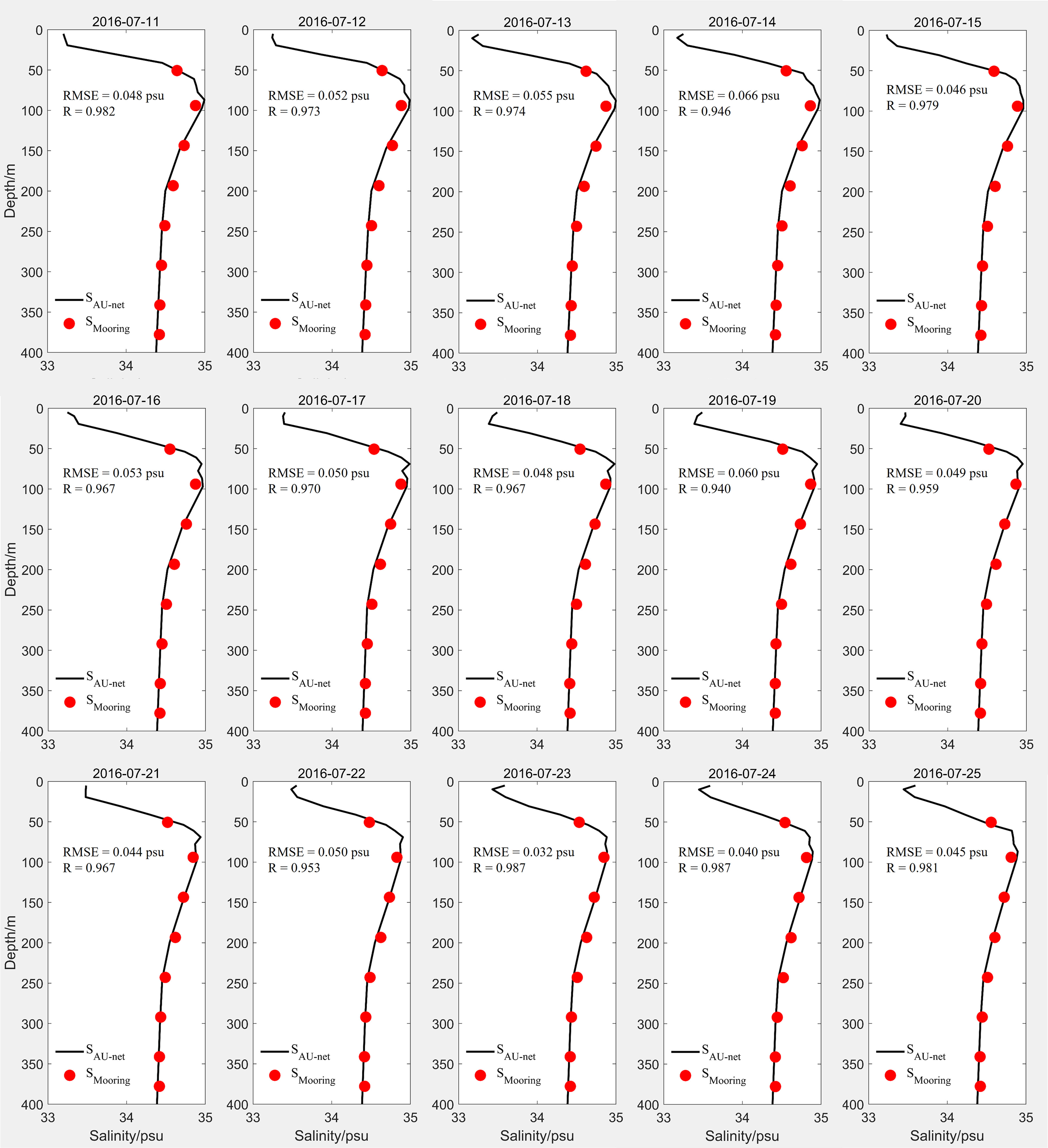
Figure 7 Attention U-net model estimated salinity profiles (S_AU-net) compared to mooring observations (S_Mooring) from July 11 to 25 2016.

4 Discussion

4.1 Error analysis of Attention U-net model

Overall, the Attention U-net model performs quite well in estimating underwater salinity in the SCS and the accuracy is very high in deep waters. The RMSE of the reconstructed salinity in the upper 100 m is slightly larger than that in deeper layers, which may be caused by the more complex salinity structure resulting from active dynamic processes here. The horizontal distribution of the RMSE at three different surface depths is illustrated in Figures 8A–C. At a depth of 5 m, the relatively large error is mainly located in two coastal regions, but their values are still less than 0.3 psu. The regions correspond to the generation and extension of the Pearl River and Mekong River plumes that have a significant impact on the salinity field of the coastal and upper waters of the SCS (Chen et al., 2016; Zeng et al., 2022). The larger error near the Mekong River estuary is particularly notable in the upper 10 m, while the error near the Pearl River estuary is mainly distributed in the top layer. This might be associated with larger pulse of riverine flow into the SCS via the Mekong River, which results in a stronger halocline near the estuary (Gan et al., 2009; Zeng et al., 2022).

FIGURE 8

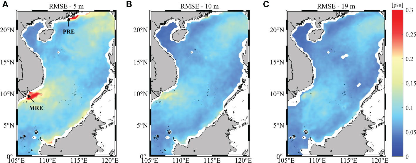
Figure 8 Distribution of RMSE between Attention U-net estimated salinity and GLORYS2V4 reanalysis at the depth of 5 m (A), 10 m (B) and 19 m (C) in the SCS. Black arrows in (A) specify the location of Pearl River estuary (PRE) and Mekong River estuary (MRE), respectively.

Figure 4A shows the upper-layer RMSE between the reconstructed salinity and reanalysis product for all samples in the testing dataset differing between seasons. It is smaller in spring (March-May) and summer (June-August) than in autumn (September-November) and winter (December-February). This seasonal variation is also evident in Figure 9. In summer, the RMSE within the top three layers is larger near the Pearl River and Mekong River estuaries than that in the other parts of the SCS. This might be related to the large amount of river discharge caused by the monsoon and wide extension of the river plumes to the SCS (Ou et al., 2007; Zeng et al., 2022). The southwest monsoon will bring a lot of precipitation over the ocean, thus increasing the river discharge. In winter, rainfall is less due to land breeze, and the corresponding river plume is weaker. As a result, the accuracy of upper-layer salinity reconstruction near the river plumes is much higher than that in summer.

FIGURE 9

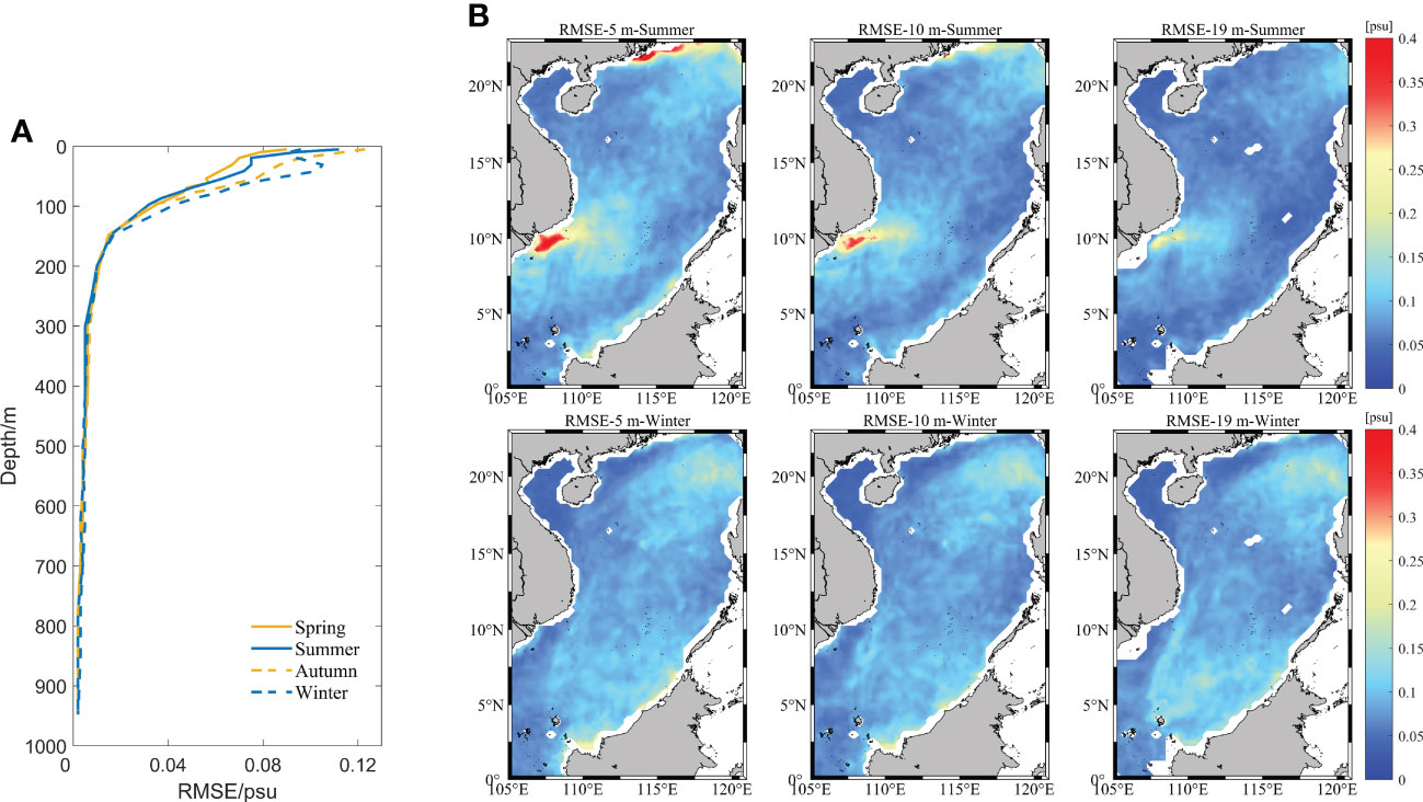
Figure 9 (A) Vertical variation of RMSE between Attention U-net estimated salinity and GLORYS2V4 reanalysis in four seasons. (B) RMSE maps at 5 m, 10 m and 19 m depth of the SCS in summer and winter.

4.2 Broader applications and limitations of salinity reconstruction model

The 0.25°×0.25° gridded satellite observations used as model inputs do not contain many smaller-scale signals which are usually smoothed from the filters in the data processing and might have a significant influence on the accuracy of reconstructed salinity field. To investigate whether the noisy features of sea surface variables would affect the estimation results, an additional group of experiments based on 3D salinity reconstruction model were conducted, in which Gaussian white noise was added to all input satellite data. The results for January are given in Figure 10. After adding noise to surface variables, the Attention U-net model still performs well in 3D salinity reconstruction. The RMSE ranges from 0.002 psu to 0.111 psu and the correlation coefficient is always higher than 0.973, which is close to the results obtained when using smooth data as model inputs. The RMSE in the upper 45 m is slightly larger, but compared to the noiseless case, the maximum increase is less than 0.011 psu. The correlation coefficient shows almost no change at all vertical layers. This indicates that our model is a robust model that can resist some possible noise interference from input data.

FIGURE 10

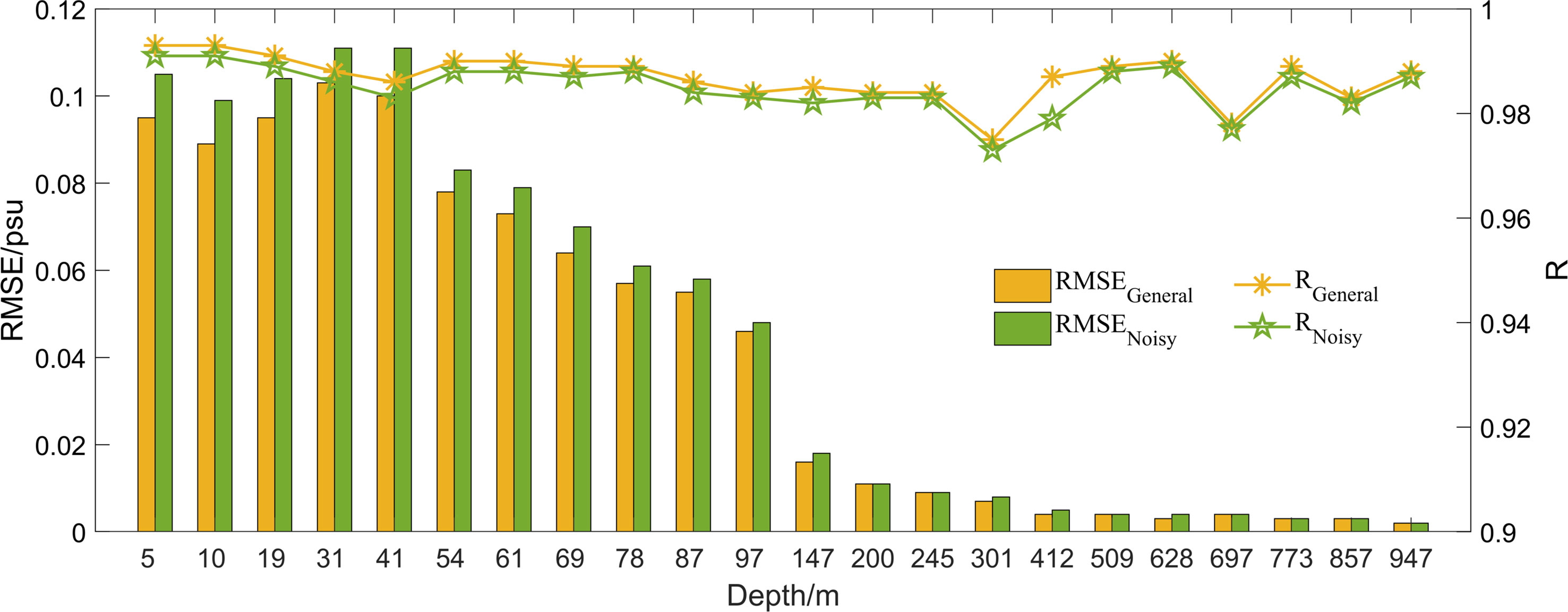
Figure 10 Variations of RMSE and correlation coefficient (R) between Attention U-net estimated salinity and GLORYS2V4 reanalysis as a function of water depth in the SCS in January. The subscripts “General” and “Noisy” of RMSE and R represent the estimation derived from sea surface variables without and with the Gaussian white noise, respectively. The Mrmse loss function is used in the model.

Thus, additional consideration of the river plume to the model input seems to be helpful to improve salinity estimation accuracy (see Section 4.1). However, the runoff discharge data that are usually used to describe the intensity of the river plume are dispersedly distributed on land where 3D salinity data are unavailable, which limits the input of runoff discharge in the model. It is also difficult to obtain these data because most of them are not public. Can we take the effect of river plumes into account indirectly when reconstructing the 3D salinity field in the SCS? This is possible, as SSS information provided by satellites already reflects the impact of river plumes on sea surface properties. To illustrate this, two comparative experiments were conducted to reconstruct 3D salinity fields in the upper 20 m of the SCS from surface variables with and without using SSS, respectively. The RMSE between the estimations and the GLORYS2V4 reanalysis at each vertical layer in summer and winter is given in Table 3. When SSS is added to the model inputs, the horizontally averaged RMSE decreases at each layer, and the maximum decline is 16.4% at a depth of 5 m. A more significant reduction of RMSE appears in summer than winter, while the estimation error near river estuaries is also much larger (see Figure 9B). The influence of SSS on the subsurface salinity reconstruction accuracy in the SCS, especially in the river plume areas, is further investigated using a distribution map of the difference between RMSE derived from surface variables with and without SSS (Figure 11). When SSS is added to the model inputs, the RMSE near the Mekong estuary is significantly reduced in summer and the RMSE around the Pearl River plume also decreases. This indicates that SSS is crucial for 3D salinity reconstruction in the SCS, especially in river plume regions, as it can provide useful information about the impact of river discharge on the salinity. However, the accuracy of satellite-observed SSS is not high enough in coastal areas of the SCS, due to the contamination of land-based radio frequency interference (Zhang et al., 2023). The use of new technologies or satellite sensors to obtain more accurate SSS from satellites will further improve the accuracy of salinity reconstruction in the future.

TABLE 3

Table 3 RMSE between Attention U-net estimated salinity and GLORYS2V4 reanalysis in the upper 20 m of the SCS in summer and winter.

FIGURE 11

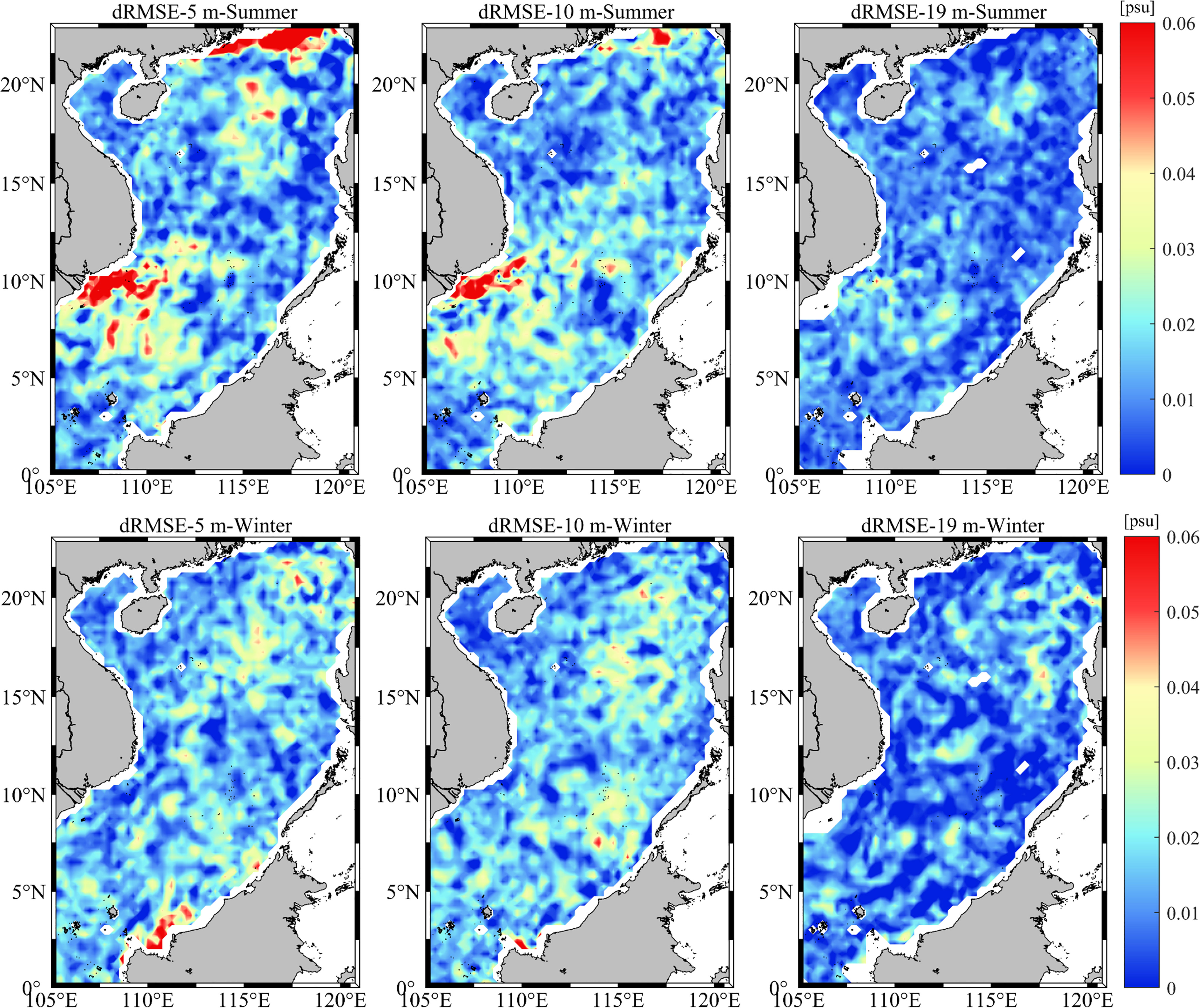
Figure 11 Distribution of differences between RMSE (dRMSE = RMSE₄ –RMSE₅) derived from sea surface variables with and without SSS at 5 m, 10 m and 19 m depth of the SCS in summer and winter.

4.3 Application of reconstructed salinity fields to a mesoscale eddy case study

The high-resolution 3D salinity field estimated from satellite observations using the Attention U-net model can be useful in the study of dynamic processes in the SCS, such as mesoscale eddies. We employ version 3.1 of the altimetric Mesoscale Eddy Trajectories Atlas, supplied by AVISO (https://aviso.altimetry.fr), which contains information of global mesoscale eddies (Mason et al., 2014; Pegliasco et al., 2022). Using this dataset, a mesoscale cyclonic eddy with the radius larger than 100 km was captured in the central SCS. The evolution of the eddy within 5 days from 13 to 17 November 2017 is presented in Figure 12A. The cyclonic eddy propagates northwestward as its shape and internal negative SLA signal slightly change, which means that the eddy may be stable at this stage. Meanwhile, the corresponding SSS anomaly field, obtained by subtracting the SSS from the climatology, is always positive within the eddy during the propagation (Figure 12B). This is associated with upwelling induced by the cyclonic eddy, which lifts the relatively saltier waters at the lower layers to the upper layers and hence increases the salinity at the sea surface. The positive SSS anomaly signal agrees well with the eddy signal detected from the SLA field, though it is slightly smaller. This indicates that the characteristics of the eddy can be at least partially described from the salinity field. Therefore, the reconstructed subsurface salinity anomaly is useful for tracking the evolution of eddy signal beneath the sea surface.

FIGURE 12

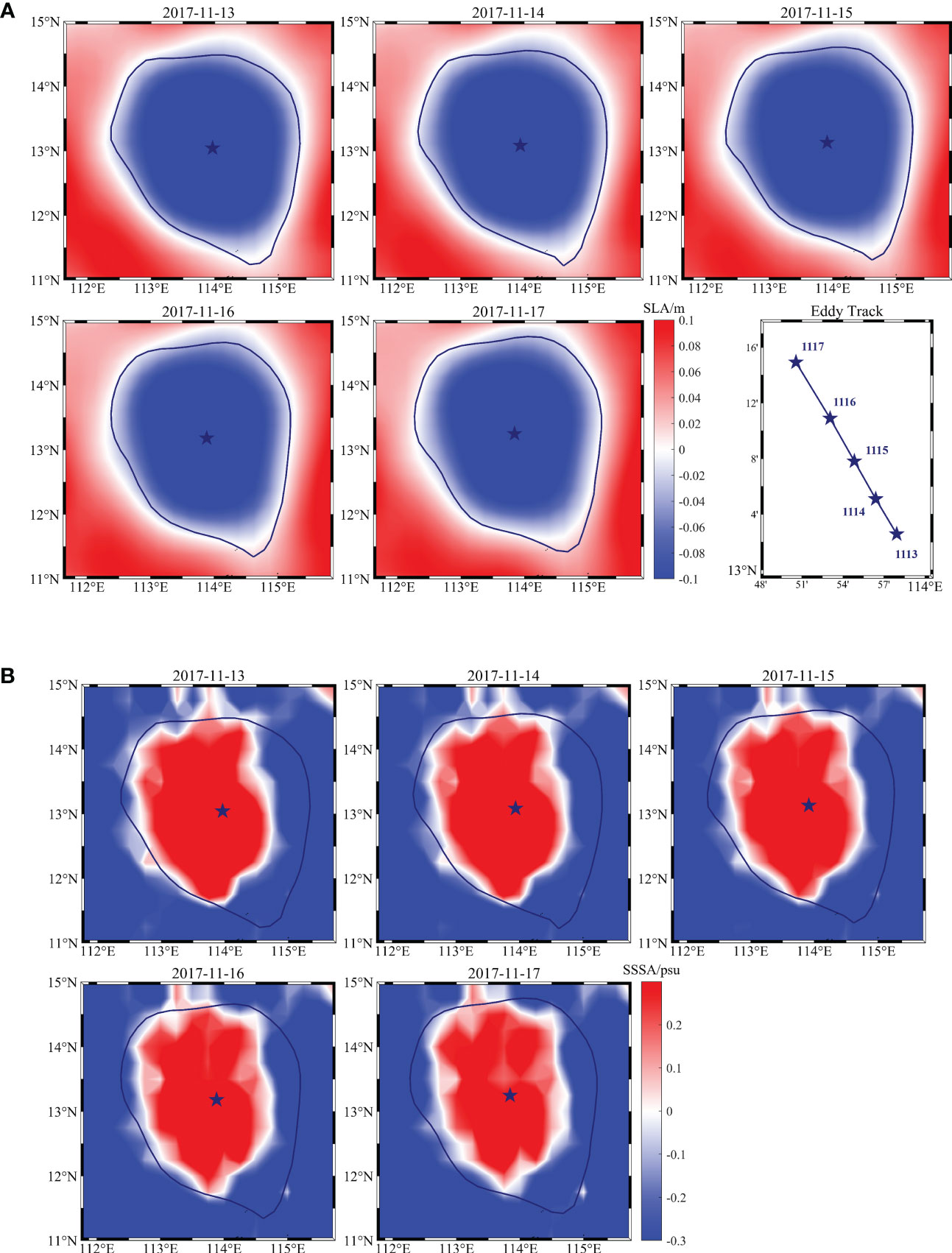
Figure 12 Daily (A) SLA and (B) SSS anomaly map from 13 to 17 November 2017 in the central SCS. The blue star and curve denote the center and contour of the cyclonic eddy, respectively. The movement of the eddy center within 5 days is presented as blue line in (A).

Figure 13 shows a contour map of subsurface salinity anomaly at different water depths (5 m, 10 m, 19 m and 31 m) in the same 5 days. Closed contours of positive subsurface salinity anomaly are present at the top three layers and disappear at a depth of 31 m, suggesting that the subsurface signal of the cyclonic eddy is strong in the upper 19 m. Compared with the surface signal, the underwater signal of eddy also moves towards northwest, but with much smaller radius and lower intensity. Additionally, the underwater center of the cyclonic eddy detected by the subsurface salinity anomaly field is located on the southeast side of that at sea surface captured from the SLA field, revealing the southeastward tilt of eddy axis in the vertical direction (Zhang et al., 2016). The subsurface salinity anomaly field provides a valuable view of the eddy-induced changes in the interior ocean, which will help us comprehensively understand the characteristics of mesoscale eddies in the SCS, especially their vertical structures.

FIGURE 13

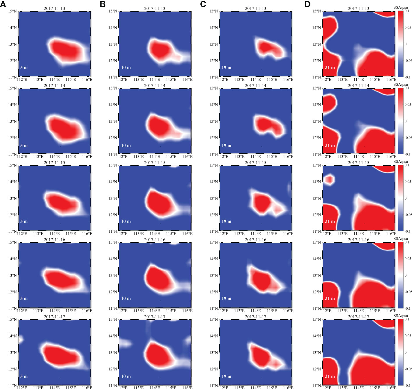
Figure 13 Daily subsurface salinity anomaly map at the depth of (A) 5 m, (B) 10 m, (C) 19 m and (D) 31 m from 13 to 17 November 2017 in the central SCS.

5 Conclusions

The reconstruction of 3D ocean salinity fields is now much easier with the development of numerous remote sensing satellite missions and AI approaches. However, less attention has been paid to underwater salinity estimation in the SCS, where mesoscale and sub-mesoscale phenomena are active, and high-resolution observations are critically needed. We here adopted an Attention U-net model to reconstruct the 3D daily salinity field on a 1/4° grid in the upper 1000 m of the SCS from the satellite observed SSS, SST, SLA and SSW field. In general, the 3D salinity fields of the SCS, at high spatial and temporal resolution, can be well reconstructed. The average RMSE between the estimation results and salinity profiles from the GLORYS2V4 reanalysis product is 0.051 psu and the overall correlation coefficient is 0.998. The RMSE decreases with water depth and reaches a minimum value of 0.002 psu in waters deeper than 773 m, while the correlation coefficient is always higher than 0.983 at all layers. The comparison of salinity reconstruction results with mooring measurements also demonstrates the good performance of the Attention U-net model. In addition, the ability to resist noise interference indicates a strong robustness of the Attention U-net model.

The consideration of topography mask in the loss function is effective in reconstructing more accurate salinity fields in the SCS, especially in deeper waters. When only the estimation errors at valid data points are evaluated in the built model, the RMSE at different vertical layers is half of or even 85% less than the error obtained by using the Huber loss function. The corresponding correlation coefficient is increased by 23.0% to 108.9% in waters deeper than 200 m. Additionally, the use of SSS as model inputs can significantly improve the accuracy of salinity reconstruction in the upper layers of the SCS, especially in river plume regions. When SSS is added to the model inputs, the maximum decline of the RMSE is up to 16.4% at the depth of 5 m. The relatively larger estimation errors are mainly distributed in the coastal and upper waters of the SCS, which may be associated with the active dynamic processes here such as river plumes, as well as the poor quality of SSS satellite products in the coastal regions (González-Gambau et al., 2017; Zhang et al., 2023). The accuracy of coastal satellite SSS products will significantly improve in the near future, which will soon allow more precise reconstructions of 3D salinity fields.

Satellite observed sea surface variables, which determine the resolution of the model output, are of great importance for the 3D ocean salinity reconstruction. However, we can only construct the daily salinity field on a 1/4° grid due to the limitation of present satellite data. Case studies show that the reconstructed salinity structure clearly reveals the underwater signals of mesoscale eddies in the SCS. Observations with higher spatial and temporal resolution can help us better understand the characteristics and evolution of ocean mesoscale or even sub-mesoscale processes. The Surface Water and Ocean Topography (SWOT) mission (Morrow et al., 2019) recently had a successful launch in December 2022. This mission will bring significant future improvement of salinity and wind sensors, and thus we will expect to observe sea surface variables from space with unprecedented resolution and precision. This advance will allow the resolution and accuracy of the 3D temperature and salinity fields to be further improved, which will in turn increase the knowledge of oceanic multi-scale dynamic processes.

Data availability statement

The original contributions presented in the study are included in the article/supplementary material. Further inquiries can be directed to the corresponding author.

Author contributions

Conceptualization: HX and QX. Methodology: HX and QX. Data curation: YC. Formal analysis: HX and KF. Investigation: HX and XY. Visualization: XY and KF. Writing-original draft preparation: HX. Writing-review and editing: QX. Supervision: QX. Funding acquisition: QX, YC and XY. All authors have read and agreed to the published version of the manuscript.

Funding

This work was supported by the National Natural Science Foundation of China under Grants 41976163 and T2261149752 and Guangdong Special Fund Program for Marine Economy Development under Grant GDNRC[2020]050. Hainan Key Research and Development Program under Grant ZDYF2023SHFZ089, Laoshan Laboratory Science and Technology Innovation Projects under Grants LSKJ202201202 and LSKJ202204301.

Conflict of interest

Author Yongcun Cheng was employed by PIESAT Information Technology Co., Ltd.

The remaining authors declare that the research was conducted in the absence of any commercial or financial relationships that could be construed as a potential conflict of interest.

Publisher’s note

All claims expressed in this article are solely those of the authors and do not necessarily represent those of their affiliated organizations, or those of the publisher, the editors and the reviewers. Any product that may be evaluated in this article, or claim that may be made by its manufacturer, is not guaranteed or endorsed by the publisher.

References

Agarwal N., Sharma R., Basu S., Agarwal V. K. (2007). Derivation of salinity profiles in the Indian ocean from satellite surface observations. IEEE Geosci. Remote Sens. Lett. 4 (2), 322–325. doi: 10.1109/lgrs.2007.894163

CrossRef Full Text | Google Scholar

Atlas R., Hoffman R. N., Ardizzone J., Leidner S. M., Jusem J. C., Smith D. K., et al. (2011). A cross-calibrated, multiplatform ocean surface wind velocity product for meteorological and oceanographic applications. B. Am. Meteorol. Soc 92 (2), 157–174. doi: 10.1175/2010bams2946.1

CrossRef Full Text | Google Scholar

Ballabrera-Poy J., Mourre B., Garcia-Ladona E., Turiel A., Font J. (2009). Linear and non-linear T-s models for the eastern north Atlantic from argo data: role of surface salinity observations. Deep Sea Res. Pt. I: Oceanographic Res. Papers 56 (10), 1605–1614. doi: 10.1016/j.dsr.2009.05.017

CrossRef Full Text | Google Scholar

Bao S., Zhang R., Wang H., Yan H., Yu Y., Chen J. (2019). Salinity profile estimation in the pacific ocean from satellite surface salinity observations. J. Atmos. Ocean. Tech. 36 (1), 53–68. doi: 10.1175/jtech-d-17-0226.1

CrossRef Full Text | Google Scholar

Boutin J., Reul N., Koehler J., Martin A., Catany R., Guimbard S., et al. (2021). Satellite-based sea surface salinity designed for ocean and climate studies. J. Geophys. Res.: Oceans 126, 1–28. doi: 10.1029/2021jc017676

CrossRef Full Text | Google Scholar

Buongiorno Nardelli B. (2020). A deep learning network to retrieve ocean hydrographic profiles from combined satellite and in situ measurements. Remote Sens. 12 (3151), 1–14. doi: 10.3390/rs12193151

CrossRef Full Text | Google Scholar

Carnes M. R., Teague W. J., Mitchell J. L. (1994). Inference of subsurface thermohaline structure from fields measurable by satellite. J. Atmos. Ocean. Tech. 11 (2), 551–566. doi: 10.1175/1520-0426(1994)011<0551:IOSTSF>2.0.CO;2

CrossRef Full Text | Google Scholar

CATDS (2017). Data from: CATDS-PDC L3OS 2P-daily valid ocean salinity values product from SMOS satellite. Institut français de recherche pour l'exploitation de la mer (Paris, France: IFREMER). The location is Paris, France. doi: 10.12770/77edd308-4296-4774-b6f3-5b38301cee18

CrossRef Full Text | Google Scholar

Chaudhari S., Mithal V., Polatkan G., Ramanath R. (2021). An attentive survey of attention models. ACM Trans. Intell. Syst. Technol. 12 (5), 1–32. doi: 10.1145/3465055

PubMed Abstract | CrossRef Full Text | Google Scholar

Chen Z., Pan J., Jiang Y. (2016). Role of pulsed winds on detachment of low salinity water from the pearl river plume: upwelling and mixing processes. J. Geophys. Res.: Oceans 121 (4), 2769–2788. doi: 10.1002/2015jc011337

CrossRef Full Text | Google Scholar

Gan J., Li L., Wang D., Guo X. (2009). Interaction of a river plume with coastal upwelling in the northeastern south China Sea. Cont. Shelf Res. 29 (4), 728–740. doi: 10.1016/j.csr.2008.12.002

CrossRef Full Text | Google Scholar

Garric G., Parent L., Greiner E., Drévillon M., Hamon M., Lellouche J.-M., et al. (2017). Performance and quality assessment of the global ocean eddy-permitting physical reanalysis GLORYS2V4 (Vienna, Austria:EGU General Assembly Conference Abstracts). Vienna, Austria.

Google Scholar

González-Gambau V., Olmedo E., Martinez J., Turiel A., Duran I. (2017). Improvements on calibration and image reconstruction of SMOS for salinity retrievals in coastal regions. IEEE J. Sel. Top. Appl. Earth Obs. Remote Sens. 10 (7), 3064–3078. doi: 10.1109/jstars.2017.2685690

CrossRef Full Text | Google Scholar

Guinehut S., Dhomps A. L., Larnicol G., Le Traon P. Y. (2012). High resolution 3-d temperature and salinity fields derived from in situ and satellite observations. Ocean Sci. 8 (5), 845–857. doi: 10.5194/os-8-845-2012

CrossRef Full Text | Google Scholar

Han Y., Ye J. C. (2018). Framing U-net via deep convolutional framelets: application to sparse-view CT. IEEE trans. Med. Imaging 37 (6), 1418–1429. doi: 10.1109/TMI.2018.2823768

CrossRef Full Text | Google Scholar

He Q., Zhan H., Cai S., He Y., Huang G., Zhan W. (2018). A new assessment of mesoscale eddies in the south China Sea: surface features, three-dimensional structures, and thermohaline transports. J. Geophys. Res.: Oceans 123 (7), 4906–4929. doi: 10.1029/2018jc014054

CrossRef Full Text | Google Scholar

Held I. M., Soden B. J. (2006). Robust responses of the hydrological cycle to global warming. J. Clim. 19 (21), 5686–5699. doi: 10.1175/JCLI3990.1

CrossRef Full Text | Google Scholar

Henning C. C., Vallis G. K. (2004). The effects of mesoscale eddies on the main subtropical thermocline. J. Phys. Oceanogr. 34 (11), 2428–2442. doi: 10.1175/JPO2639.1

CrossRef Full Text | Google Scholar

Huang X., Chen Z., Zhao W., Zhang Z., Zhou C., Yang Q., et al. (2016). An extreme internal solitary wave event observed in the northern south China Sea. Sci. Rep. 6 (30041), 1–10. doi: 10.1038/srep30041

PubMed Abstract | CrossRef Full Text | Google Scholar

Huang B., Liu C., Banzon V., Freeman E., Graham G., Hankins B., et al. (2021). Improvements of the daily optimum interpolation sea surface temperature (DOISST) version 2.1. J. Clim. 34 (8), 2923–2939. doi: 10.1175/jcli-d-20-0166.1

CrossRef Full Text | Google Scholar

Keppler L., Cravatte S., Chaigneau A., Pegliasco C., Gourdeau L., Singh A. (2018). Observed characteristics and vertical structure of mesoscale eddies in the southwest tropical pacific. J. Geophys. Res.: Oceans 123 (4), 2731–2756. doi: 10.1002/2017jc013712

CrossRef Full Text | Google Scholar

Klemas V., Yan X.-H. (2014). Subsurface and deeper ocean remote sensing from satellites: an overview and new results. Prog. Oceanogr. 122, 1–9. doi: 10.1016/j.pocean.2013.11.010

CrossRef Full Text | Google Scholar

Lagerloef G. S. E. (2002). Introduction to the special section: the role of surface salinity on upper ocean dynamics, air-sea interaction and climate. J. Geophys. Res.: Oceans 107, 1–2. doi: 10.1029/2002jc001669

CrossRef Full Text | Google Scholar

Li X., Liu B., Zheng G., Ren Y., Zhang S., Liu Y., et al. (2020). Deep-learning-based information mining from ocean remote-sensing imagery. Natl. Sci. Rev. 7 (10), 1584–1605. doi: 10.1093/nsr/nwaa047

PubMed Abstract | CrossRef Full Text | Google Scholar

Li X., Zhou Y., Wang F. (2022). Advanced information mining from ocean remote sensing imagery with deep learning. J. Remote Sens. 2022, 1–4. doi: 10.34133/2022/9849645

CrossRef Full Text | Google Scholar

Mason E., Pascual A., McWilliams J. C. (2014). A new sea surface height-based code for oceanic mesoscale eddy tracking. J. Atmos. Ocean. Tech. 31 (5), 1181–1188. doi: 10.1175/jtech-d-14-00019.1

CrossRef Full Text | Google Scholar

Mears C. A., Scott J., Wentz F. J., Ricciardulli L., Leidner S. M., Hoffman R., et al. (2019). A near-real-time version of the cross-calibrated multiplatform (CCMP) ocean surface wind velocity data set. J. Geophys. Res.: Oceans 124 (10), 6997–7010. doi: 10.1029/2019jc015367

CrossRef Full Text | Google Scholar

Meissner T., Wentz F. J., Manaster A., Lindsley R. (2019). Data from: remote sensing systems SMAP ocean surface salinities [level 2C], version 4.0 validated release s. r. doi: 10.5067/SMP40-2SOCS

CrossRef Full Text | Google Scholar

Meissner T., Wentz F. J., Vine D. M. L. (2018). The salinity retrieval algorithms for the NASA aquarius version 5 and SMAP version 3 releases. Remote Sens. 10 (7), 1–25. doi: 10.3390/rs10071121

CrossRef Full Text | Google Scholar

Meng L., Yan C., Zhuang W., Zhang W., Geng X., Yan X.-H. (2022). Reconstructing high-resolution ocean subsurface and interior temperature and salinity anomalies from satellite observations. IEEE Trans. Geosci. Remote Sens. 60, 1–14. doi: 10.1109/tgrs.2021.3109979

CrossRef Full Text | Google Scholar

Morrow R., Fu L.-L., Ardhuin F., Benkiran M., Chapron B., Cosme E., et al. (2019). Global observations of fine-scale ocean surface topography with the surface water and ocean topography (SWOT) mission. Front. Mar. Sci. 6 (232). doi: 10.3389/fmars.2019.00232

CrossRef Full Text | Google Scholar

Oktay O., Schlemper J., Folgoc L. L., Lee M., Heinrich M., Misawa K., et al. (2018). “Attention U-net: learning where to look for the pancreas,” in Conference on Medical Imaging with Deep Learning, Amsterdam, The Netherlands.

Google Scholar

Ou S., Zhang H., Wang D., He J. (2007). Horizontal characteristics of buoyant plume off the pearl river estuary during summer. J. Coast. Res. 50, 652–657.

Google Scholar

Pegliasco C., Delepoulle A., Morrow R., Faugère Y., Dibarboure G. (2022). META3.1exp: a new global mesoscale eddy trajectories atlas derived from altimetry. Earth Syst. Sci. Data 14 (3), 1087–1107. doi: 10.5194/essd-2021-300

CrossRef Full Text | Google Scholar

Ren L., Riser S. C. (2010). Observations of decadal time scale salinity changes in the subtropical thermocline of the north pacific ocean. Deep Sea Res. Pt. II: Topical Stud. Oceanography 57 (13), 1161–1170. doi: 10.1016/j.dsr2.2009.12.005

CrossRef Full Text | Google Scholar

Reynolds R. W., Smith T. M., Liu C., Chelton D. B., Casey K. S., Schlax M. G. (2007). Daily high-resolution-blended analyses for sea surface semperature. J. Clim. 20 (22), 5473–5496. doi: 10.1175/2007jcli1824.1

CrossRef Full Text | Google Scholar

Ronneberger O., Fischer P., Brox T. (2015). “U-Net: convolutional networks for biomedical image segmentation,” in Medical image computing and computer-assisted intervention-MICCAI (Cham, Switzerland: Springer).

Google Scholar

Schmidtko S., Stramma L., Visbeck M. (2017). Decline in global oceanic oxygen content during the past five decades. Nat 542 (7641), 335–339. doi: 10.1038/nature21399

CrossRef Full Text | Google Scholar

Schmitt R. W. (2008). Salinity and the global water cycle. Oceanogr 21 (1), 12–19. doi: 10.5670/oceanog.2015.03

CrossRef Full Text | Google Scholar

Song T., Wei W., Meng F., Wang J., Han R., Xu D. (2022). Inversion of ocean subsurface temperature and salinity fields based on spatio-temporal correlation. Remote Sens. 14 (11), 1–23. doi: 10.3390/rs14112587

CrossRef Full Text | Google Scholar

Su H., Yang X., Lu W., Yan X.-H. (2019). Estimating subsurface thermohaline structure of the global ocean using surface remote sensing observations. Remote Sens. 11 (1598), 1–22. doi: 10.3390/rs11131598

CrossRef Full Text | Google Scholar

Wang G., Su J., Chu P. C. (2003). Mesoscale eddies in the south China Sea observed with altimeter data. Geophys. Res. Lett. 30 (21), 1–6. doi: 10.1029/2003gl018532

CrossRef Full Text | Google Scholar

Woo S., Park J., Lee J.-Y., Kweon I. S. (2018). “CBAM: convolutional block attention module,” in Europeon conference on computer vision (Cham, Switzerland: Springer).

Google Scholar

Xie H., Xu Q., Cheng Y., Yin X., Jia Y. (2022a). Reconstruction of subsurface temperature field in the south China Sea from satellite observations based on an attention U-net model. IEEE Trans. Geosci. Remote Sens. 60, 1–19. doi: 10.1109/tgrs.2022.3200545

CrossRef Full Text | Google Scholar

Xie H., Xu Q., Zheng Q.a., Xiong X., Ye X., Cheng Y. (2022b). Assessment of theoretical approaches to derivation of internal solitary wave parameters from multi-satellite images near the dongsha atoll of the south China Sea. Acta Oceanol. Sin. 41 (2), 1–9. doi: 10.1007/s13131-022-2015-3

CrossRef Full Text | Google Scholar

Xu K., Ba J., Kiros R., Cho K., Courville A., Salakhutdinov R., et al. (2015). “Show, attend and tell: neural image caption generation with visual attention,” in Proceedings of the International Conference on Machine Learning, Lille, France.

Google Scholar

Yang T., Chen Z., He Y. (2015). A new method to retrieve salinity profiles from sea surface salinity observed by SMOS satellite. Acta Oceanol. Sin. 34 (9), 85–93. doi: 10.1007/s13131-015-0735-3

CrossRef Full Text | Google Scholar

Zeng X., Bracco A., Tagklis F. (2022). Dynamical impact of the Mekong river plume in the south China Sea. J. Geophys. Res.: Oceans 127 (5), 1–15. doi: 10.1029/2021jc017572

CrossRef Full Text | Google Scholar

Zhang Z., Tian J., Qiu B., Zhao W., Chang P., Wu D., et al. (2016). Observed 3D structure, generation, and dissipation of oceanic mesoscale eddies in the south China Sea. Sci. Rep. 6 (1), 24349. doi: 10.1038/srep24349

PubMed Abstract | CrossRef Full Text | Google Scholar

Zhang S., Xu Q., Wang H., Kang Y., Li X. (2022). Automatic waterline extraction and topographic mapping of tidal flats from SAR images based on deep learning. Geophys. Res. Lett. 49, 1–13. doi: 10.1029/2021gl096007

PubMed Abstract | CrossRef Full Text | Google Scholar

Zhang L., Zhang Y., Yin X. (2023). Aquarius sea surface salinity retrieval in coastal regions based on deep neural networks. Remote Sens. Environ. 284. (113357), 1–15. doi: 10.1016/j.rse.2022.113357

CrossRef Full Text | Google Scholar

Zheng Q. A., Susanto R. D., Ho C.-R., Song Y. T., Xu Q. (2007). Statistical and dynamical analyses of generation mechanisms of solitary internal waves in the northern south China Sea. J. Geophys. Res. 112, 1–16. doi: 10.1029/2006jc003551

CrossRef Full Text | Google Scholar

Zine S., Boutin J., Font J., Reul N., Waldteufel P., Gabarro C., et al. (2008). Overview of the SMOS sea surface salinity prototype processor. IEEE Trans. Geosci. Remote Sens. 46 (3), 621–645. doi: 10.1109/tgrs.2008.915543

CrossRef Full Text | Google Scholar