Remote sensing and machine learning method to support sea surface pCO2 estimation in the Yellow Sea

1 Introduction

The rapid growth of fossil fuel usage and industry has increased the atmospheric carbon dioxide (CO₂) concentration by approximately 40% since the Industrial Revolution (Landschützer et al., 2014; Friedlingstein et al., 2022). Global oceans absorb 30% of the CO₂ released by industry and human activities and they are a significant sink for atmospheric CO₂. Coastal seas cover 7% of the oceanic surface area but the sea-air exchange carbon fluxes (FCO₂) comprise approximately 25–50% of the global oceans (Laruelle et al., 2018), and thus they play important roles in absorbing atmospheric CO₂ (Dai et al., 2022). Due to the effects of the complex physical environment and biological activities, great errors occur in estimations of FCO₂ in coastal seas (Landschützer et al., 2018; Mignot et al., 2022). Therefore, estimating sea surface carbon dioxide partial pressure (pCO₂) accurately for coastal seas is critical for precisely estimating the global FCO₂ (Laruelle et al., 2018).

In general, pCO₂ is regulated by thermodynamic effects, biogeochemical effects, mixing effects, and air–sea exchange effects (Liu et al., 2019; Ye et al., 2022). Some environmental variables can characterize these four effects. In particular, the sea surface temperature (SST, °C) directly reflects thermodynamic effects, while the chlorophyll concentration (Chl, mg m⁻³) and diffuse attenuation of downwelling irradiance (Kd, m⁻¹) can indicate biogeochemical effects on the surface pCO₂. In addition, the SST, salinity (SSS, psu), and mixed layer depth (MLD, m) are closely related to mixing effects, and the wind speed can characterize the sea–air exchange process (Gu et al., 2021).

Due to their unique advantage in terms of high spatiotemporal resolution, satellite approaches are efficient for observing pCO₂. In previous studies, both semi-analytical (Hales et al., 2012; Bai et al., 2015; Chen et al., 2017) and empirical approaches (Lohrenz et al., 2010; Tao et al., 2012; Qin et al., 2014; Chen et al., 2016; Chen et al., 2019; Fu et al., 2020) were used to estimate the sea surface pCO₂. Many studies have used satellite data to estimate the sea surface pCO₂, but recent studies also examined and compared the capability of semi-analytical and empirical algorithms for estimating the coastal pCO₂ (Chen et al., 2017; Chen et al., 2019). However, the high spatiotemporal variability and diversity of pCO₂, the inaccuracy of satellite data, and limited availability of in-situ pCO₂ data from coastal seas make it challenging to establish a model of pCO₂. Several efforts have been made to construct various algorithms or models, but the satellite-derived pCO₂ in coastal seas generally has higher uncertainty than that for open seas, and the root mean square difference (RMSD) can be as high as 90 μatm (Chen et al., 2019).

The Yellow Sea (YS) is an important coastal sea in the west Pacific Ocean. The pCO₂ in the YS has considerable seasonal variations and an unbalanced spatial distribution (Wang and Zhai, 2021). For example, extremely high pCO₂ values have been observed during the summer in the center of the YS, whereas extremely low pCO₂ values have been observed in the southwestern YS (Qu et al., 2014; Zhai, 2018). Since the 1980s, many studies have investigated carbonate, pCO₂, and FCO₂ in the YS (Xue et al., 2011; Qu et al., 2014; Zhai et al., 2014; Zhai, 2018; Choi et al., 2019; Deng et al., 2021). However, accurately quantifying pCO₂ and FCO₂ in the YS remains a challenge. In particular, Wang and Zhai (2021) indicated that the YS is a carbon sink and FCO₂ is about –0.5 ± 1.9 mol m⁻² year⁻¹, whereas Qu et al. (2014) suggested that the YS is a carbon source. In addition, the physical and biological conditions in coastal seas have changed due to rapid climate change. For example, SST and Chl have increased (Liu et al., 2021; Lu et al., 2021). These variations will have influenced the changes in the sea surface pCO₂. Indeed, recent studies showed that the CO₂ absorption rates increased in some coastal seas (Li and Zhai, 2019; Xiong et al., 2020). To the best of our knowledge, no previous studies have quantified the long-term trend in the carbon absorption capacity of the YS due to the lack of in-situ pCO₂ data over the entire YS. Thus, in order to accurately quantify the pCO₂ in the YS and understand the response of the pCO₂ to global climate change, we developed an inversion model of pCO₂ in the YS in the present study. Two previous remote sensing studies investigated the pCO₂ in the YS (Tao et al., 2012; Qin et al., 2014), and both used in-situ SST and Chl data to establish multiple polynomial regression (MPR) models. This modeling method is simple but the errors are large. Therefore, in the present study, we aimed: (1) to develop machine learning models for accurately deriving pCO₂ from satellite remote sensing data; and (2) to analyze the long-term trend in the pCO₂ during 2003–2021 in the YS.

2 Materials and methods

2.1 Study area

The YS is a semi-enclosed shelf shallow sea (29.5°N–40.5°N, 118.5°E–126.5°E) located west of the Liaodong Peninsula and east of the Korean Peninsula (Figure 1). The mean water depth is 44 m (Liu et al., 2009). The areas and depths of the North Yellow Sea (NYS) and South Yellow Sea (SYS) are 70 × 10³ km² and 38 m, and 300 × 10³ km² and 44 m, respectively. The climate and ocean circulations exhibit strong seasonality due to the effect of the East Asian Monsoon (Ding et al., 2018). In the winter, the YS is mainly influenced by the Yellow Sea Warm Current (YSWC) and the Yellow Sea Coastal Current. The Yellow Sea Warm Current invades the YS from south to north, and brings warm ocean water to the YS, which makes some regions into carbon sources in the YS (Xue et al., 2011). In the summer, the central YS is occupied by the Yellow Sea Cold Water Mass (YSCWM) and there is a strong thermocline above the YSCWM. In addition, the northeastern extension of the Changjiang Dilution Water (CDW) carries a considerable amount of nutrients to the west of the SYS, and this region sustains high phytoplankton production, thereby leading to lower pCO₂ values (Qu et al., 2014). Overall, the YS current is an important factor that affects pCO₂. A previous study showed that the coastal currents in the YS have strengthened in recent years (Liu S, et al., 2023), which may affect the interannual variation in the pCO₂ in the YS.

FIGURE 1

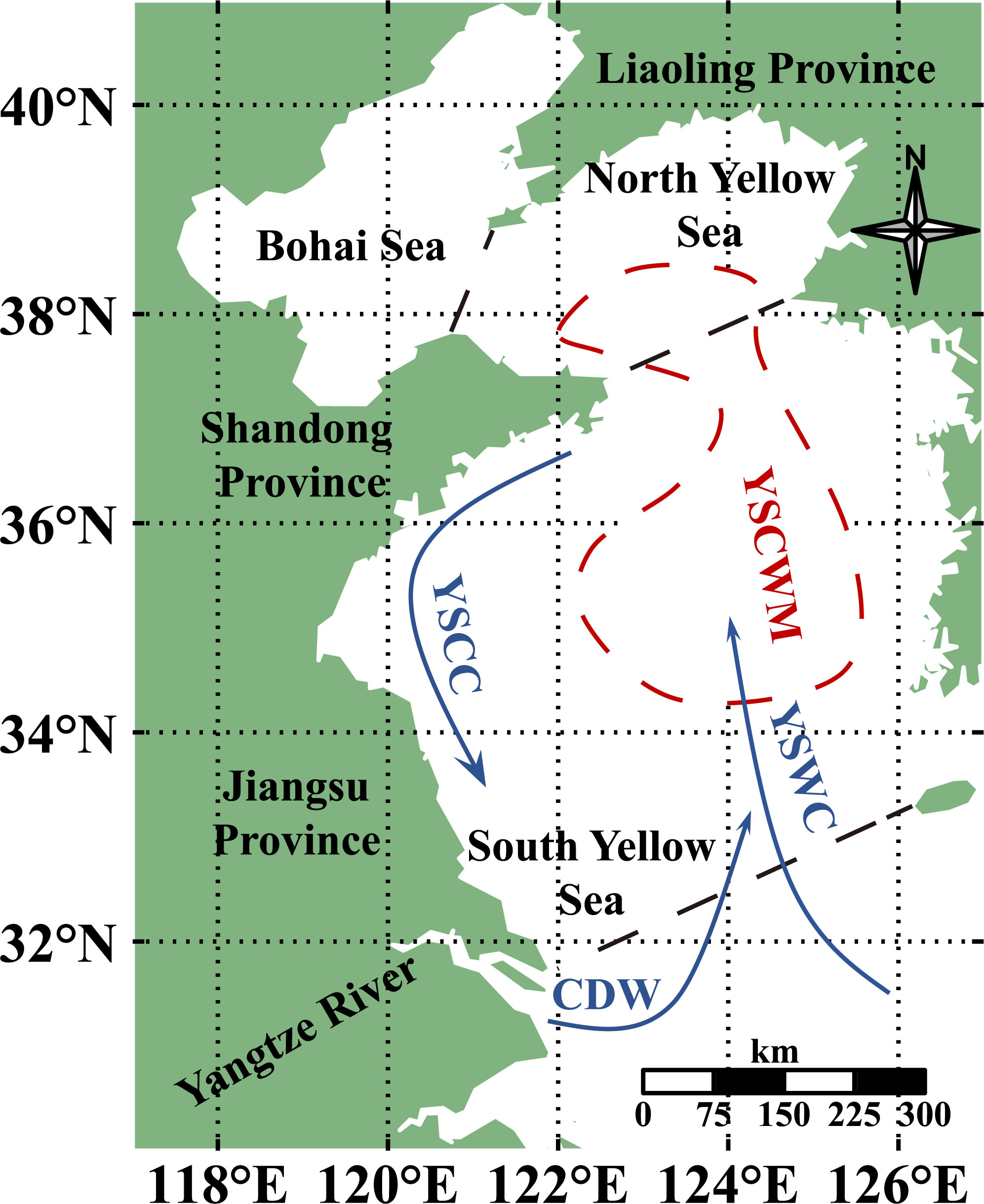
Figure 1 Chart of the study region. The three black dashed lines represent the boundaries between the North Yellow Sea (NYS) and Bohai Sea, the NYS and South Yellow Sea (SYS), and the SYS and East China Sea (ECS).

The YS is surrounded by rapidly developing economic regions, and the rapid development of mariculture has caused severe environmental problems, such as phytoplankton blooms and changes in ocean acidification. Therefore, the carbon cycle process in the YS is managed by both the coastal hydrodynamics and human activities (Choi et al., 2019).

2.2 Data sets

We collected fugacity of CO₂ (fCO₂) data from 14 cruises conducted between 2011 and 2019, which homogenously covered the entire annual cycle (Table 1). Data were derived from four cruises conducted in 2019 by Yu et al. (2022), and data collected from 10 other cruises by Wang and Zhai (2021).

fCO₂ was conversed into pCO₂ using the following formula (1):

$\begin{array}{ll}fC{O}_2=pC{O}_2·\exp \left(p·\frac{B+2\sigma }{RT}\right)& (1)\end{array}$

where p is the total pressure (Pa), R is a gas constant (8.314 J K⁻¹ mol⁻¹), T is the absolute temperature of the sea surface (K), and B and σ are rectification coefficients, which are calculated with formulas (2) and (3).

$\begin{array}{ll}\text{B}=(-1636.75+12.0408\times \text{T}-3.27957\times {10}^{-2}{\text{T}}^2+3.16528\times {10}^{-5}{\text{T}}^3)\times {10}^{-6}& (2)\end{array}$

$\begin{array}{ll}\text{σ}=(57.7-0.118\text{T})\times {10}^{-6}& (3)\end{array}$

The inverse model of pCO₂ in the YS was established with Chl, SST, SSS, and Kd as input variables. In addition, Julday (Jday, or day of year) was selected as an input to highlight the periodical changes in pCO₂ (Lefevre et al., 2005; Signorini et al., 2013). Chl and Kd, SST, and SSS were used to represent biochemical, thermodynamic, and mixing effects on the sea surface pCO₂, respectively. Level 3 8-days and monthly SST (°C), Chl (mg m⁻³), and Kd (m⁻¹) data sets were obtained from Moderate Resolution Imaging Spectroradiometer (MODIS)-Aqua for January 2003 and December 2021 (https://oceancolor.gsfc.nasa.gov/) at a spatial resolution of 4 km. SSS data observed directly by ocean color sensor satellites are not available, so in-situ SSS data were used to develop the model in this study. The HYbrid Coordinate Ocean Model (HYCOM) SSS data set (monthly products with a 4-km resolution) was selected to derive maps of the sea surface pCO₂ (available from: https://www.hycom.org/). In addition, the gridded atmospheric pCO₂ $(pC{O}_2^{air})$ data set (daily, with a spatial resolution of 2° × 2.5°) provided by Rödenbeck et al. (2013) was used (available from: http://www.bgc-jena.mpg.de/SOCOM/).

Due to the influence of cloud cover, sensor technology, atmospheric correction algorithms, and other factors, satellite remote sensing data have a high missing rate in time and space. Therefore, satellite data were interpolated using Data Interpolating Empirical Orthogonal Functions (DINEOF) to obtain more matching pairs. A pixel located at 122°E and 33.2°N was selected to verify the rationality of the reconstructed data. The reconstructions agreed with the original data and complemented the missing data well (Figure 2).

FIGURE 2

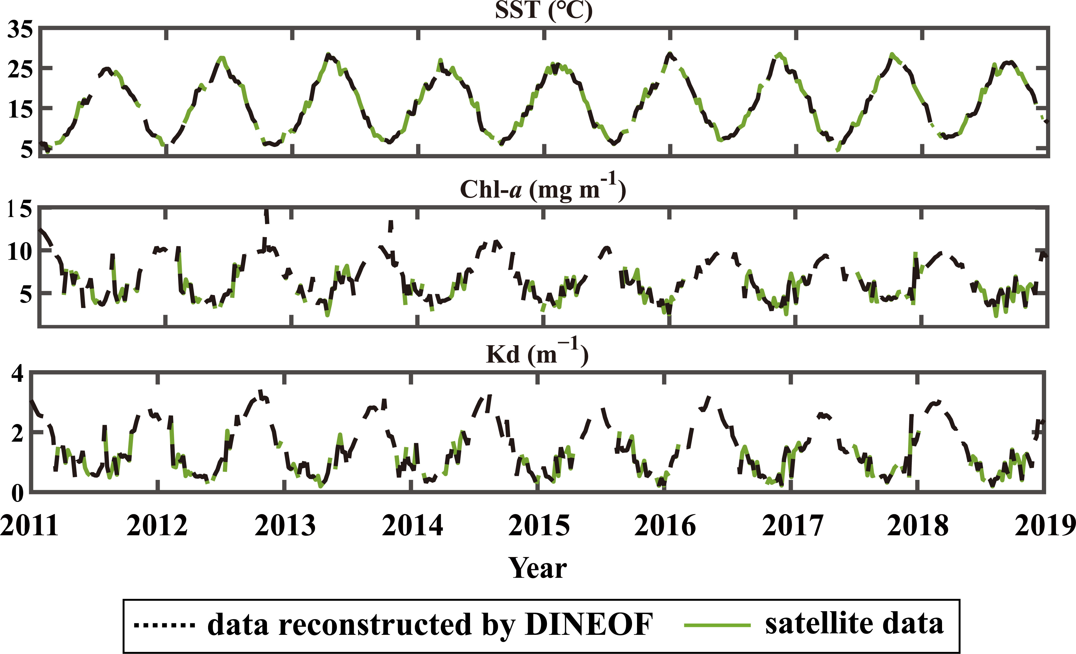
Figure 2 Comparison of reconstructed and original data.

Satellite data were matched with in-situ data according to (Le et al., 2019). Briefly, a time window of ± 8 days was applied between the in-situ and satellite-derived data. In addition, in order to filter sensor and algorithm noise, the median of a 3 × 3-pixel box was focused on every sample point. If the coefficient of variation for the effective pixels in the 3 × 3-pixel box was ≤ 0.4, the extracted data were used to develop the model together with the in-situ data. Finally, we obtained 638 matched pairs from 14 cruises (Figure 3).

FIGURE 3

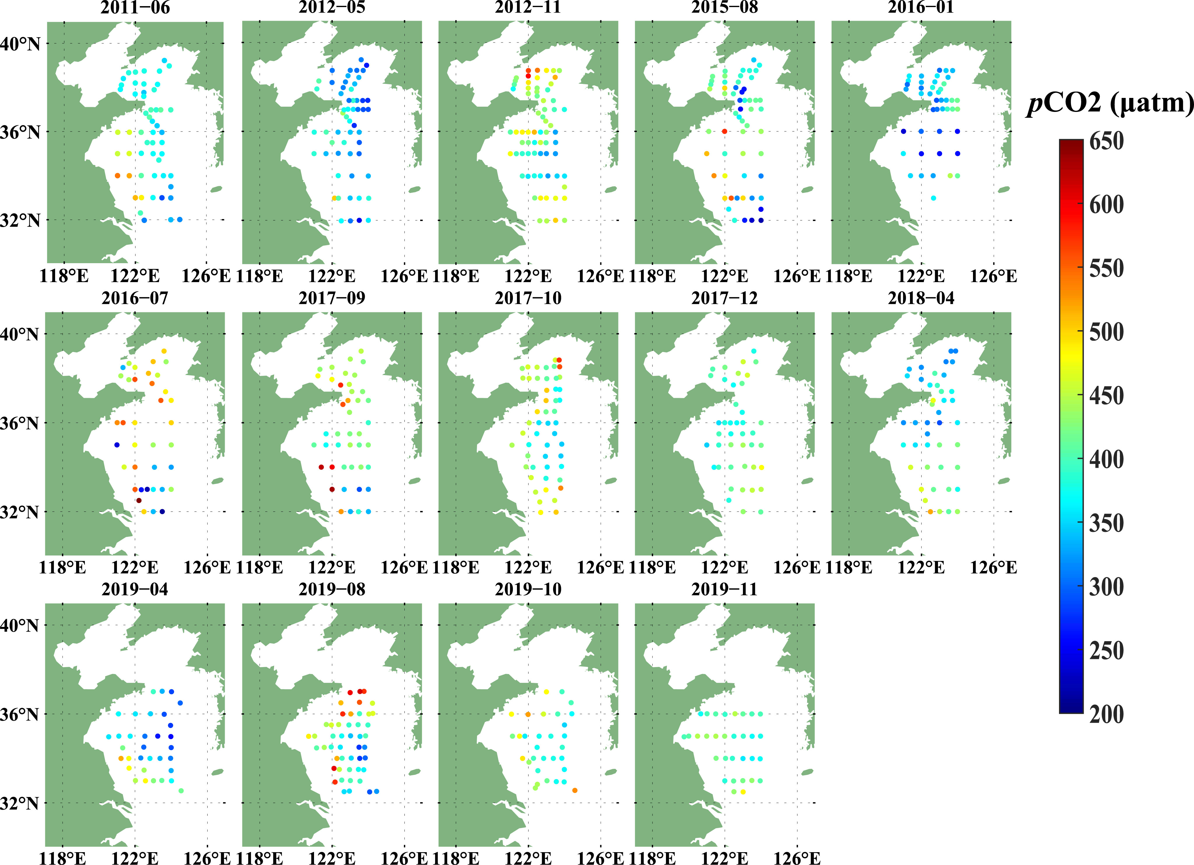
Figure 3 Spatial distribution of 638 matched pairs.

2.3 Model training and testing, and model selection

The 638 matched pairs were split into training and test data sets in a stratified random manner, where they accounted for 80% and 20% of the pairs, respectively. Histograms showing the distributions of the sample points in the training and test data sets are presented in Figure 4. Evaluation indicators comprising the RMSD, coefficient of determination (R²), mean absolute error (MAE), and mean absolute percentage error (MAPE) were employed to quantify the reliability of the pCO₂ model.

FIGURE 4

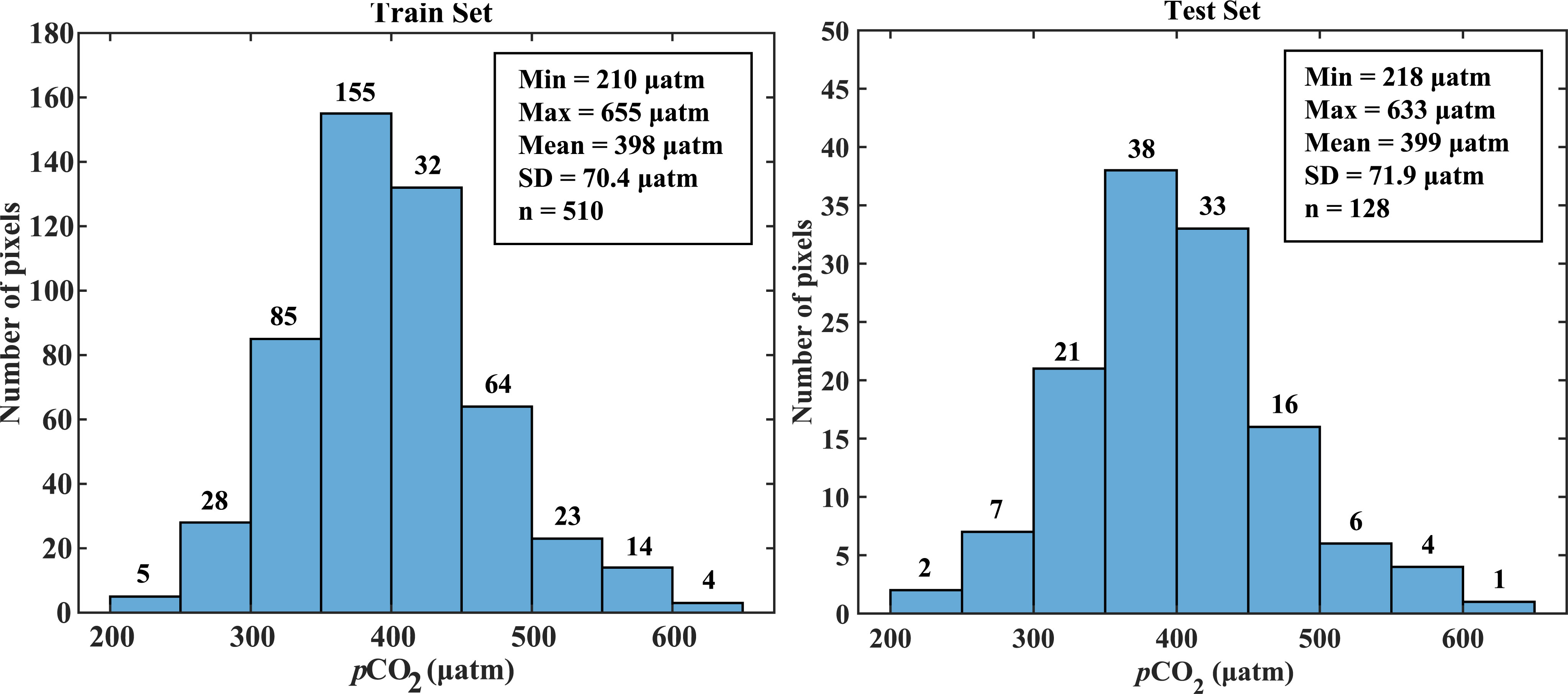
Figure 4 Histograms showing the distributions of the sample points in the training and test data sets.

Two machine learning algorithms comprising Random Forest (RF) and particle swarm optimization-support vector regression (PSO-SVR) were used to develop sea surface pCO₂ models because of their high generalizability for nonlinear relationships (Mountrakis et al., 2011). The inversion model was established using identical data sets. The algorithm was determined as formula (4).

$\begin{array}{ll}p{\text{CO}}_2=f(\text{input variables})=f(\text{SST},\text{Kd},\text{SSS},\text{Chl},\text{cos}(2\text{π}(\text{Julday}-\text{γ})/365)& (4)\end{array}$

The value of γ was optimized iteratively (0 to 365) until the RMSD reached a minimum value.

2.4 Random forest

The RF consists of multiple decision trees, where the structure of a single decision tree is based on a group of training data (Breiman, 2001). In RF, a bootstrap strategy is used to conduct resampling from the original data sets to produce multiple subgroups. The structure regression trees are then obtained for every subgroup, and the final output is the mean of the outputs of all regression trees.

RF model development (Figure 5) requires the determination of three customized parameters: the number of randomly selected variables for constructing the tree (mtry), the minimum number of terminal nodes for each tree (node size), and the number of trees (ntree) (Sun et al., 2016).

FIGURE 5

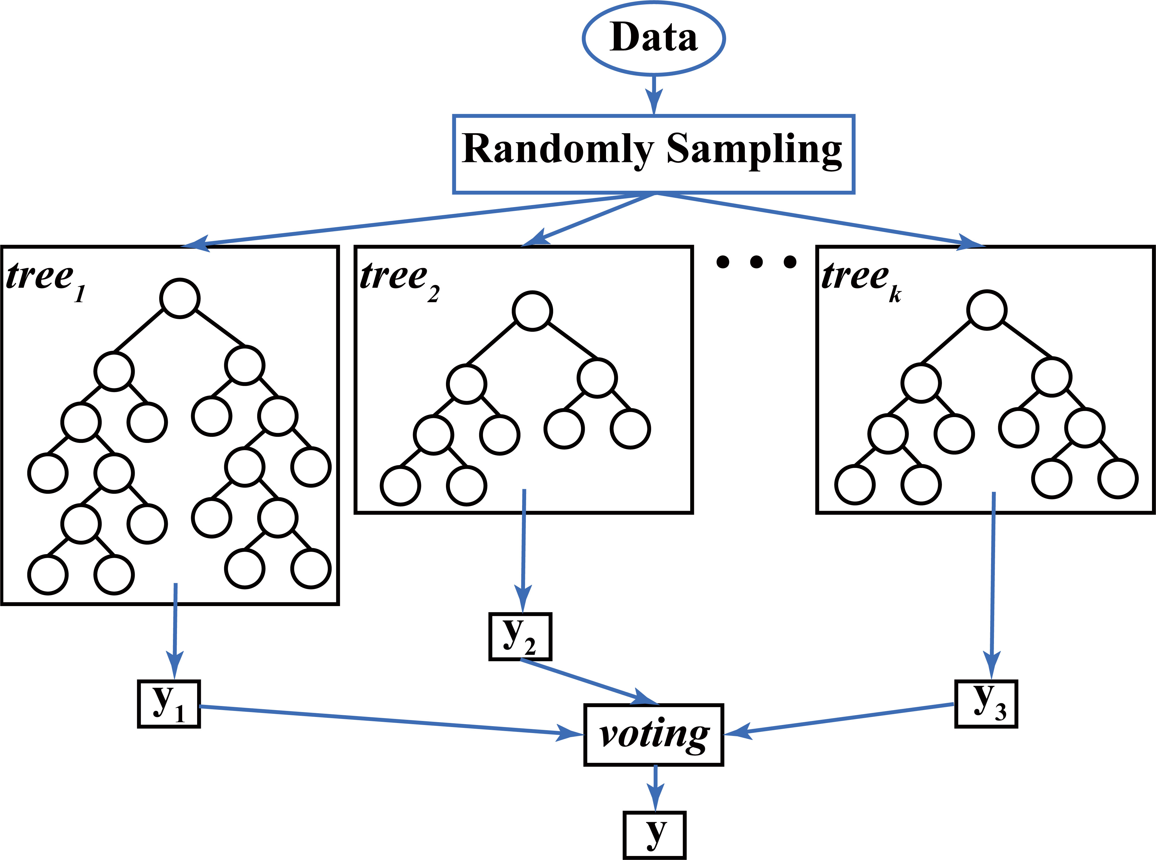
Figure 5 General Random Forest model development process.

The node size was set to 5 because this is a common value for regression models (Sun et al., 2016). The grid search method was used to determine the RF parameters ntree and mtry (Figure 6). The optimal values were determined with the minimal RMSD, and 4 and 200 were selected as the best mtry and ntree values, respectively, for the RF model.

FIGURE 6

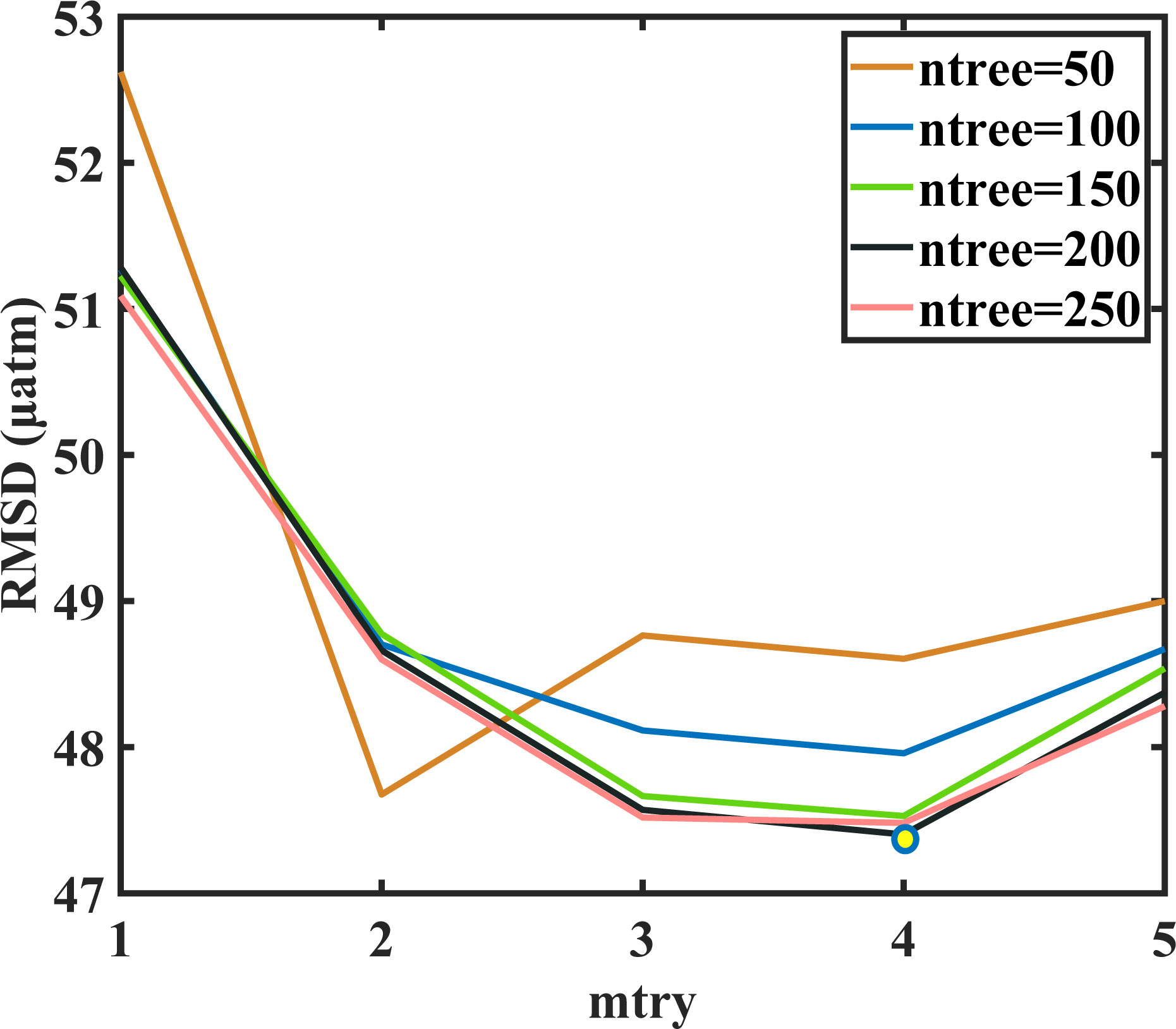
Figure 6 Influence of mtry and ntree on RMSD.

2.5 Model sensitivity to input variables

Sensitivity analysis was conducted to assess the sensitivity of the model to the inherent uncertainties in SST, SSS, Chl, and Kd. The original pCO₂ (using the original inputs) was compared with the new pCO₂ (using inputs with extra added uncertainties) derived from the same RF model to identify the model’s sensitivity to the uncertainty in these inputs. Only one input variable was changed in each analysis and the remaining variables were kept the same. Statistical parameters comprising the mean bias (MB), mean ratio (MR), RMSD, and R² were applied to quantify the sensitivity.

The uncertainties of environmental variables were determined by referring to published studies. In particular, the uncertainty of remote sensing SST is ≤ 1°C (Hao et al., 2017), the uncertainty of HYCOM SSS is about 0.5 when SSS is more than 32, the uncertainty of HYCOM SSS is about 3 when SSS is less than 32 (Jang et al., 2022), and the uncertainties of Chl and Kd are 32% and 48%, respectively (Cui et al., 2014). Thus, we used ± 1°C, ± 1, ± 30%, and ± 45% as the uncertainties of SST, SSS, Chl, and Kd, respectively.

3 Results

3.1 Model performance

Table 1 shows that RF outperformed PSO-SVR. The R² and RMSD values were 0.82 and 34 μatm, and 0.67 and 43 μatm for the model training and test data sets, respectively.

TABLE 1

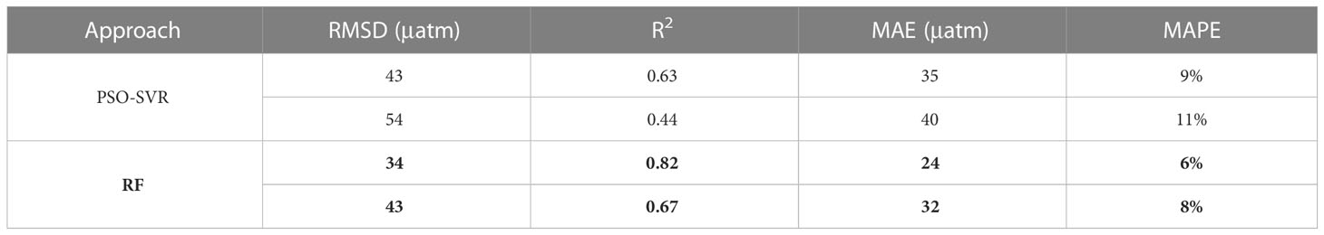
Table 1 Comparison of two empirical modeling approaches. .

The sea surface pCO₂ predicted by the RF model was slightly underestimated when the sea surface pCO₂ was larger than 500 μatm, and slightly overestimated when pCO₂ was smaller than 300 μatm (Figure 7). The pCO₂ values estimated by the model varied in the range of 250−550 μatm, with some larger than 550 μatm and lower than 250 μatm. A histogram showing the residuals (modeled pCO₂ minus field pCO₂) is presented in Figure 7, which demonstrates that 82.45% of the residuals were within the interval of ± 50, i.e., the observed 50 μatm pCO₂ standard deviation.

FIGURE 7

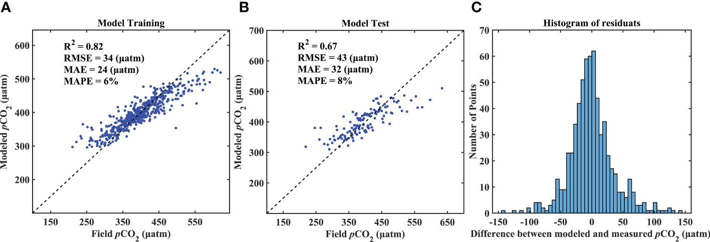
Figure 7 Performance evaluation for RF using (A) training and (B) test data sets; and (C) histogram of residuals.

3.2 Model sensitivity

Statistically, when a bias of +1°C was applied to the SST input, the RF model overestimated the sea surface pCO₂ slightly (RMSD = 10 μatm, R² = 0.96, MB = 3 μatm), and when a bias of –1°C was applied to the SST input, the RF model underestimated the sea surface pCO₂ slightly (R² = 0.96, RMSD = 10 μatm, MB = –2 μatm) (Figure 8). These results suggest that pCO₂ increased with SST, and vice versa, which is consistent with the relationship between temperature and pCO₂ in thermodynamics.

FIGURE 8

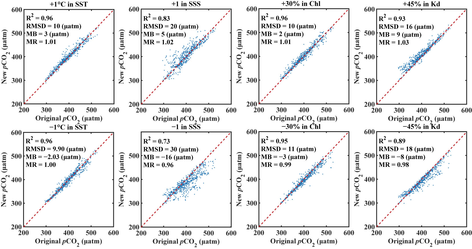
Figure 8 Sensitivity of RF model to the uncertainties in SST, SSS, Chl, and Kd.

Compared with the SST, the RF pCO₂ model was more sensitive to the uncertainties in SSS. Moreover, the RF model was more sensitive to lower SSS values, where a change of –1 in SSS resulted in a substantial decrease in the predicted pCO₂. In particular, with input +1 uncertainty in SSS, the RF pCO₂ model tended to overestimate the sea surface pCO₂ (R² = 0.83, RMSD = 20 μatm, and MB = 5 μatm) and with input –1 uncertainty in SSS, the RF pCO₂ model tended to greatly underestimate the sea surface pCO₂ (R² = 0.73, RMSD = 30 μatm, and MB = –16 μatm).

Similar to SST, the RF pCO₂ model exhibited minor sensitivity to Chl. When all data were used in the calculations with +30% uncertainties added, the RF model slightly overestimated pCO₂ (R² = 0.96, RMSD = 10 μatm, and MB = 2 μatm). With input –30% uncertainties in Chl, the RF model slightly underestimated pCO₂ (R² = 0.95, RMSD = 11 μatm, and MB = –3 μatm). Similarly, the RF pCO₂ model was insensitive to Kd. With +45% and –45% uncertainties added in Kd, the new pCO₂ was not very different from the original pCO₂. In particular, with a bias of +45% uncertainty added to Kd, the RF slightly overestimated the surface pCO₂ (R² = 0.93, RMSD = 16 μatm, and MB = 9 μatm), and with a bias of –45% uncertainty added, the RF pCO₂ model slightly underestimated the pCO₂ (R² = 0.89, RMSD = 18 μatm, and MB= –8 μatm).

The sensitivity of the RF model was different according to the uncertainty in each environment variable, but the differences introduced by each variable were generally within the range of the uncertainty of the model itself.

3.3 Seasonal and interannual variations in pCO₂ in the YS

The RF model was applied to monthly MODIS and HYCOM data for the period between January 2003 and December 2021 to generate monthly climatological maps and determine the annual trend in pCO₂ in the YS (Figure 9).

FIGURE 9

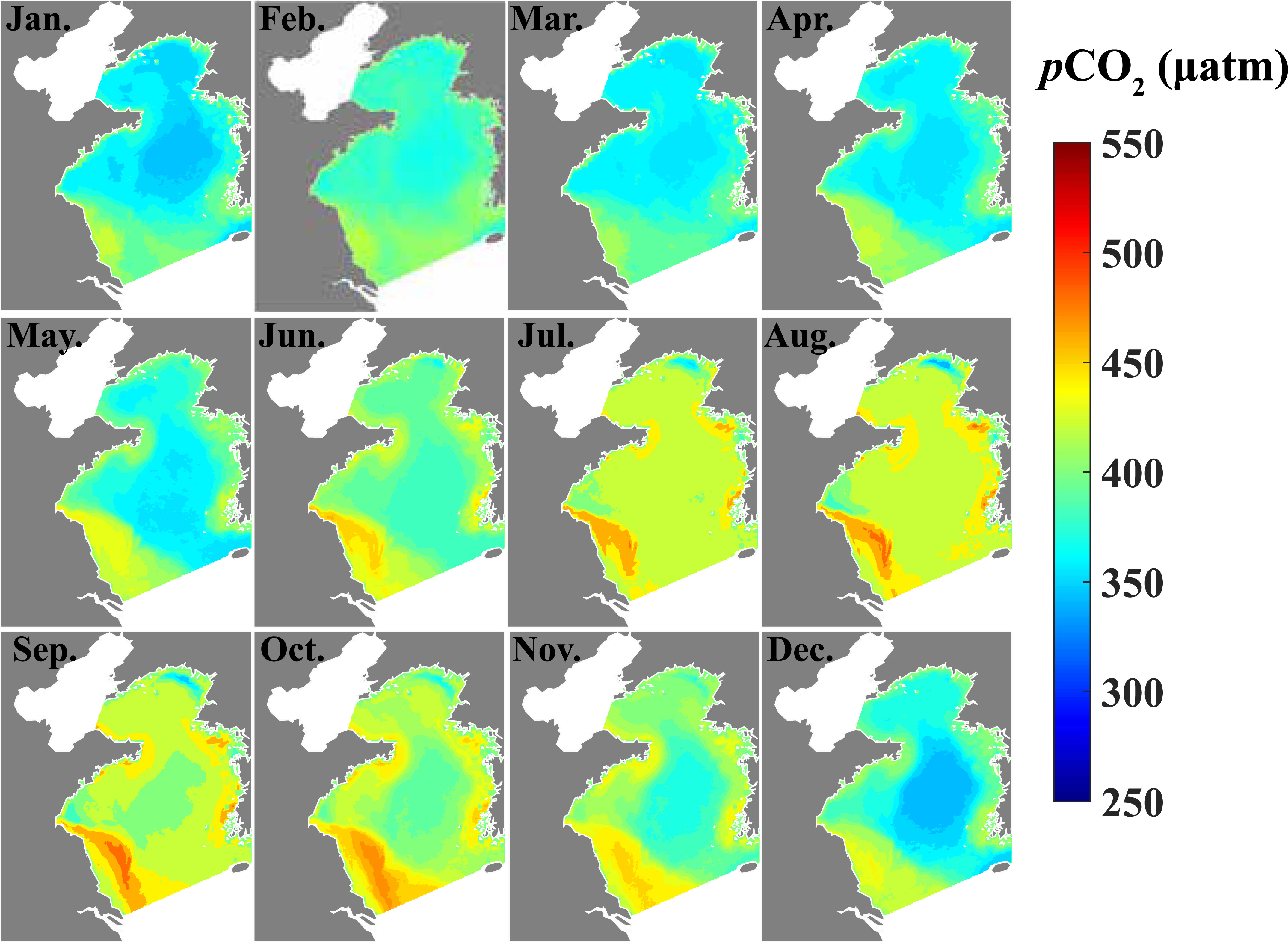
Figure 9 Monthly climatological maps of pCO₂ in the YS from January 2003 to December 2021.

Spatially, due to the effects of the hydrology environment and terrestrial organic matter, the pCO₂ values tended to decrease from the nearshore to central areas, and the highest pCO₂ values were observed in the SYS. Seasonally, there were apparent variations in pCO₂ throughout the YS (Figure 9). Statistically, the average sea surface pCO₂ values were 377 ± 7 μatm, 430 ± 6 μatm, 426 ± 11 μatm, and 378 ± 10 μatm in the spring, summer, autumn, and winter, respectively. In addition to these seasonal patterns, more complex variations were found in the spring and autumn (Figure S1). In most years, pCO₂ decreased in March because of phytoplankton blooms, and increased in September or November because of the collapsing seasonal stratification.

The annual mean sea surface pCO₂ values were extracted to explore the interannual variation. The results showed that the surface pCO₂ values in the YS increased between 2003 and 2021 at a rate of 0.36 μatm year⁻¹ (R² = 0.27, p< 0.05, N = 19) (Figure 10). According to the model sensitivity analysis results in section 3.2, when a bias of +1°C was applied to the SST input, the RF model overestimated pCO₂ by 10 μatm. The annual rate of change in the SST determined by the remote sensing products was 0.039°C year^–1 (Figure S2). Therefore, increasing the SST approximately led to an increase in the pCO₂ at a rate of 0.39 μatm year^–1 in the YS. The pCO₂ in the YS has increased in the past 19 years, but its rate of increase was lower than that for $pC{O}_2^{air}$ (with a rate of 2.31 μatm year⁻¹; R² = 0.99, p< 0.01, N = 19) in the same period (Figure S3). Therefore, the ΔpCO₂ (sea surface pCO₂– $pC{O}_2^{air}$) exhibited a remarkable decreasing trend with a rate of −1.95 μatm year⁻¹ (R² = 0.92, p< 0.01, N = 19).

FIGURE 10

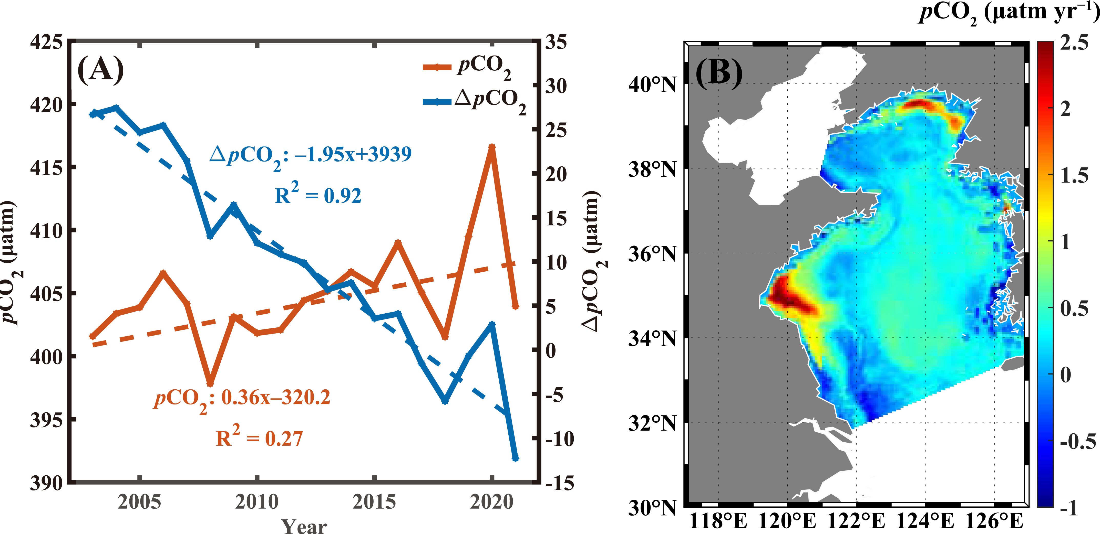
Figure 10 (A) Long-term trends in regional average pCO₂ and ΔpCO₂ (pCO₂ − $pC{O}_2^{air}$); and (B) spatial trends in pCO₂ during 2003–2021.

Moreover, the spatial trends in pCO₂ were obtained by calculating the trend for each grid in pCO₂ (Figure 10B). In general, pCO₂ increased in most regions of the YS, with a range from 0 to 2.78 μatm year⁻¹ from 2003 to 2021. Decreasing trends were also found in some regions. For example, pCO₂ decreased in the NYS and the runoff area of the Changjiang River. These results indicate that the NYS and runoff area of the Changjiang River have more substantial carbon absorption capacities. Both pCO₂ and Chl tended to decrease in the runoff area of the Changjiang River (Figures 10B, S4). Therefore, the decrease in the transportation of terrestrial organic matter might be the main reason for the decrease in pCO₂ in this area, which might alleviate the seasonal hypoxia phenomenon.

4 Discussion

4.1 Evaluation based on comparisons with field observations of sea surface pCO₂

Two algorithms were tested to establish models for estimating pCO₂. The best RMSD and R² values for the model were 43 μatm and 0.67 in the YS, respectively (Figure 7). The accuracy of four data sets were evaluated by comparing with field observations of sea surface pCO₂. The resolutions, names of the four data sets, and comparisons of the results are shown in Table 2.

TABLE 2

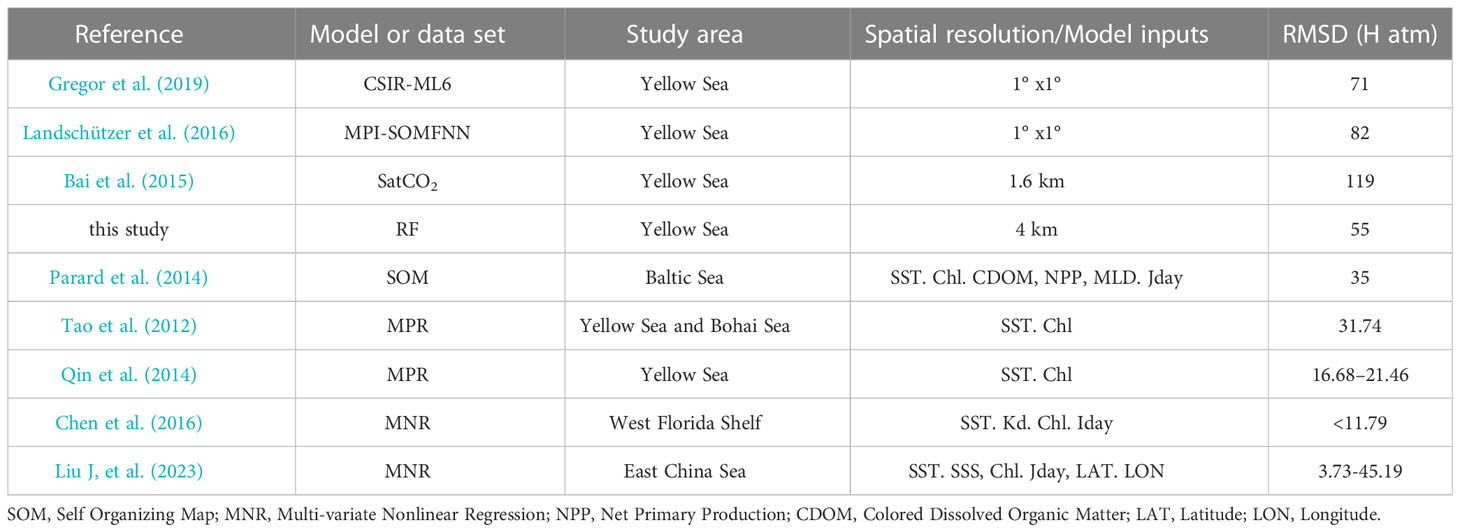
Table 2 Published models based on remote sensing of sea surface pCO₂ and global pCO₂ products.

Figure 11 shows scatter diagrams to compare the results. The pCO₂ derived from the RF model exhibited greater consistency (RMSD = 55 μatm) with the in-situ pCO₂ than CSIR-ML6 (RMSD = 71 μatm), MPI-SOMFNN (RMSD = 82 μatm), and SatCO₂ (RMSD = 119 μatm). The significant underestimation of the field pCO₂ by SatCO₂ was predictable because the algorithm was originally developed for the ECS and it may not be applicable to the YS. Significant differences between the global pCO₂ products and in-situ data in coastal seas were expected (Landschützer et al., 2020). Moreover, CSIR and ML6 were not effective at matching the pCO₂ in the YS, as shown by the number of scatter points in Figure 11. The comparison of four products showed that the RF model was the optimal method for estimating pCO₂ in the YS because the root mean square difference was less than those with the other three products (CSIR-ML6, MPI-SOMFNN, and SatCO₂). Understanding the variations in pCO₂ can provide greater insights into the response of the carbon absorption capacity to climate change in the YS. Erroneous estimates may be obtained in coastal seas if global pCO₂ products are used, which might affect quantification of the longer-term trends in global carbon budgets.

FIGURE 11

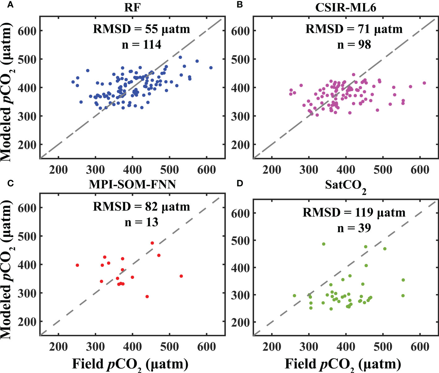
Figure 11 Scatter plots of pCO₂ obtained from (A) RF model, (B) CSIR-ML6, and (C) MPI-SOMFNN; and (D) SatCO₂ against the field pCO₂ in the test set.

4.2 Satellite estimation of pCO₂ in coastal seas

Due to its unique advantage in terms of high spatiotemporal resolution, satellite remote sensing is an effective method for observing the sea surface pCO₂. Table 2 lists some inversion models for pCO₂ in coastal seas. The maximum RMSD for these models was 45.19 μatm. Tao et al. (2012) and Qin et al. (2014) established pCO₂ estimation models based on MPR using the in-situ SST and Chl, and the RMSD values for the two models were 15.82−31.7 and 16.68–21.46, respectively, and both were less than 43. The error was small for the two models, mainly because the in-situ data used for modeling were mostly located in the YS center, with few data located in the nearshore area. The MPR-based inversion model was developed using the same training data sets employed in the present study, and the error was much larger than 43 μatm. Overall, the error was acceptable for the RF model developed in this study. The RMSD of the model for estimating the surface pCO₂ in the YS was higher than that in other marginal seas due to the following three reasons. (1) The uncertainty of satellite data and field pCO₂. In the YS, the error of satellite remote sensing Kd and Chl data can reach 48%, and 32%, respectively (Cui et al., 2014). Moreover, the pCO₂ data used in this study were converted from fCO₂, and fCO₂ was estimated using the dissolved inorganic carbon and total alkalinity. The uncertainty in the pCO₂ obtained by using this method is ± 5%, which is larger compared with ± 1% using directly measured pCO₂ data (Wang and Zhai, 2021). (2) The hydrological complexity of the YS environment leads to a wide range of sea surface pCO₂ changes. In particular, the magnitude of the change in pCO₂ in the YS is 450 μatm (Figure 3), but only about 350 μatm in the Gulf of Mexico (Fu et al., 2020) and the Gulf of Maine (Signorini et al., 2013). The performance of the model constructed for the YS was similar to that of a model for the Baltic Sea (RMSD = 47.48 μatm, R² = 0.63) (Zhang et al., 2021), where pCO₂ ranged from 100−600 μatm. (3) Importantly, the RF model needed to include all of the processes from 2011 to 2019. These three reasons explain why estimating pCO₂ is very difficult in the YS compared with other marginal seas, and thus the error is large.

4.3 Advantages and limitations of RF model

The comparisons of the models based on the two algorithms showed that the RF algorithm was advantageous for inverting the sea surface pCO₂ in the YS (Table 1; Figure 11), and the uncertainty was less than 50 μatm. However, the RF model still has some problems.

First, in the eastern YS, the seasonal variation in the pCO₂ obtained from the RF model differed compared with the in-situ pCO₂. Choi et al. (2019) found that pCO₂ tended to increase from May to February in the Southeastern YS. However, the maximum pCO₂ obtained by RF inversion was in August (Figure 9). Wang and Zhai (2021) divided the YS region west of 124°E into four regions and analyzed the seasonal variations in the pCO₂. They found that the maximum values in the four regions occurred in July, September, or October, with none in February. Due to the effect of hydrodynamics and other factors, the seasonal patterns in the pCO₂ differ greatly in the eastern YS and western YS. Therefore, the differences in the seasonal variations in pCO₂ may be explained by only using in-situ data for the area located west of 124°E for modeling, and thus the model was unable to fully identify the pCO₂ control process.

Second, using the RF model to compute the interannual trends in the pCO₂ could introduce uncertainties. The homogenously collected cruise data covered the whole annual period (Table 3). The variation in pCO₂ was influenced by physical and biogeochemical processes in the sea, and the increase in atmospheric CO₂ (Xue et al., 2016). However, the parameters (SST, Chl, Kd, and SSS) used in this study could only characterize the physical and biogeochemical processes in the sea. If changes in pCO₂ caused by increases in the atmospheric CO₂ could not be captured implicitly by one or more of the four parameters (SST, SSS, Chl, and Kd), uncertainties would be introduced when computing the interannual trend in the pCO₂ (Chen et al., 2019). The long-term trend of SST in the YS was influenced by regional climate change (Park et al., 2015), that is to say, the change of SST included the change of atmospheric CO₂ internally and implicitly, therefore, the increase in the SST appeared to can capture the effects of increasing atmospheric CO₂ on the pCO₂, the interannual trend was still credible to some extent.

TABLE 3

Table 3 Cruises and statistics for SST, SSS, and sea surface pCO₂ measurements used for model training and test (mean ± standard deviation).

Third, in the present study, RF performed poorly at simulating data from both ends of the data sets (underestimation for high values and overestimation for low values) (Figure 7), which may be explained as follows. First, due to the features of the algorithm itself, RF averages the results for all regression trees. The underestimation of extreme values and overestimation of small values appears to be a common problem for RF regression models (Čeh et al., 2018; Zimmerman et al., 2018; Wolfensberger et al., 2021). Second, the training data sets contained very few extreme pCO₂ values and they were underrepresented in the RF model, thereby leading to a more mean-biased output from the RF model.

In general, the problems with the RF model described above were caused by the unbalanced distributions of the modeling data sets. The number of extreme pCO₂ values (>550 μatm or<250 μatm) was relatively small in the field measurements (only 4.7%) but it did not seem to affect the interannual variation in the pCO₂. However, extreme pCO₂ is an influential component of the carbon cycle and it has significant impacts on the health of marine ecosystems. Therefore, it is very necessary to accurately estimate the extreme pCO₂. The crucial limitation of RF model is that its ability to estimate new pCO₂ is limited by the range of the training data set. That mean it can not estimate the pCO₂ beyond the range of the training data set (no extrapolation). Therefore, a better RF model may be developed by using a data set with a wider range of variation, which can improve the reproducibility of the RF model for extreme values. Therefore, we suggest that the modeling data set need to include all pCO₂ values that can be matched to the satellite data, some extreme values in the in-situ data sets should not be arbitrarily deleted (excluding the low and high values caused by measurement errors).

5 Conclusions

In this study, we constructed a RF model of the YS with SST, SSS, Chl, Kd, and Julday as the inputs. The RF model performed well at estimating pCO₂, with an RMSD of 43 μatm and R² of 0.67. The RF model was applied to satellite data from between 2003 and 2021 to obtain a 19-year time sequence of pCO₂ in the YS. Spatially, except for the eastern YS, the spatial pCO₂ distributions derived by the RF model matched with the in-situ data. According to the interannual changes, the sea surface pCO₂ increased in most regions of the YS, but there were differences among the regions, with decreased trends in the pCO₂ in the NYS and the runoff area of the Changjiang River, which appears to contrast with the background global warming and increasing atmospheric CO₂ concentration. The present study is the first to using machine learning methods to estimate the pCO₂, and also the first to determine the long-term trend in the pCO₂ in the YS. Future research should focus on obtaining balanced in-situ pCO₂ data and coupling the RF model with a mechanistic model to develop more accurate pCO₂ models. In addition, the reasons for the increasing trend in the pCO₂ in the YS should be explored.

Data availability statement

The original contributions presented in the study are included in the article/Supplementary Material. Further inquiries can be directed to the corresponding author.

Author contributions

WL: Methodology, Software, Writing-original draft. CL: Conceptualization, Resources, Writing-review & editing. WZ: Investigation, Writing-review & editing. HL: Software, Writing-review & editing. WM: Formal analysis. All authors contributed to the article and approved the submitted version.

Funding

This work was supported by the following research grants: the National Natural Science Foundation of China-Shandong joint fund (U1806203), Shandong Provincial Natural Science Foundation (ZR2020MD098), Shandong Universities Interdisciplinary Research and Innovation Team of Young Scholars (2020QNQT20).

Conflict of interest

The authors declare that the research was conducted in the absence of any commercial or financial relationships that could be construed as a potential conflict of interest.

Publisher’s note

All claims expressed in this article are solely those of the authors and do not necessarily represent those of their affiliated organizations, or those of the publisher, the editors and the reviewers. Any product that may be evaluated in this article, or claim that may be made by its manufacturer, is not guaranteed or endorsed by the publisher.

Supplementary material

The Supplementary Material for this article can be found online at: https://www.frontiersin.org/articles/10.3389/fmars.2023.1181095/full#supplementary-material

References

Bai Y., Cai W. J., He X. Q., Zhai W. D., Pan D. L., Dai M. H., et al. (2015). A mechanistic semi-analytical method for remotely sensing sea surface pCO₂ in river-dominated coastal oceans: a case study from the East China Sea. J. Geophys. Res. Ocean. 120, 2331–2349. doi: 10.1002/2014JC010632

CrossRef Full Text | Google Scholar

Breiman L. (2001). Random forests. Mach. Learn. 45, 5–32. doi: 10.1023/A:1010933404324

CrossRef Full Text | Google Scholar

Čeh M., Kilibarda M., Lisec A., Bajat B. (2018). Estimating the performance of random forest versus multiple regression for predicting prices of the apartments. ISPRS. Int. J. Geo-Inf. 7, 168. doi: 10.3390/ijgi7050168

CrossRef Full Text | Google Scholar

Chen S. L., Hu C. M., Barnes B. B., Wanninkhof R., Cai W. J., Barbero L., et al. (2019). A machine learning approach to estimate surface ocean pCO₂ from satellite measurements. Remote Sens. Environ. 228, 203–226. doi: 10.1016/j.rse.2019.04.019

CrossRef Full Text | Google Scholar

Chen S. L., Hu C. M., Byrne R. H., Robbins L. L., Yang B. (2016). Remote estimation of surface pCO₂ on the West Florida shelf. Cont. Shelf. Res. 128, 10–25. doi: 10.1016/j.csr.2016.09.004

CrossRef Full Text | Google Scholar

Chen S. L., Hu C. M., Cai W. J., Yang B. (2017). Estimating surface pCO₂ in the northern gulf of Mexico: which remote sensing model to use? Cont. Shelf. Res. 151, 94–110. doi: 10.1016/j.csr.2017.10.013

CrossRef Full Text | Google Scholar

Choi Y., Kim D., Cho S., Kim T. W. (2019). Southeastern yellow Sea as a sink for atmospheric carbon dioxide. Mar. pollut. Bull. 149, 110550. doi: 10.1016/j.marpolbul.2019.110550

PubMed Abstract | CrossRef Full Text | Google Scholar

Cui T. W., Zhang J., Tang J. W., Sathyendranath S., Groom S., Ma Y., et al. (2014). Assessment of satellite ocean color products of MERIS, MODIS and SeaWiFS along the East China coast (in the yellow Sea and East China Sea). ISPRS-J. Photogramm. Remote Sens. 87, 137–151. doi: 10.1016/j.isprsjprs.2013.10.013

CrossRef Full Text | Google Scholar

Dai M. H., Su J. Z., Zhao Y. Y., Hofmann E. E., Cao Z. M., Cai W. J., et al. (2022). Carbon fluxes in the coastal ocean: synthesis, boundary processes, and future trends. Annu. Rev. Earth Planet. Sci. 50, 593–626. doi: 10.1146/annurev-earth-032320-090746

CrossRef Full Text | Google Scholar

Deng X., Zhang G. L., Xin M., Liu C. Y., Cai W. J. (2021). Carbonate chemistry variability in the southern yellow Sea and East China Sea during spring of 2017 and summer of 2018. Sci. Total. Environ. 779, 146376. doi: 10.1016/j.scitotenv.2021.146376

PubMed Abstract | CrossRef Full Text | Google Scholar

Ding Y., Bao X. W., Yao Z. G., Song D. H., Song J., Gao J., et al. (2018). Effect of coastal-trapped waves on the synoptic variations of the yellow Sea warm current during winter. Cont. Shelf. Res. 167, 14–31. doi: 10.1016/j.csr.2018.08.003

CrossRef Full Text | Google Scholar

Friedlingstein P., Jones M. W., O’Sullivan M., Andrew R. M., Bakker D. C. E., Hauck J., et al. (2022). Global carbon budget 2021. Earth Syst. Sci. Data 14, 1917–2005. doi: 10.5194/essd-14-1917-2022

CrossRef Full Text | Google Scholar

Fu Z. Y., Hu L. S., Chen Z. D., Zhang F., Shi Z., Hu B. F., et al. (2020). Estimating spatial and temporal variation in ocean surface pCO₂ in the gulf of Mexico using remote sensing and machine learning techniques. Sci. Total. Environ. 745, 140965. doi: 10.1016/j.scitotenv.2020.140965

PubMed Abstract | CrossRef Full Text | Google Scholar

Gregor L., Lebehot A. D., Kok S., Scheel Monteiro P. M. (2019). A comparative assessment of the uncertainties of global surface ocean CO₂ estimates using a machine-learning ensemble (CSIR-ML6 version 2019a) – have we hit the wall? Geosci. Model. Dev. 12, 5113–5136. doi: 10.5194/gmd-12-5113-2019

CrossRef Full Text | Google Scholar

Gu Y. Y., Katul G. G., Cassar N. (2021). The intensifying role of high wind speeds on air-sea carbon dioxide exchange. Geophys. Res. Lett. 48, e2020GL090713. doi: 10.1029/2020GL090713

CrossRef Full Text | Google Scholar

Hales B., Strutton P. G., Saraceno M., Letelier R., Takahashi T., Feely R., et al. (2012). Satellite-based prediction of pCO₂ in coastal waters of the eastern north pacific. Prog. Oceanogr. 103, 1–15. doi: 10.1016/j.pocean.2012.03.001

CrossRef Full Text | Google Scholar

Hao Y. L., Cui T. W., Singh V. P., Zhang J., Yu R. H., Zhang Z. L. (2017). Validation of MODIS Sea surface temperature product in the coastal waters of the yellow Sea. IEEE J. Sel. Top. Appl. Earth Observ. Remote Sens. 10, 1667–1680. doi: 10.1109/JSTARS.2017.2651951

CrossRef Full Text | Google Scholar

Jang E., Kim Y. J., Im J., Park Y.-G., Sung T. (2022). Global sea surface salinity via the synergistic use of SMAP satellite and HYCOM data based on machine learning. Remote Sens. Environ. 273, 112980. doi: 10.1016/j.rse.2022.112980

CrossRef Full Text | Google Scholar

Landschützer P., Gruber N., Bakker D. C. (2016). Decadal variations and trends of the global ocean carbon sink. Glob. Biogeochem. Cycle 30, 1396–1417. doi: 10.1002/2015GB005359

CrossRef Full Text | Google Scholar

Landschützer P., Gruber N., Bakker D. C. E., Schuster U. (2014). Recent variability of the global ocean carbon sink. Glob. Biogeochem. Cycle 28, 927–949. doi: 10.1002/2014GB004853

CrossRef Full Text | Google Scholar

Landschützer P., Gruber N., Bakker D. C. E., Stemmler I., Six K. D. (2018). Strengthening seasonal marine CO₂ variations due to increasing atmospheric CO₂ nature climate change. Nat. Clim. Chang. 8, 146–150. doi: 10.1038/s41558-017-0057-x

CrossRef Full Text | Google Scholar

Landschützer P., Laruelle G. G., Roobaert A., Regnier P. (2020). A uniform pCO₂ climatology combining open and coastal oceans. Earth Syst. Sci. Data 12, 2537–2553. doi: 10.5194/essd-12-2537-2020

CrossRef Full Text | Google Scholar

Laruelle G. G., Cai W. J., Hu X. P., Gruber N., Mackenzie F. T., Regnier P. (2018). Continental shelves as a variable but increasing global sink for atmospheric carbon dioxide. Nat. Commun. 9, 1–11. doi: 10.1038/s41467-017-02738-z

PubMed Abstract | CrossRef Full Text | Google Scholar

Le C. F., Gao Y. Y., Cai W. J., Lehrter J. C., Bai Y., Jiang Z. P. (2019). Estimating summer sea surface pCO₂ on a river-dominated continental shelf using a satellite-based semi-mechanistic model. Remote Sens. Environ. 225, 115–126. doi: 10.1016/j.rse.2019.02.023

CrossRef Full Text | Google Scholar

Lefevre N., Watson A. J., Watson A. R. (2005). A comparison of multiple regression and neural network techniques for mapping in situ pCO₂ data. Tellus. Ser. B-Chem. Phys. Meteorol. 57, 375–384. doi: 10.3402/tellusb.v57i5.16565

CrossRef Full Text | Google Scholar

Li C. L., Zhai W. D. (2019). Decomposing monthly declines in subsurface-water pH and aragonite saturation state from spring to autumn in the north yellow Sea. Cont. Shelf. Res. 185, 37–50. doi: 10.1016/j.csr.2018.11.003

CrossRef Full Text | Google Scholar

Liu J., Bellerby R. G., Zhu Q., Ge J. Z. (2023). Estimation of sea surface pCO₂ and air–sea CO₂ flux in the East China Sea using in-situ and satellite data over the period 2000–2016. Cont. Shelf. Res. 254, 104879. doi: 10.1016/j.csr.2022.104879

CrossRef Full Text | Google Scholar

Liu Q., Dong X., Chen J. S., Guo X. H., Zhang Z. R., Xu Y., et al. (2019). Diurnal to interannual variability of sea surface pCO₂ and its controls in a turbid tidal-driven nearshore system in the vicinity of the East China Sea based on buoy observations. Mar. Chem. 216, 103690. doi: 10.1016/j.marchem.2019.103690

CrossRef Full Text | Google Scholar

Liu S. C., Luo Z. P., Wang Y. W., Rao Q. R., Zhang X. S., Yu B., et al. (2023). Interannual variation in winter thermal front to the east of the Shandong peninsula in the yellow Sea. J. Sea. Res. 193, 102370. doi: 10.1016/j.seares.2023.102370

CrossRef Full Text | Google Scholar

Liu Z. Y., Wei H., Lozovatsky I., Fernando H. (2009). Late summer stratification, internal waves, and turbulence in the yellow Sea. J. Mar. Syst. 77, 459–472. doi: 10.1016/j.jmarsys.2008.11.001

CrossRef Full Text | Google Scholar

Liu J. L., Xia J., Zhuang M. M., Zhang J. H., Sun Y. Q., Tong Y. C., et al. (2021). Golden seaweed tides accumulated in pyropia aquaculture areas are becoming a normal phenomenon in the yellow Sea of China. Sci. Total. Environ. 774, 145726. doi: 10.1016/j.scitotenv.2021.145726

CrossRef Full Text | Google Scholar

Lohrenz S. E., Cai W. J., Chen F. Z., Chen X. G., Tuel M. (2010). Seasonal variability in air-sea fluxes of CO₂ in a river-influenced coastal margin. J. Geophys. Res. Ocean. 115 (C10). doi: 10.1029/2009jc005608

CrossRef Full Text | Google Scholar

Lu X. L., Liu C. L., Niu Y., Yu S. X. (2021). Long-term and regional variability of phytoplankton biomass and its physical oceanographic parameters in the yellow Sea, China. Estuar. Coast. Shelf. Sci. 260, 107497. doi: 10.1016/j.ecss.2021.107497

CrossRef Full Text | Google Scholar

Mignot A., von Schuckmann K., Landschützer P., Gasparin F., van Gennip S., Perruche C., et al. (2022). Decrease in air-sea CO₂ fluxes caused by persistent marine heatwaves. Nat. Commun. 13, 4300. doi: 10.1038/s41467-022-31983-0

PubMed Abstract | CrossRef Full Text | Google Scholar

Mountrakis G., Im J., Ogole C. (2011). Support vector machines in remote sensing: a review. ISPRS-J. Photogramm. Remote Sens. 66, 247–259. doi: 10.1016/j.isprsjprs.2010.11.001

CrossRef Full Text | Google Scholar

Parard G., Charantonis A., Rutgerson A. (2014). Remote sensing algorithm for sea surface CO₂ in the Baltic Sea. Biogeosci. Discuss. 11, 12255–12294. doi: 10.5194/bgd-11-12255-2014

CrossRef Full Text | Google Scholar

Park K.-A., Lee E.-Y., Chang E., Hong S. (2015). Spatial and temporal variability of sea surface temperature and warming trends in the yellow Sea. J. Mar. Syst. 143, 24–38. doi: 10.1016/j.jmarsys.2014.10.013

CrossRef Full Text | Google Scholar

Qin B. Y., Tao Z., Li Z. W., Yang X. F. (2014). Seasonal changes and controlling factors of sea surface pCO₂ in the yellow Sea. IOP. Conf. Ser.: Earth Environ. Sci. 17, 012025. doi: 10.1088/1755–1315/17/1/012025

CrossRef Full Text | Google Scholar

Qu B. X., Song J. M., Yuan H. M., Li X. G., Li N. (2014). Air-sea CO₂ exchange process in the southern yellow Sea in April of 2011, and June, July, October of 2012. Cont. Shelf. Res. 80, 8–19. doi: 10.1016/j.csr.2014.02.001

CrossRef Full Text | Google Scholar

Rödenbeck C., Keeling R. F., Bakker D. C., Metzl N., Olsen A., Sabine C., et al. (2013). Global surface-ocean pCO₂ and sea–air CO₂ flux variability from an observation-driven ocean mixed-layer scheme. Ocean. Sci. 9, 193–216. doi: 10.5194/os-9-193-2013

CrossRef Full Text | Google Scholar

Signorini S. R., Mannino A., Najjar R. G. Jr., Friedrichs M. A. M., Cai W. J., Salisbury J., et al. (2013). Surface ocean pCO₂ seasonality and sea-air CO₂ flux estimates for the north American east coast. J. Geophys. Res. Ocean. 118, 5439–5460. doi: 10.1002/jgrc.20369

CrossRef Full Text | Google Scholar

Sun H. W., Gui D. W., Yan B. W., Liu Y., Liao W. H., Zhu Y., et al. (2016). Assessing the potential of random forest method for estimating solar radiation using air pollution index. Energy Conv. Manage. 119, 121–129. doi: 10.1016/j.enconman.2016.04.051

CrossRef Full Text | Google Scholar

Tao Z., Qin B. Y., Li Z. W., Yang X. F. (2012). Satellite observations of the partial pressure of carbon dioxide in the surface water of the huanghai Sea and the bohai Sea. Acta Oceanol. Sin. 31, 67–73. doi: 10.1007/s13131-012-0207-y

CrossRef Full Text | Google Scholar

Wang S. Y., Zhai W. D. (2021). Regional differences in seasonal variation of air–sea CO₂ exchange in the yellow Sea. Cont. Shelf. Res. 218, 104393. doi: 10.1016/j.csr.2021.104393

CrossRef Full Text | Google Scholar

Wolfensberger D., Gabella M., Boscacci M., Germann U., Berne A. (2021). RainForest: a random forest algorithm for quantitative precipitation estimation over Switzerland. Atmospheric. Measurement. Techniques. 14, 3169–3193. doi: 10.5194/amt-14-3169-2021

CrossRef Full Text | Google Scholar

Xiong T. Q., Wei Q. S., Zhai W. D., Li C. L., Wang S. Y., Zhang Y. X., et al. (2020). Comparing subsurface seasonal deoxygenation and acidification in the yellow Sea and northern East China Sea along the north-to-South latitude gradient. Front. Mar. Sci. 7, 686. doi: 10.3389/fmars.2020.00686

CrossRef Full Text | Google Scholar

Xue L., Cai W. J., Hu X. P., Sabine C., Jones S., Sutton A. J., et al. (2016). Sea Surface carbon dioxide at the Georgia time series site, (2006–2007): air–sea flux and controlling processes. Prog. Oceanogr. 140, 14–26. doi: 10.1016/j.pocean.2015.09.008

CrossRef Full Text | Google Scholar

Xue L., Zhang L., Cai W.-J., Jiang L.-Q. (2011). Air-sea CO2 fluxes in the southern yellow Sea: an examination of the continental shelf pump hypothesis. Cont. Shelf. Res. 31, 1904–1914. doi: 10.1016/j.csr.2011.09.002

CrossRef Full Text | Google Scholar

Ye H. J., Tang S. L., Morozov E. (2022). Variability in Sea surface pCO₂ and controlling factors in the bay of Bengal based on buoy observations at 15°N, 90°E. J. Geophys. Res. Ocean. 127, e2022JC018477. doi: 10.1029/2022JC018477

CrossRef Full Text | Google Scholar

Yu S. Q., Xiong T. Q., Zhai W. D. (2022). Quasi-synchronous accumulation of apparent oxygen utilization and inorganic carbon in the south yellow Sea cold water mass from spring to autumn: the acidification effect and roles of community metabolic processes, water mixing and spring thermal state. Front. Mar. Sci. 9, 858871. doi: 10.3389/fmars.2022.858871

CrossRef Full Text | Google Scholar

Zhai W. D. (2018). Exploring seasonal acidification in the yellow Sea. Sci. China Earth Sci. 61, 647–658. doi: 10.1007/s11430-017-9151-4

CrossRef Full Text | Google Scholar

Zhai W. D., Zheng N., Huo C., Xu Y., Zhao H. D., Li Y. W., et al. (2014). Subsurface pH and carbonate saturation state of aragonite on the Chinese side of the north yellow Sea: seasonal variations and controls. Biogeosciences 11, 1103–1123. doi: 10.5194/bg-11-1103-2014

CrossRef Full Text | Google Scholar

Zhang S. P., Rutgersson A., Philipson P., Wallin M. B. (2021). Remote sensing supported Sea surface pCO₂ estimation and variable analysis in the Baltic Sea. Remote Sens. 13, 259. doi: 10.3390/rs13020259

CrossRef Full Text | Google Scholar

Zimmerman N., Presto A. A., Kumar S. P., Gu J., Hauryliuk A., Robinson E. S., et al. (2018). A machine learning calibration model using random forests to improve sensor performance for lower-cost air quality monitoring. Atmos. Meas. Tech. 11, 291–313. doi: 10.5194/amt-11-291-2018

CrossRef Full Text | Google Scholar