A demographic model to forecast Dinophysis acuminata harmful algal blooms

1 Introduction

Harmful algal bloom (HAB) is an international term adopted by the Intergovernmental Oceanographic Commission (ICO) of the United Nations Educational, Scientific and Cultural Organization (UNESCO) to refer to any proliferation of microalgae (regardless of the density) perceived as harmful owing to its negative impact on public health, aquaculture, the environment and/or recreational activities (Kudela et al., 2015; Reguera et al., 2016; FAO, 2023). HABs constitute a serious threat to public health as well as sustainable coastal and marine development worldwide. HABs cannot easily be eliminated or prevented, but the potentially negative consequences can be managed and mitigated (FAO, 2023). Adopting an adequate suit of actions in due time is particularly relevant for aquaculture production systems. Among the most problematic HAB events are those associated with proliferations of Dinophysis species, mainly D. acuminata and D. acuta, which, even at low cell densities, cause Diarrheic Shellfish Poisoning (DSP) events. These marine mixotrophic dinoflagellates are producers of different analogues of the okadaic acid group of toxins and the main cause of shellfish harvesting closures in boundary upwelling systems (Trainer et al., 2010) as in the eastern Atlantic coasts of Europe (Reguera et al., 2014; Swan et al., 2018), particularly in the Iberian Peninsula (Vale et al., 2008; Fernández et al., 2019). Here, D. acuminata is the dominant species and it blooms (10² – 10⁴ cells·L^-1) mainly from April to October, coinciding with the upwelling season. Environmental factors are known to shape the proliferation and distribution of Dinophysis species (Díaz et al., 2013, 2016; Fernández et al., 2019; Lima et al., 2022). As a consequence, considerable effort has been devoted to understanding the ecophysiology, population dynamics and bloom development of D. acuminata over the past two decades (Smayda, 1997; Anschütz et al., 2022; Lima et al., 2022; FAO, 2023).

The development of sustainable shellfish aquaculture is highly dependent on the provision of reliable monitoring and predictive information on the occurrence of HABs. To assist the day-to-day management activities, it is fundamental to disclose regular information on HAB and biotoxins risk to end-users. Around the world, HAB alert bulletins and warning systems vary in complexity and can be delivered by a range of platforms using traditional environmental data or based on purely computational methods (Anderson et al., 2015; Lima et al., 2022; Wang et al., 2022; FAO, 2023). Reports rely on field observations, ocean colour satellite imagery, models, historical trends, public health reports, buoy data and forecasts of potential bloom progression (e.g. bulletins from NOAA, EUA; Marine Institute, Ireland; INTECMAR, Galicia; IPMA, Portugal). Multiple methods exist for monitoring algal densities and signalling the presence of algal blooms (Anderson, 2009; Stumpf et al., 2009, 2010, FAO, 2023). In situ species-specific cell counts have the highest confidence but the spatial and temporal resolution of the sampling is generally limited. In this regard, the Portuguese Institute for Sea and Atmosphere (IPMA), which is the national government agency responsible for shellfish toxicity monitoring, uses two thresholds of Dinophysis cell density: 200 cells·L^-1 to publicly emit a HAB warning alert and 500 cells·L^-1 to propose a DSP precautionary closure of shellfish harvesting.

Remote sensing has the advantage of providing large spatial coverage and with finer resolutions, although temporal frequency can be limited by clouds. Remote sensing of the coastal ocean is intricate. Satellite imagery of coastal and inland waters require atmospheric correction algorithms (Zhang et al., 2014; Fan et al., 2017; Lu et al., 2018; Ilori et al., 2019). Near-coast processes as daily winds, river run-off or coastal upwelling can also bias data from satellite imagery, especially due to their impact on ocean colour and plankton assemblages, and the high spatial and temporal resolutions of their dynamics (Shen et al., 2012; Smith and Bernard, 2020). Operational models allow near real-time forecasting and can be used to calculate the temporal and spatial coverage of phytoplankton distribution and chlorophyll-a. Data sampling schemes (spatial and temporal) have great influence on the accuracy of the forecasts (Stumpf et al., 2009, 2010).

In this work, we propose a demographic model of D. acuminata as a tool for forecasting its blooms and help decision making. The model is applied separately to distinct regions of the Portuguese coast with the goals of anticipating two operational thresholds concentration of 200 and 500 cells·L^-1. For that, we assess the set of environmental variables governing D. acuminata growth.

2 Materials and methods

The study was conducted along the Portuguese continental coast, which together with Galicia, comprise the west coast of Iberia, constituting the northern limit of the northeast Atlantic upwelling system (Figure 1) (Ambar and Dias, 2008; Alvarez et al., 2010). Usually, upwelling occurs from late Spring to early Autumn. Along the western coast, it is driven by northerly winds, while along the southern margin, although not as frequent or intense, these events are mainly due to westerly winds. During upwelling, the shelf circulation is characterized by alongshore flows roughly aligned with the wind direction. This means that during the summer months, the water transport is mainly southward and eastward, respectively, along the west and south coasts of the study area. During winter the winds relax, with intermittent periods of both upwelling- and downwelling-favourable winds (Ambar and Dias, 2008; Alvarez et al., 2010; Leitão et al., 2019), inducing local inversion in coastal shelf currents.

Figure 1

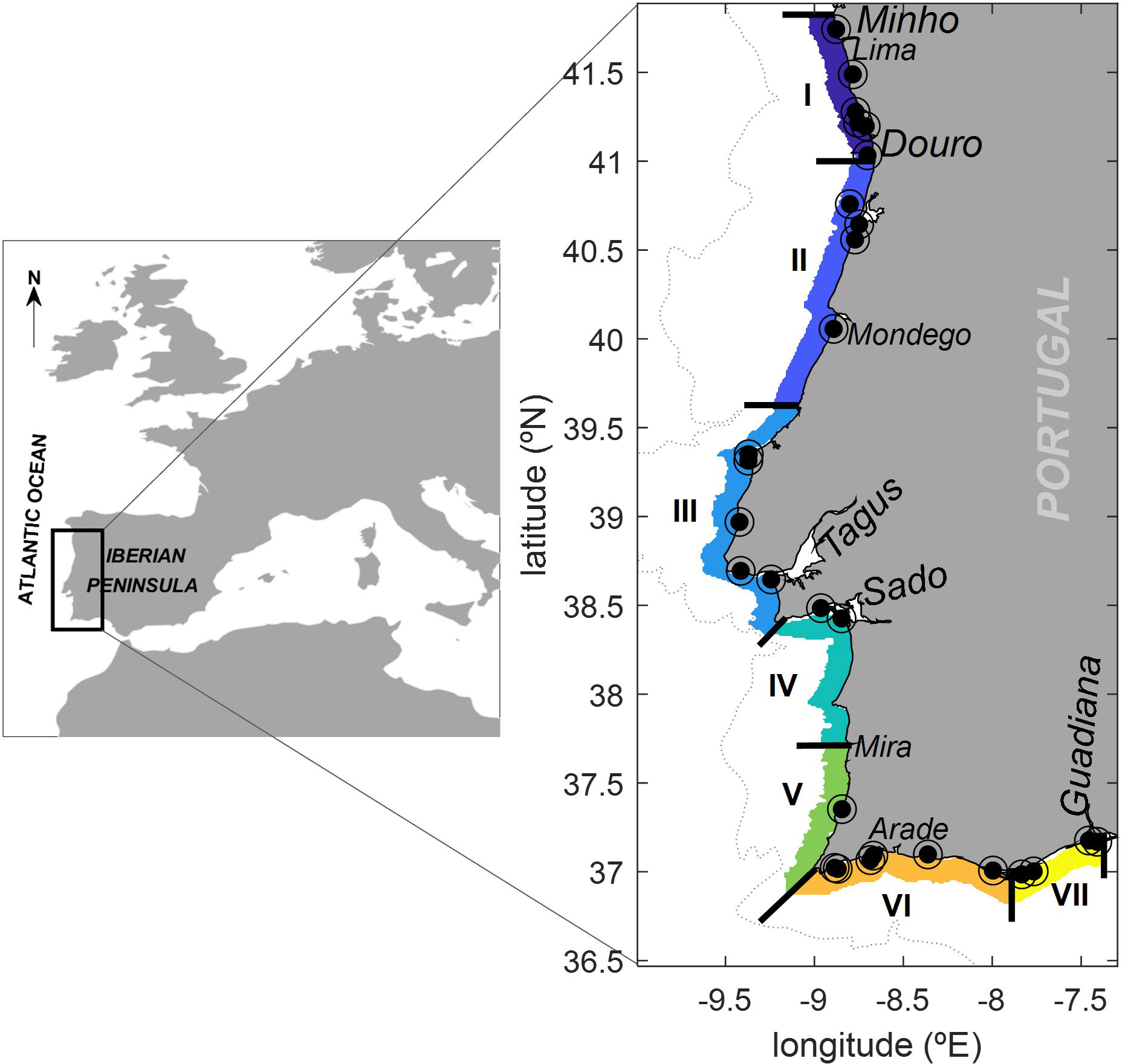
Figure 1 Map of the study area (Portuguese coast). Names indicate the location of estuaries of the main rivers flowing into the shelf. ◉ - Phytoplancton sampling stations. Roman numbers I to VII indicate the 7 regions/zones studied.

The thickness of the upper ocean mixed layer and seasonal thermocline, also varies widely according to the season: in winter, vertical stratification is low, with homogeneous mixed layer depths (MLD) reaching about 200 meters, while during the summer upwelling season, the water column is highly stratified, with MLD typically narrower than 20 meters.

The coastal area studied is also under the influence of several rivers, where fresh water run-offs also impact the inner shore stratification pattern (Cunha, 2001). The main rivers flowing into the shelf are highlighted in Figure 1. Along the western margin, among all the rivers depicted in this figure, the Minho, Douro, Tagus, and Sado rivers stand out as a the most significant freshwater sources to the shelf, while on the southern coast, the Guadiana detaches as the most important one. This fresh-water outflows, can generate lenses of low buoyancy water that can spread offshore, with variable seasonal distances, occasionally exhibiting a persistent signature throughout the year. This is the case of the Western Iberia Buoyant Plume (WIBP), first identified by Peliz et al. (2002), which extends meridionally from approximately 40°N, to the Galician coast, in the northern region of the study area. It results from the outflow of several regional rivers, from which the Minho and Douro are the main contributors (Otero et al., 2008). The WIBP maintains a year-round presence in the area and significantly impacts both the structure of upwelling and the expected vertical stratification pattern along the inner shelf.

2.1 Data collection

The monitoring of D. acuminata cell density in the seawater has been implemented by the National Monitoring System of Molluscs for human consumption safety, held by the Portuguese Institute for Sea and Atmosphere (IPMA). The sampling stations are located in known plankton retention/accumulation areas and/or in shellfish production areas (see Figure 1). The time series of D. acuminata cell density analysed in this study comprised 13 years of water samples taken on a weekly basis, from the 1^st of January of 2006 until the 31^st of December of 2018. However, it was not possible to implement a strict protocol of 7 day census intervals. Due to logistics constrains, in some cases the census intervals were smaller (6 days) or larger (up to 11 days). Water samples were collected during high tide and field preserved in 1% neutral Lugol’s iodine solution. The Utermohl (1958) method was applied with the sedimentation of 50 ml water samples that, within 48h were analysed for the presence of D. acuminata, as described in the IOC list (Lundholm et al., 2009), under inverted microscopy at a magnification of 200x. Abundances were expressed in cells·L⁻¹, with a method detection limit of 20 cells·L^-1.

The environmental variables tested as predictors of D. acuminata growth were sea surface temperature (SST), salinity, Chlorophyll-a, upwelling Bakun index, ocean mix layer depth (defined by sigma theta), photosynthetically active radiation (PAR), wave height and precipitation. Satellite imagery, modelling and in situ information were used to construct time series of these variables with spatial and temporal resolutions adjusted to that of the D. acuminata sampling. The upwelling Bakun index and precipitation data were retrieved in situ by IPMA. The SST, salinity and Chlorophyl-a data were retrieved from satellite imagery provided by the Copernicus Marine Environment Monitoring Service (available at http://marine.copernicus.eu/). The ocean mixed layer depth was retrieved from numerical model re-analyses provided by the Copernicus Marine Environment Monitoring Service. The PAR and wave height data were retrieved from numerical model re-analyses provided by the European Centre for Medium Weather Forecast (ERA-Interim reanalysis atmospheric products available at https://www.ecmwf.int).

2.2 Modelling

The Portuguese HAB species monitoring program started in 1998 and, based on that time series of data, IPMA operates a spatial sub-division of the coast into seven regions (see Figure 1). The environmental variables were aggregated according to those seven regions by averaging. The environmental variables were initially obtained with a time resolution of hours, up to a maximum of 1 day. As such, temporal composites were calculated to facilitate comparison with the D. acuminata data. Depending on the environmental variable, either an average or sum-based rule was applied. Various temporal solutions were experimented with, including averages over the preceding 3-day, 5-day, and 7-day periods. The growth of D. acuminata exhibited a stronger correlation with the 5-day averages of environmental variables. Subsequently, the analysis was conducted using these 5-day averages.

Biological populations typically grow following sigmoid-shaped functions (Gompertz, 1825; Winsor, 1932; Weibull, 1951; Paine et al., 2012). The sigmoid growth of D. acuminata in each of these zones was modelled following the same protocol as in Vieira et al. (2018, 2021, 2022). The population growth corresponded to the traditional n_t+Δt =R×n_t, where n is population density (in cell·L^-1), R is the growth rate and t is the time instance. Because time intervals (Δt) between consecutive census varied from 7 to 11 days, parameter estimation for this non-linear growth required adaptation. In this case, n was transformed to x=log₁₀(n), enabling the growth rate to be estimated as log₁₀R=Δx. The model becomes n_t+Δt =10^x+Δx. Then, to standardized for unit time, the model coefficients were estimated from linear regression of Δx/Δt on x so that Δx/Δt = a+b·x (Figure 2). Consequently, the model became n_t+Δt =10^{x+(a+b·x)Δt}. The y-axis intercept (a) corresponded to the maximum exponential growth verified when the population size was small. The negative sign of parameter b led to a line with negative slope corresponding to growth rate de-acceleration as the population got larger. The x-axis intercept (given by -a/b) corresponded to the largest possible population size beyond which growth was unsustainable; commonly referred in the specialized literature as the “Carrying Capacity” or “K”. This way, a population will reach the carrying capacity allowed by specific environmental conditions given time enough. If the conditions are good the carrying capacity will be large. When conditions worsen the population is momentarily above the new carrying capacity, leading to enhanced mortality and the population decreasing to the new lower carrying capacity. The carrying capacity is a central tendency. Besides biological factors, measurement error can also contribute to uncertainty around this central tendency.

Figure 2

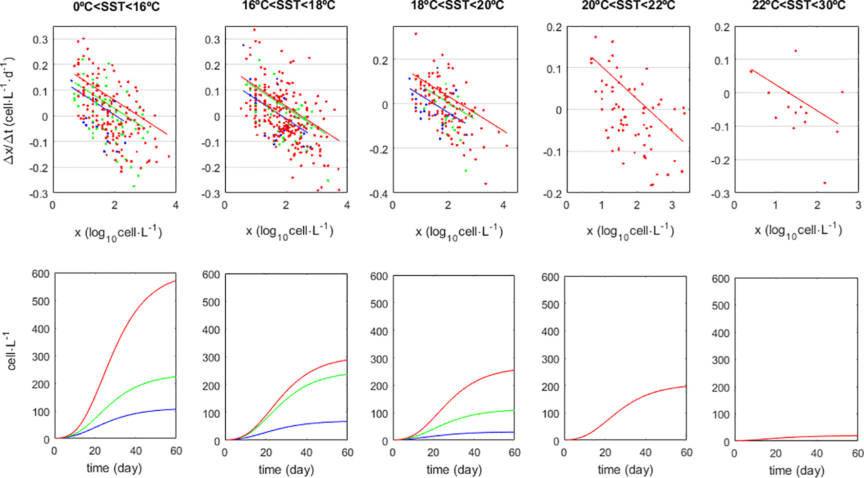
Figure 2 Sigmoid growth of Dyophysis acuminata populations and its dependency on Sea-Surface Temperature (SST) in °C, and Photosynthetic Active Radiation (PAR) corresponding to the flux of photons within the 400-700nm wavelengths observed at 12:00 (noon) and given in J·m^-2·h^-1. Colours correspond to PAR classes: (blue) PAR<6·10⁵, (green) 6·10⁶< PAR<9·10⁵, (red) 9·10⁵<PAR. Upper row panels: regression lines fit by Quantile Regression to the 75% percentile but using the pooled slope b=-0.078. Lower row panels: growth model simulations.

When modelling the D. acuminata population growth, the forecasted population size (n) at time t+Δt depended on its observed size at time t and on its growth rate (R). It was only the latter - the growth rate R - that depended on the environmental parameters averaged over the previous 5 days. Their effects can be visualized on the Δx/Δt-on-x plot (Figure 2; see Figures 2 and 3 in Vieira et al., 2021 for an example with macroalga). Any environmental factor significantly affecting the growth rate has a significant effect on the slope (b) and/or on the intercept (a) of the regression line.

The effects of environmental variables on D. acuminata growth were tested by ANCOVA. Each environmental variable was partitioned into classes (intervals). PAR (in J·m^-2·h^-1 as observed at 12:00 noon) was aggregated into Low (PAR<6·10⁶), Medium (6·10⁵< PAR<9·10⁵), and High (9·10⁵<PAR) classes that typically follow the seasonal cycle in higher latitudes as the North Atlantic. SST was aggregated into 2°C intervals between 16°C and 22°C, and open intervals beyond these bounds. This was considered the best solution to capture the signal in the data while not turning the amount of SST×PAR combinations overwhelming for the ANCOVA. A Δx/Δt-on-x regression was applied to the observations within each SST×PAR combination. These regressions were first compared for differences among estimated slopes (b). If slopes were significantly different, these and the respective intercepts (a) were preserved. If slopes were not significantly different, a pooled slope was estimated, applied to all classes, and then tested for differences among intercepts. The significances of the estimated slopes and intercepts where inferred by permutation tests using the Matlab software developed by Vieira and Creed (2013a), (2013b). The fundamental principle of permutation tests is that the null hypotheses are simulated by randomly redistributing the observations within each variable (thus breaking x-y correlations, to test for the significance of the slopes), and randomly redistributing the observations among classes (thus homogenizing classes, to test for the significance of the differences among slopes) (Manly, 1986). The permutation tests were performed with 10000 iterations i.e., the original plus 9999 simulations of the null hypothesis (randomizations). Estimation of coefficients (model calibration) by linear regression is highly sensitive to the regression methodology used (Pearson, 1901; Draper 1992; Smith, 2009; Vieira et al., 2016). We tested several regression methodologies: for model I regression were tested Ordinary Least Squares (OLS) and Quantile Regression (QR) (see Zhang et al., 2005; Creed et al., 2019, for QR and its application to ecological data). For model II regression were tested Principal Components Analysis (PCA) and Reduced Major Axis (RMA) (see Pearson, 1901; Draper 1992; Smith, 2009; Vieira et al., 2016, for types of model regression and their application to ecological data).

There are two ways to implement the model, diverging in the number of iterations performed to progress from the observed at time t to the forecasted for time t+Δt. One way is to do it in just one iteration. Considering the present case where Δt=7, the model implementation becomes n_t+7 = 10^{x+(a+b·x)·7}, with x=log₁₀n corresponding to the observed at time t. This implementation disregards that x evolves along the Δt=7 and with an impact on the final outcome (Figure 3). To account for this evolution, the x and Δx progression must be iterated along Δt. We did it in 7 iterations; one per day (Figure 3). The model implementation becomes n_t+1 = 10^x+(a+b·x) iterated 7 times, with the initial x₀=log₁₀n₀ corresponding the observation at time t=0 and the following x_i=log₁₀n_i corresponding to x forecasted by the previous iteration. This alternative, being more accurate, was preferred hereafter.

Figure 3

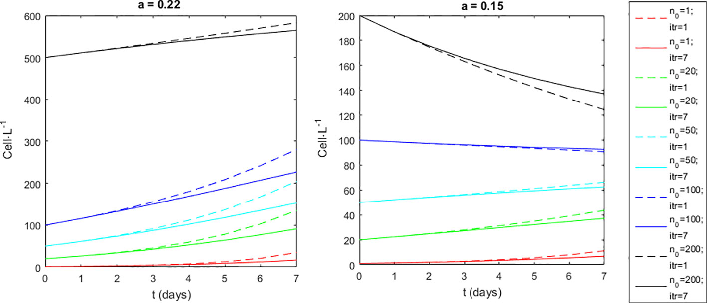
Figure 3 Alternative modes of model implementation. (Dashed lines) one iteration from t=0 to t=7 days. (Full lines) seven iterations (one per day) from t=0 to t=7 days. Initial conditions (n₀) tested were 1, 10, 50 100 and 500 cell·L^-1. Model implemented with a=0.15 or a=0.22, and b=-0.078.

3 Results

3.1 Environmental forcing of D. acuminata growth

The asymmetrical statistical distribution of some environmental variables together with the non-linear nature of their relations with D. acuminata growth (Figure 4) turned extremely difficult to access the strength and significance of these relations using standard statistical methods. An exploratory analysis showed that SST and PAR gave the best contributions to explain D. acuminata growth: population growth is favoured during lower temperatures and higher PAR periods, as shown by the colour scales on the respective panels (Figure 4) and the distribution of the Δx/Δt residuals (Figure 5). On the SST plot (Figure 4), warmer dominates towards the bottom of the data dispersion cloud whereas cooler dominates towards its top. On the PAR plot (Figure 4), observations taken under higher light intensity environments tend to place relatively higher along the data dispersion cloud relative to observations taken under lower light intensity environments. This was corroborated by the regression residuals of Δx/Δt (Figure 5), which tended to place upper under the combination of more intense PAR with cooler SST, and to place lower otherwise. Other variables were not relevant, as demonstrated by their even scatter along the data dispersion cloud (Figure 4). Following these results, the D. acuminata growth model was developed using SST and PAR as predictors. The higher growth rates obtained under high PAR and low SST should mainly occur during Spring-Summer upwelling conditions (Supplementary Figure S1). On the contrary, the lower growth rates obtained under low PAR and/or high SST report to distinct environmental scenarios. Considering the study area, low PAR and low SST correspond mainly to Winter conditions whereas medium/high PAR and high SST are associated with a variety of conditions from May to October without upwelling (Supplementary Figure S1).

Figure 4

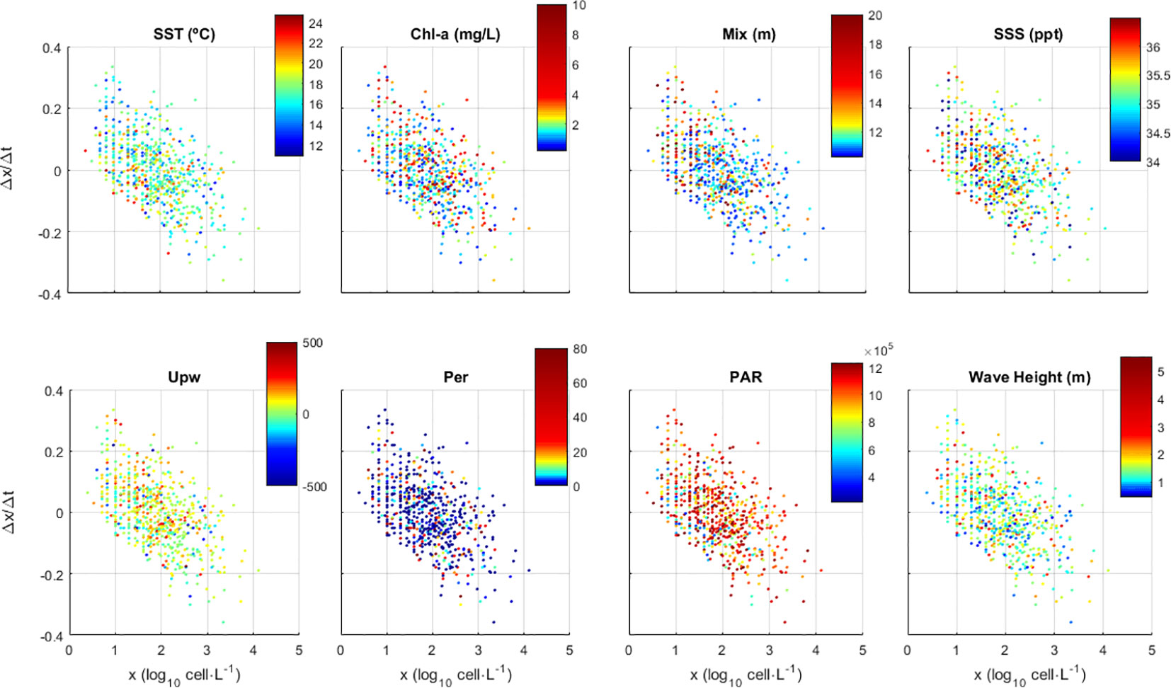
Figure 4 Effect of environmental variables on the population growth (Δx/Δt) of Dinophysis acuminata starting from an initial density x (x=log₁₀n, where n is cell·L^-1). Environmental variables where 5-day averaged, namely for Sea Surface Temperature (SST), Chlorophyl concentration (Chl), Mixed layer depth (Mix), Sea Surface Salinity (SSS), Bakun upwelling index (Upw), Precipitation (Per), Photosynthetic Active Radiation, (PAR) and Wave Height.

Figure 5

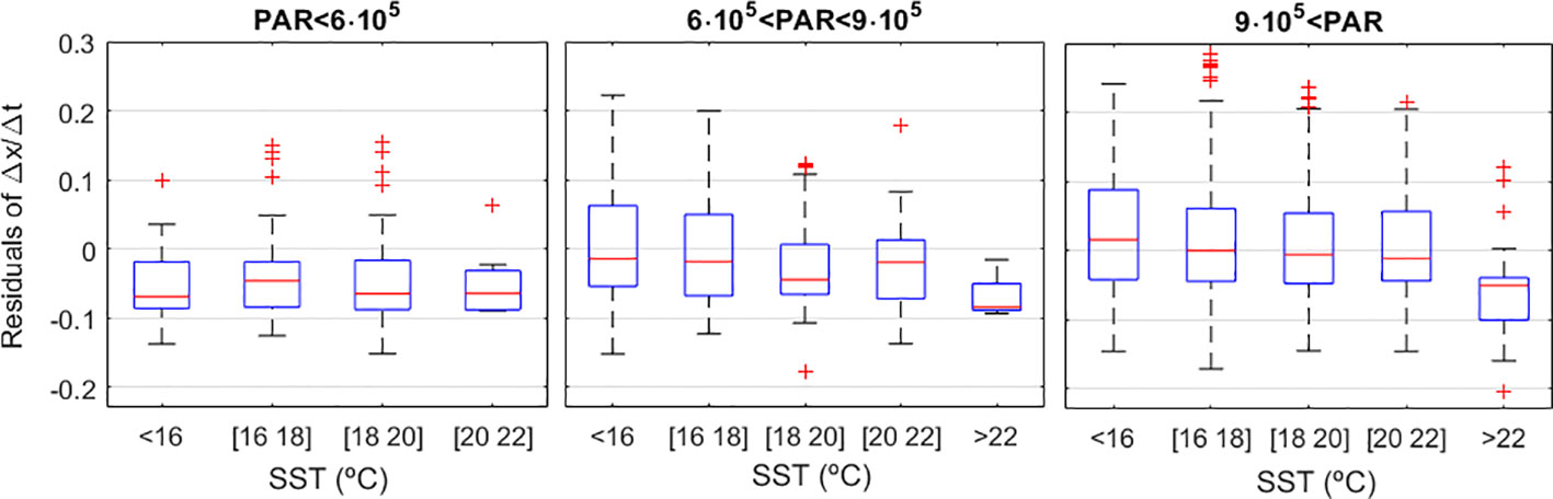
Figure 5 The Δx/Δt residuals and their dependency on PAR and SST. SST is Sea Surface Temperature in °C. PAR is Photosynthetic Active Radiation corresponding to the flux of photons within the 400-700nm wavelengths and given in mol·m^-2·s^-1. Red line (median), blue box (2^nd and 3^rd quartiles), whiskers (1^st and 4^th quartile), red crosses (outliers).

The ANCOVA compared among SST×PAR combinations. To each of these combinations was fit a regression line by Quantile regression using the 50% quantile. This ANCOVA showed that all slopes were significant (always p<0.0001, which is also much lower than the Bonferroni correction threshold). As for the differences between these slopes, the lowest p obtained was an isolated case of p=0.025, which is much higher than the Bonferroni correction for 55 pairwise comparisons (α=0.0009). Hence, it was considered that all slopes were statistically similar and decided to use the slope pooled among all slopes (b = -0.078). Inference about the differences between intercepts (a) revealed that many of them were largely different, both at the α=0.05 level or even at the Bonferroni correction level α=0.0009 (Figure 2; Table 1).

Table 1

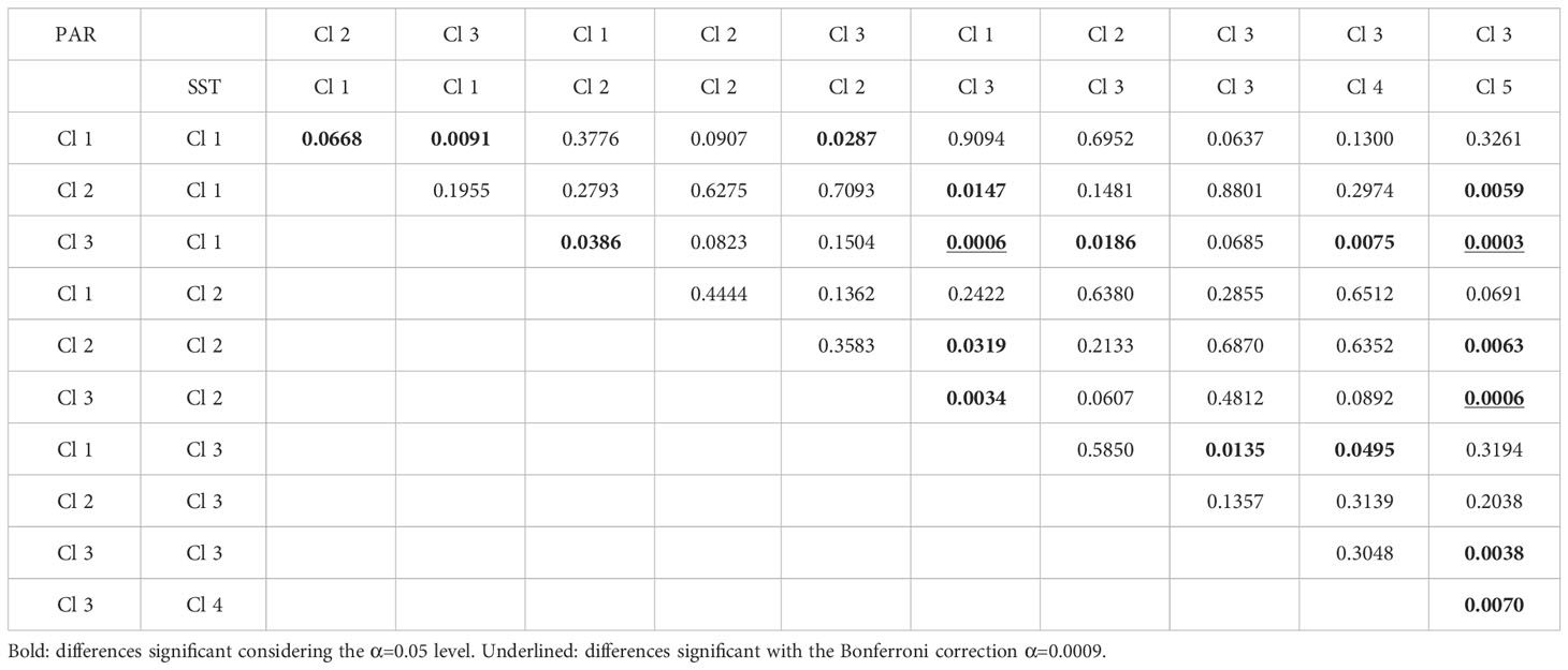
Table 1 Significance of differences between the intercepts estimated for the PAR×SST classes.

The results above suggest that the SST and PAR affected the maximum growth rate possible by D. acuminata (parameter a), whereas the decay of the maximum growth rate as the populations gets larger (parameter b) was unaffected.

3.2 Uncertainty analysis

Lateral advection and mixing - due to hydrodynamic processes such as eddies, fronts and turbulence - lead plankton to have patchy horizontal distributions at scales of 1-to-hundreds of meters (Martin, 2003; Pérez-Muñuzuri and Huhn, 2010). The importance of hydrodynamic transport processes in patch formation becomes more relevant as the time-scale of these processes becomes comparable (or shorter) to the time-scale of the phytoplankton reproduction (Okubo, 1978). Furthermore, species of the genus Dinophysis have been detected forming thin vertical layers in upwelling (Moita et al., 2006; Velo-Suarez et al., 2008) and fjord systems (Díaz et al., 2021). Because plankton distribution has high patchiness, its abundance data is commonly uncertain (e.g. Kiørboe, 1993). Therefore, we tested how this uncertainty affected the estimation of parameter a and its dependency on SST and PAR. For that, we estimated parameter a for all quantiles of the x-Δx/Δt bivariate distribution (Figure 6). The results confirmed that, despite all uncertainty in the data, D. acuminata grows better under the conjugation of higher PAR and cooler SST.

Figure 6

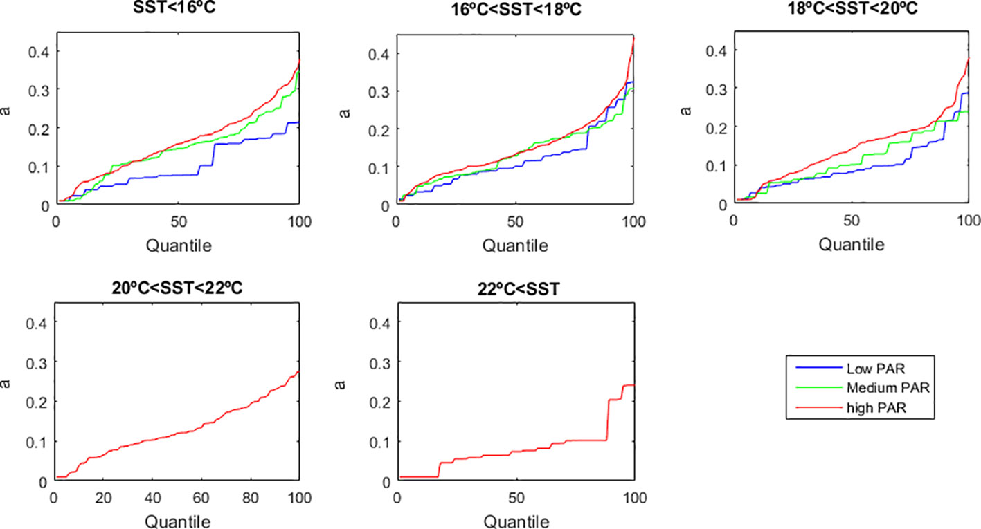
Figure 6 Uncertainty analysis upon the growth rate of D. acuminata. The quantile chosen for quantile regression affects the estimation of parameter a. SST is Sea Surface Temperature in °C. PAR is Photosynthetic Active Radiation.

Following the uncertainty analysis above, we tested running the D. acuminata growth model with the parameters a and b estimated from different quantiles. As an example, Figure 2 shows the growth function estimated from the quantile regression using the 75% quantile and Figure 7 shows the respective model run. Generally, forecasts fit well observations. Still, the uncertainty in the estimation of parameter a brought large uncertainty in the model performance (Figure 8).

Figure 7

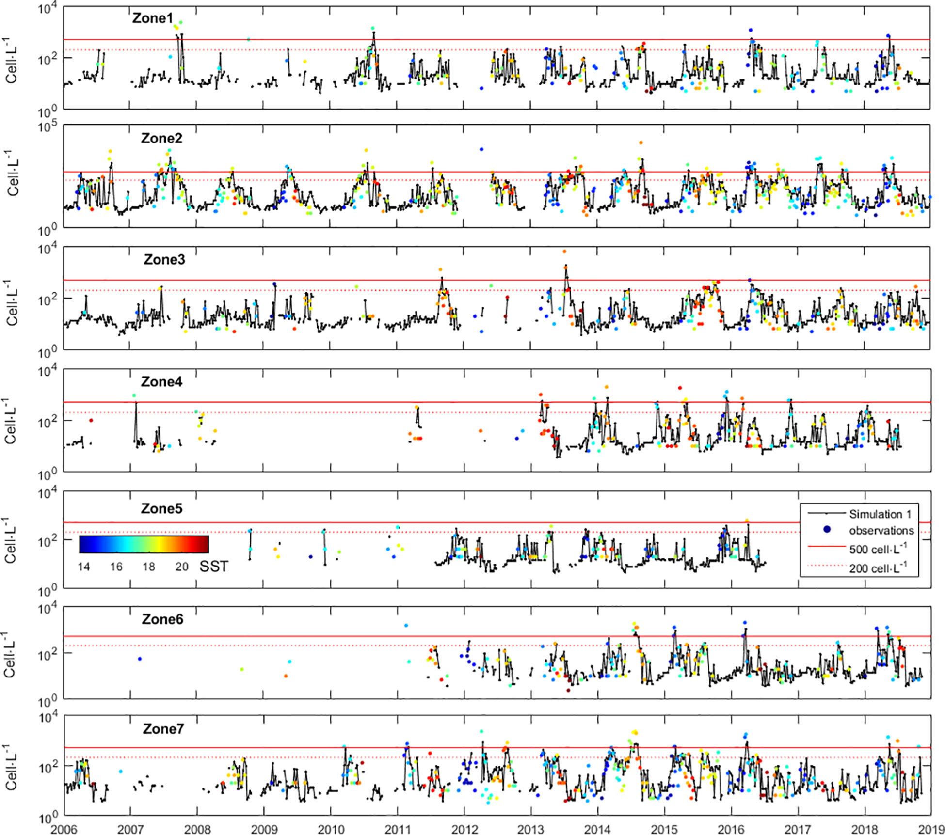
Figure 7 Timeseries of Dinophysis acuminata density in the 7 zones defined along the Portuguese coast, and model simulations with b=-0.078 and parameter a estimated from the 75% quantile.

Figure 8

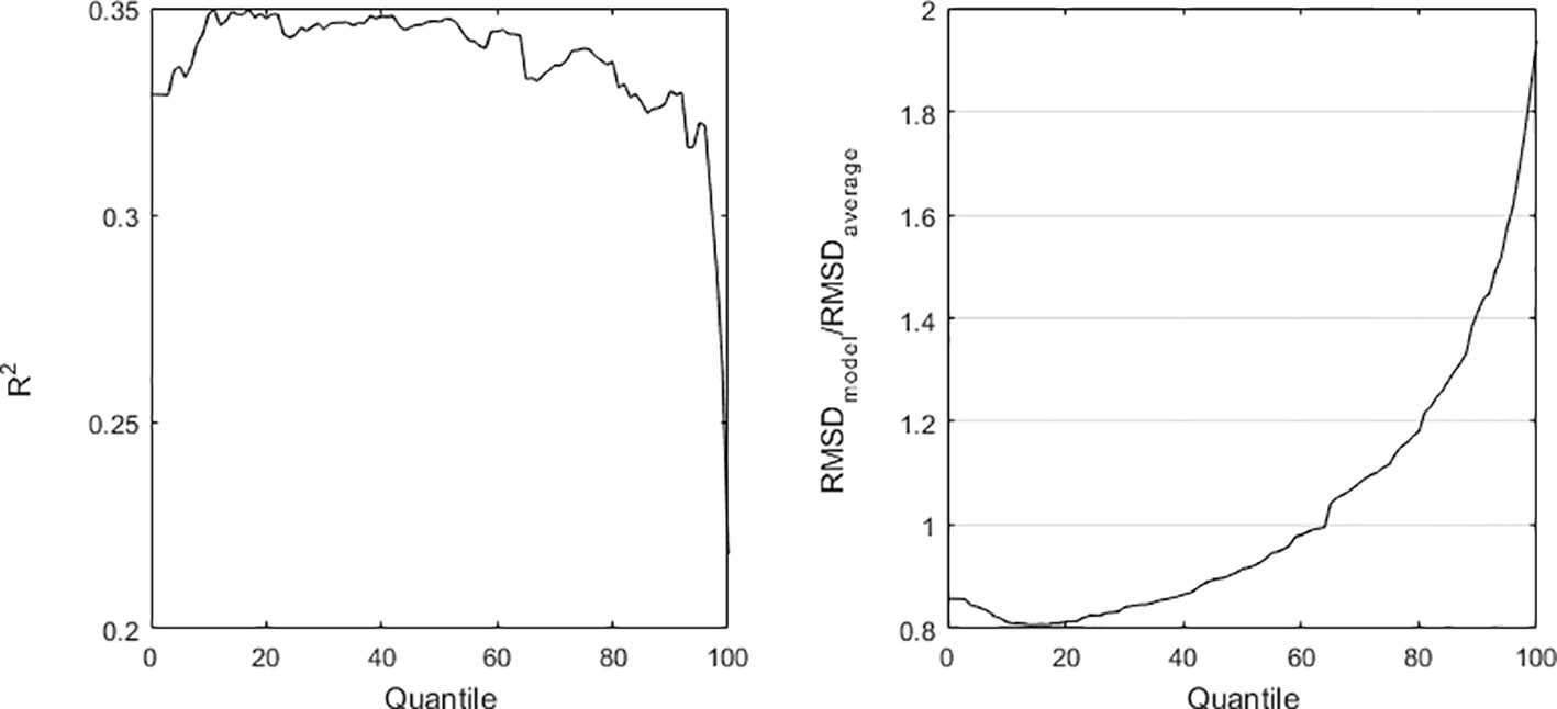
Figure 8 Uncertainty analysis regarding the D. acuminata growth model. The quantile chosen for quantile regression affects the estimation of the maximum growth rate (parameter a), which in its turn affects the model fit to observed data. Model fit to observed data is evaluated by R² and Root Mean Square Deviation (RMSD) applied to log cell·L^-1.

Minimizing the error in the estimates (in the numerical/statistical sense of ‘error’) does not necessarily provide the best decision on whether or not to emit a HAB warning given the 200 cell·L^-1 threshold, and whether or not to propose a precautionary closure of shellfish harvesting given the 500 cell·L^-1 threshold. In fact, the current model yield a correct warning decision probability p ≈ 0.89 and a correct precautionary closure probability p ≈ 0.94, depending on the monitoring zones. However, such apparently good results have problems. To illustrate these problems, we can conceptualize a given shellfish harvesting zone where 95% of the times the bivalve producers should not be closed. In such case, if the decision-taker adopts as effortless decision criterion to never close the harvesting under any circumstances, 95% of the times he shall be correct. Still, for the remaining 5% of the times, when closure is of utmost importance, he shall always fail. To improve the decision-making process, alternative criteria are required, namely, the probability of failing to emit a warning or failing to propose a precautionary closure (a false negative), and the probability of emitting a wrong warning or a wrong precautionary closure (a false positive). The model was re-evaluated according to these criteria. The uncertainty analysis showed that improving (i.e., minimizing) the probability of emitting a wrong warning or a wrong precautionary closure came at the cost of failing to emit a correct warning or a correct precautionary closure, and vice-versa (Figure 9).

Figure 9

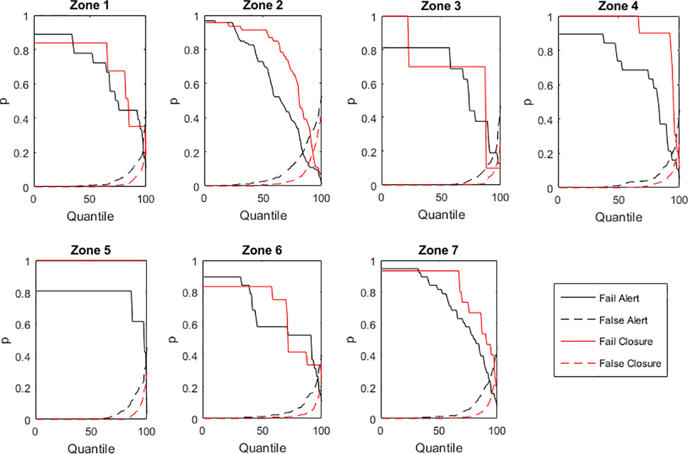
Figure 9 Uncertainty analysis upon the probabilities (p) of emitting HAB warnings or proposing harvesting closures.

3.3 Improving the forecasting ability

In this section it is shown that searching for the best model/numerical solution is secondary when facing the error introduced by the field and laboratorial methods, namely the too-wide time intervals between census and the detection limit of 20 cell·L^-1.

At the biological level, when conditions are favourable, D. acuminata grows at a pace that is too fast to be monitored (or modelled) at 7-day intervals. In fact, under favourable conditions, after 7 days the D. acuminata populations may grow to 5 times larger (Figures 2, 3). At the hydrodynamic level, when the sampler goes back to the same sampling station after 7 days, he can find a different water mass. The D. acuminata population previously sampled was subject to 7 days of advective transport, diffusion, and mixing. Consequently, even during D. acuminata blooms, consecutive samples taken from the same locations show high variability (Figure 7). The stated laboratory detection limit implies that any real cell density of microorganisms in the seawater below 20 cell·L^-1 was arbitrarily considered as 0 cell·L^-1 (actually, any value within 0 and 20 could be arbitrarily chosen). Arbitrarily setting these observations to zero disabled their use both for model estimation and model simulation because log₁₀0=-∞. From a modelling perspective, whatever the value arbitrarily chosen, these observations should not be used because they carry great uncertainty (or eventual bias). Besides being a problem for parameter estimation, this uncertainty was also a problem for model simulation. Any initial density (n_t) of 0 cell·L^-1 always remained 0 cell·L^-1 whatever the growth rate R. In order to run the model from those time instances, these observations needed to have arbitrarily attributed a value greater than zero and lower than 20 (i.e., 0<n_t<20). In theory, any value within these boundaries is equally acceptable. However, the consequences of choosing different values was significant. To understand the problem, consider the D. acuminata growth under the most favourable PAR and SST. If starting with 1 cell, after 7 days of growth, the result would be 17 cells, which was still under the detection limit. This may justify why, even under environmentally favourable conditions, observations of 0 cells·L^-1 were often followed by new observations of 0 cell·L^-1 at the next census. However, if starting with 19 cells, after 7 days of growth, the result would be 286 cells. This may justify why observations of 0 cell·L^-1 sometimes surprisingly burst to observations above the thresholds for warning at the next census. It was because all the conditions were met for that burst: the PAR, the SST and an initial population density that was big enough, although under a detection limit that is too high due to limited resources. To illustrate the broader effect of this bias (i.e., over all zones during the entire monitoring experiment), the model was first simulated with all original values of 0 cell·L^-1 being replaced by 1 cell·L^-1 (Figure 10 - Simulation 1). The simulation fit to observations, although failing in some situations. Then, all original values of 0 cell·L^-1 were instead replaced by 19 cell·L^-1, leading to a largely different model simulation (Figure 10 - Simulation 19).

Figure 10

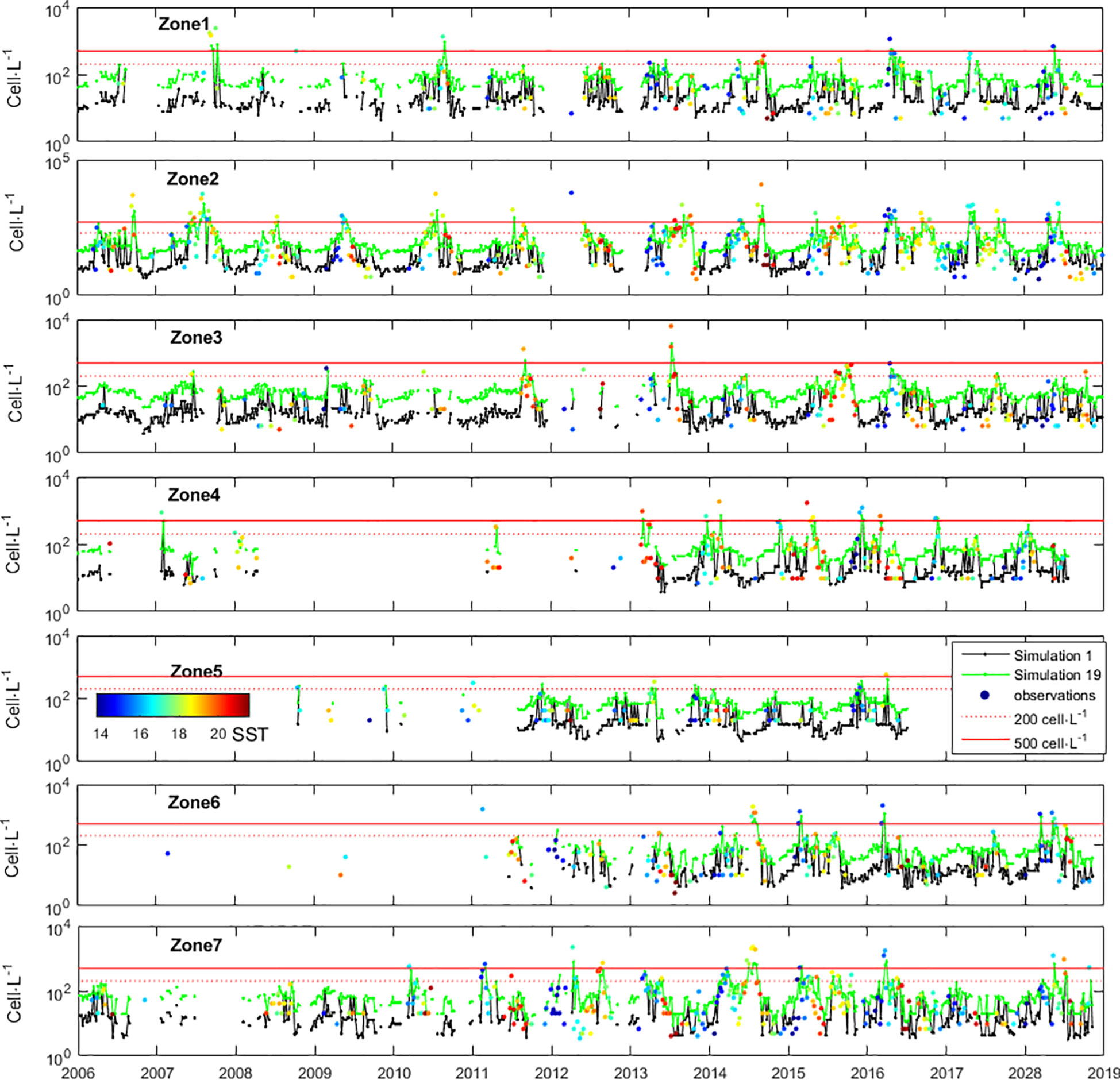
Figure 10 Timeseries of Dinophysis acuminata density in the 7 zones defined along the Portuguese coast, and model simulations. Simulation 1: initial observations of 0 cell·L^-1 arbitrarily replaced by 1 cell·L^-1. Simulation 19: initial observations of 0 cell·L^-1 arbitrarily replaced by 19 cell·L^-1.

4 Discussion

Our results suggest that D. acuminata thrives under the combination of high PAR and cool seawater. Given spring-summer light conditions, D. acuminata blooms with SST below 18°C. On the other hand, with SST above 20°C D. acuminata cannot bloom. These results fit the niche envelop previously reported for D. acuminata (e.g. Anschütz et al., 2022) as well as other Dinoflagellate species causing HABs in the North Atlantic (Gianella et al., 2021; Lima et al., 2022). These favourable conditions correspond to the spring-summer upwelling regime characterized by bright sunny days and nutrient-rich cold waters, typical to the Iberian and Morocco coastal ocean (Ambar and Dias, 2008; Alvarez et al., 2010; Díaz et al., 2013, 2016; Moita et al., 2016; Leitão et al., 2019; Danchenko et al., 2022). In other locations on the North Atlantic, namely along the Bay of Biscay, British Isles and British Channel, the water is cold enough due to its higher latitude. Consequently, the summer is the typical season for HAB of D. acuminata as well as other Dinoflagellate species in the North Atlantic (Smayda and Trainer, 2010; Díaz et al., 2013, 2016; Moita et al., 2016; Swan et al., 2018; Fernández et al., 2019; Gianella et al., 2021; Danchenko et al., 2022; Lima et al., 2022).

Despite the environmental conditions favouring HABs being already reasonably understood, attempts to systematically forecast them have underachieve. Often, these attempts considered the modelling of HABs as a strictly statistical problem requiring a strictly statistical solution. Consequently, statistical tools were applied to produce empirical models forecasting the population size from environmental predictors. By doing so, these attempts incurred in two flaws: first, to choose population size as response variable when the correct choice should be the population growth rate; second, neglecting the fundamental factor in demographic forecasting that is “how much was there to start with?” i.e., the initial population size. It is known that numerous phytoplankton species can double their population in 12h under good environmental conditions (e.g. Smayda, 1997); if there is 1 cell to start with, the day after we have 4 cells. But if there are 1000 cells to start with, the day after we have 4000 cells. Our simulations with D. acuminata illustrated well these aspects and the results are evidence that forecasting HABs is a problem of population dynamics/demography. Hence, the solution must come from population dynamics/demography theory and respective mechanistic models. These say that environmental factors set the population growth rate and the maximum sustainable population size, also known as “carrying capacity”. Hence, in the simplest approach possible, the correct choice for response variable is the population growth rate. In a more elaborate approach, as we did in this work, the environmental predictors affect the population growth rate dependency from current population size i.e., how the initially exponential growth dampens as the population approaches its carrying capacity. It is only at this stage (i.e., once the core model has been established from population dynamics/demography theory) that statistics steps in to fit the dependency of demographic parameters from environmental predictors; and for that fit there are many viable statistical alternatives.

Like many dinoflagellates (see Smayda, 1997), D. acuminata is a mixotrophic species (Anschütz et al., 2022): a phagotroph acquiring phototrophy from the Mesodinium it preys upon, in its turn acquiring phototrophy from the Teleaulax it preys upon. This sequence is known as the Teleaulax-Mesodinium-Dinophysis-Complex. Given the D. acuminata sensibility to the light environment and its phototrophy being acquired from its prey, demographic models shall predict better D. acuminata growth if they also take into consideration the availability of Mesodinium. The fact that the niche envelops of both predator and prey are similar (see Anschütz et al., 2022) facilitates this task. Nevertheless, the onset of the right environmental conditions should not immediately trigger a D. acuminata bloom as a prior bloom of Mesodinium is likely required (see Moita et al., 2016). Unfortunately, weekly data on Teleaulax and Mesodinium are not available in the study area. Hence, we could not include them in our modelling. Still, we recognize that these predator-prey dynamics and the time-lag between prey bloom and the following predator bloom may justify why the D. acuminata growth was better forecasted from the environmental data relative to the previous 5 days, rather than from the simultaneous data. Once the monitoring constrains by us identified are solved, modelling the Teleaulax-Mesodinium-Dinophysis-Complex will become the fundamental development for accurate forecasting of D. acuminata blooms.

This work identified the necessary knowledge about D. acuminata ecology and population dynamics so that this is no longer a limitation to forecasting its blooms. The results also indicate that for this knowledge to be effective it must be applied to input data with better resolution. While this is not improved, forecasts will continue limited and attempts to develop better models are probably futile. The first key issues lessening the adequacy of the input data was the census intervals of 7 days that proved to be too wide to monitor D. acuminata populations when environmental conditions were favourable for their growth (Figures 2, 3, 7). Even starting from low numbers, after 7 days of favourable growth their populations can overshoot the 500 cell·L^-1 threshold representing a harmful abundances for shellfish toxification. Knowing D. acuminata has relatively low inherent growth rates compared to many other HAB species, our results quantitatively confirm the severe insufficiency of 7-day census for most microbiological processes. When modelling population growth, the simulations may overshoot reality, and even became unstable or chaotic, because a continuous process was modelled as being discrete and with too large time intervals (Akçakaya et al., 1999; Caswell, 2001). The importance of monitoring and modelling HABs with time resolutions shorter than 7 days was actually demonstrated by the significant improvements in south Florida’s operational monitoring program when the monitoring was performed twice-daily and in the operational forecast system when the model was run twice-weekly (Stumpf et al., 2009). The second key issue lessening the adequacy of the input data was the laboratory detection limit of 20 cells·L^-1. Our work proved this limit to be too coarse to monitor D. acuminata populations when environmental conditions were favourable for their growth. Below the detection limit, the actual in situ population numbers were unknown, with 0 or 19 cell·L^-1 being equally likely yet producing opposing results (Figure 10). Starting the model with 1 or 19 cells can result after 7 days in an incipient population or an overshoot of the HAB alarm threshold (200 cell·L^-1), which is problematic for an operational shellfish toxicity monitoring program that needs to communicate accurate information.

Even good demographic models applied to high resolution data underachieve forecasting HABs if they do not take into account the motion of the ocean water with the consequent advection and diffusion of the phytoplankton cells. For this reason, the state-of-the-art in forecasting HABs use hydrodynamic simulations to force Lagrangian simulations of phytoplankton dispersion. Such are the cases of HABs forecasting in the North Atlantic, namely along the Iberian shelf, Bay of Biscay, British Isles and British Channel (Bedington et al., 2022; Hariri et al., 2022). Cell multiplication is the fundamental determinant of HABs during their earlier stages. However, when populations have already achieved densities that are high and/or harmful, their transport and dispersion gain importance for the accuracy of the forecasts (Bedington et al., 2022). A significant portion of the lack of accuracy in our modelling efforts resulted from the lack of hydrodynamics in our model and this was exacerbated by a too wide census/projection interval. Over the course of 7 days, advective transportation could carry D. acuminata cells towards or away from each of census location whereas diffusion processes and/or sinking losses could locally alter its cell density in a specific volume of water. This was challenging both for monitoring and for forecasting. In the case of monitoring, it brought great uncertainty about how much of the change in the observed population numbers resulted from its “local” biology and how much resulted from larger scale hydrodynamics. Given this uncertainty, it was very hard to estimate model coefficients with confidence. In the case of forecasting, even if we had a perfect demographic model to forecast cell multiplication, not knowing where those cells headed turned very difficult to produce accurate forecasts.

The too wide census/projection intervals, the coarse detection limit and the neglection of hydrodynamics are probably behind the unexpected surge in D. acuminata numbers following situations of perceived absence. Improving these aspects demands substantial increase in the sampling logistics, laboratory methods and modelling efforts, which is difficult if the resources of any given HAB monitoring program are not increased. For future work in this field, we suggest two solutions. One, is to use image acquisition systems (both in situ and laboratory hardware units) with machine learning software to automate the counting of phytoplankton cells and therefore increase sample processing and lower the detection limit. The other is to intensify the seawater collection effort only when conditions are favourable for any given HAB species. Considering D. acuminata, this sampling intensification should take place during the upwelling regime that takes place along the western Iberian shelf mainly during the summer season (Ambar and Dias, 2008; Alvarez et al., 2010; Leitão et al., 2019; Danchenko et al., 2022). Hence, weather forecasts of incoming north winds leading to upwelling, and the subsequent cooling of SST, may be used as triggers (in some semi-automatic way) to intensify the sampling effort, as well as to relax the remaining time. A time-variable monitoring programme maybe the key to optimize the prediction of D. acuminata blooms, as well as other HAB species, and obtain forecasts of the highest quality, helping effective management measures for the shellfish industry.

Data availability statement

The raw data supporting the conclusions of this article will be made available by the authors, without undue reservation.

Author contributions

VV: Software, Methodology, Investigation, Formal analysis, Writing – original draft, Visualization, Validation. TLR: Writing – review & editing, Resources, Methodology, Investigation, Data curation, Conceptualization. LS-G: Writing – review & editing, Supervision, Resources, Project administration, Methodology, Investigation, Funding acquisition, Data curation, Conceptualization. MM: Writing – review & editing, Resources, Project administration, Funding acquisition. BM: Writing – review & editing, Resources, Methodology, Formal analysis, Data curation, Conceptualization.

Funding

The author(s) declare financial support was received for the research, authorship, and/or publication of this article. This research was funded by the European Maritime, Fisheries Fund, under the MAR2020 program, through project SNMB-MONITOR National Monitoring Program for Marine Toxins in Bivalves Molluscs (MAR2020-02-01-02-FEAMP-0043), by Interreg Atlantic Area Programme Project PRIMROSE (Grant No. EAPA_182/2016, https://www.shellfish-safety.eu/) and by FCT - Foundation for Science and Technology through projects UIDB/04326/2020 (DOI:10.54499/UIDB/04326/2020), UIDP/04326/2020 (DOI:10.54499/UIDP/04326/2020) and LA/P/0101/2020 (DOI:10.54499/LA/P/0101/2020). TLR was supported by the research grant IPMA-2018-04-BI.

Conflict of interest

The authors declare that the research was conducted in the absence of any commercial or financial relationships that could be construed as a potential conflict of interest.

Publisher’s note

All claims expressed in this article are solely those of the authors and do not necessarily represent those of their affiliated organizations, or those of the publisher, the editors and the reviewers. Any product that may be evaluated in this article, or claim that may be made by its manufacturer, is not guaranteed or endorsed by the publisher.

Supplementary material

The Supplementary Material for this article can be found online at: https://www.frontiersin.org/articles/10.3389/fmars.2024.1355706/full#supplementary-material

References

Akçakaya H. R., Burgman M. A., Ginzburg L. R. (1999). Applied population ecology. 2nd Edition (Sunderland, Massachusetts: Sinauer Associates).

Google Scholar

Alvarez I., Gomes-Gesteira M., de Castro M., Lorenzo M. N., Crespo A. J. C., Dias J. M. (2010). Comparative analysis of upwelling influence between the western and northern coast of the Iberian Peninsula. Continental Shelf Res. 31, 388–399. doi: 10.1016/j.csr.2010.07.009

CrossRef Full Text | Google Scholar

Ambar I., Dias J. (2008). “Remote sensing of coastal upwelling in the North-Eastern Atlantic Ocean,” in Remote Sensing of the European Seas. Eds. Barale V., Gade M. (Springer, Dordrecht). doi: 10.1007/978-1-4020-6772-3_11

CrossRef Full Text | Google Scholar

Anderson D. M. (2009). Approaches to monitoring, control and management of harmful algal blooms (HABs). Ocean Coast. Manage. 52, 342. doi: 10.1016/j.ocecoaman.2009.04.006

CrossRef Full Text | Google Scholar

Anderson C. R., Moore S. K., Tomlinson M. C., Silke J., Cusack C. K. (2015). “Chapter 17 - living with harmful algal blooms in a changing world: strategies for modeling and mitigating their effects in coastal marine ecosystems,” in Hazards and Disasters Series, Coastal and Marine Hazards, Risks, and Disasters. Eds. Shroder J. F., Ellis J. T., Sherman D. J. (Elsevier), 2015, 495–561. doi: 10.1016/B978-0-12-396483-0.00017-0

CrossRef Full Text | Google Scholar

Anschütz A.-A., Flynn K. J., Mitra A. (2022). Acquired phototrophy and its implications for bloom dynamics of the teleaulax-mesodinium-dinophysis-complex. Front. Mar. Sci. 8. doi: 10.3389/fmars.2021.799358

CrossRef Full Text | Google Scholar

Bedington M., García-García L. M., Sourisseau M., Ruiz-Villarreal M. (2022). Assessing the performance and application of operational lagrangian transport HAB forecasting systems. Front. Mar. Sci. 9. doi: 10.3389/fmars.2022.749071

PubMed Abstract | CrossRef Full Text | Google Scholar

Caswell H. (2001). Matrix Population Models: Construction, Analysis and Interpretation (Sunderland, Massachusetts: Sinauer Associates), 722 pp.

Google Scholar

Creed J., Vieira V. M. N. C. S., Norton T. A., Caetano D. (2019). A meta-analysis shows that seaweeds surpass plants, setting life-on-Earth’s limit for biomass packing. BMC Ecol. 19 (6), 1–11. doi: 10.1186/s12898-019-0218-z

CrossRef Full Text | Google Scholar

Cunha M. E. (2001). Physical control of biological processes in a coastal upwelling system: comparison of the effects of coastal topography, river run-off and physical oceanography in the northern and southern parts of Western Portuguese Coastal Waters. Faculdade de Ciências da Universidade de Lisboa, Lisbon, Portugal. Ph.D. Thesis.

Google Scholar

Danchenko S., Dodge J., Icely J., Newton A. (2022). Dinoflagellate assemblages in the West Iberian upwelling region (Sagres, Portugal) during 1994–2001. Front. Mar. Sci. 9. doi: 10.3389/fmars.2022.591759

PubMed Abstract | CrossRef Full Text | Google Scholar

Díaz P. A., Pérez-Santos I., Álvarez G., Garreaud R., Pinilla E., Díaz M., et al. (2021). Multiscale physical background to an exceptional harmful algal bloom of Dinophysis acuta in a fjord system. Sci. Total Environ. 773, 145621. doi: 10.1016/j.scitotenv.2021.145621

PubMed Abstract | CrossRef Full Text | Google Scholar

Díaz P. A., Reguera B., Ruiz-Villarreal M., Pazos Y., Velo-Suárez L., Berger H., et al. (2013). Climate variability and oceanographic settings associated with interannual variability in the initiation of Dinophysis acuminata blooms. Mar. Drugs 11, 2964–2981. doi: 10.3390/md11082964

PubMed Abstract | CrossRef Full Text | Google Scholar

Díaz P. A., Ruiz-Villarreal M., Pazos Y., Moita T., Reguera B. (2016). Climate variability and Dinophysis acuta blooms in an upwelling system. Harmful Algae 53, 145–159. doi: 10.1016/j.hal.2015.11.007

PubMed Abstract | CrossRef Full Text | Google Scholar

Draper N. R. (1992). Straight line regression when both variables are subject to error. In: Milliken GH., Schwenke JR. (eds). Proceedings of the Conference on Applied Statistics in Agriculture, 28–30 April 1991, Kansas State University. Manhattan, KS: Kansas StateUniversity. 1–18.

Google Scholar

Fan Y., Li W., Gatebe C. K., Jamet C., Zibordi G., Schroeder T., et al. (2017). Atmospheric correction over coastal waters using multilayer neural networks. Remote Sens. Environ. 199, 218–240. doi: 10.1016/j.rse.2017.07.016

CrossRef Full Text | Google Scholar

FAO, IOC, IAEA. (2023). “Joint technical guidance for the implementation of early warning systems for harmful algal blooms,” in Fisheries and Aquaculture Technical Paper No. 690 (FAO, Rome). doi: 10.4060/cc4794en

CrossRef Full Text | Google Scholar

Fernández R., Mamán L., Jaén D., Fuentes L. F., Ocaña M. A., Gordillo M. M. (2019). Dinophysis species and diarrhetic shellfish toxins: 20 years of monitoring program in Andalusia, South of Spain. Toxins (Basel). 11, 189. doi: 10.3390/toxins11040189

PubMed Abstract | CrossRef Full Text | Google Scholar

Gianella F., Burrows M. T., Swan S. C., Turner A. D., Davidson K. (2021). Temporal and spatial patterns of harmful algae affecting Scottish shellfish aquaculture. Front. Mar. Sci. 8. doi: 10.3389/fmars.2021.785174

CrossRef Full Text | Google Scholar

Gompertz B. (1825). On the nature of the function expressive of the law of human mortality, and on a new mode of determining the value of life contingencies. Philos. Trans. R. Soc. London 115, 513–585. doi: 10.1098/rstl.1825.0026

CrossRef Full Text | Google Scholar

Hariri S., Plus M., Le Gac M., Séchet V., Revilla M., Sourisseau M. (2022). Advection and composition of dinophysis spp. Populations along the European Atlantic shelf. Front. Mar. Sci. 9. doi: 10.3389/fmars.2022.914909

PubMed Abstract | CrossRef Full Text | Google Scholar

Ilori C., Pahlevan N., Knudby A. (2019). Analyzing performances of different atmospheric correction techniques for landsat 8: application for coastal remote sensing. Remote Sens. 11, 469. doi: 10.3390/rs11040469

CrossRef Full Text | Google Scholar

Kiørboe T. (1993). Turbulence, phytoplankton cell size, and the structure of pelagic food webs. Adv. Mar. Biol. 29, 1–72. doi: 10.1016/S0065-2881(08)60129-7

CrossRef Full Text | Google Scholar

Kudela R., Berdalet E., Bernard S., Burford M., Fernand L., Lu S., et al. (2015). Harmful Algal Blooms. A scientific summary for policy makers (Paris (IOC/INF-1320: IOC/UNESCO).

Google Scholar

Leitão F., Baptista V., Vieira V., Laginha Silva P., Relvas P., Teodósio M. A. (2019). A 60-year time series analyses of the upwelling along the portuguese coast. Water 11, 1285. doi: 10.3390/w11061285

CrossRef Full Text | Google Scholar

Lima M. J., Relvas P., Barbosa A. B. (2022). Variability patterns and phenology of harmful phytoplankton blooms off southern Portugal: Looking for region-specific environmental drivers and predictors. Harmful Algae 116, 102254. doi: 10.1016/j.hal.2022.102254

PubMed Abstract | CrossRef Full Text | Google Scholar

Lundholm N., Churro C., Escalera L., Fraga S., Hoppenrath M., Iwataki M., et al. (2009). IOC-UNESCO Taxonomic Reference List of Harmful Micro Algae. Available at: https://www.marinespecies.org/hab (Accessed 2023-03-30).

Google Scholar

Lu Z., Li J., Shen Q., Zhang B., Zhang H., Zhang F., et al. (2018). Modification of 6SV to remove skylight reflected at the air-water interface: Application to atmospheric correction of Landsat 8 OLI imagery in inland waters. PLoS One. 24;13 (8), e0202883. doi: 10.1371/journal.pone.0202883

CrossRef Full Text | Google Scholar

Manly B. J. F. (1986). Multivariate methods. Chapman & Hall, London, United Kingdom.

Google Scholar

Martin A. P. (2003). Phytoplankton patchiness: the role of lateral stirring and mixing. Prog. Oceanogr. 57, 125–174. doi: 10.1016/S0079-6611(03)00085-5

CrossRef Full Text | Google Scholar

Moita M. T., Pazos Y., Rocha C., Nolasco R., Oliveira P. B. (2016). Toward predicting Dinophysis blooms off NW Iberia: A decade of events. Harmful Algae. 53, 17–32. doi: 10.1016/j.hal.2015.12.002

PubMed Abstract | CrossRef Full Text | Google Scholar

Moita M. T., Sobrinho-Gonçalves L., Oliveira P. B., Palma S., Falcão M. (2006). A bloom of Dinophysis acuta in a thin layer off NW Portugal. Afr. J. Mar. Sci. 28, 265–269. doi: 10.2989/18142320609504160

CrossRef Full Text | Google Scholar

Okubo A. (1978). “Horizontal dispersion and critical scales for phytoplankton patches,” in Spatial Pattern in Plankton Communities, vol. 3 . Ed. Steele J. H. (Springer, Boston, MA). doi: 10.1007/978-1-4899-2195-6_2

CrossRef Full Text | Google Scholar

Otero P., Ruiz-Villarreal M., And Peliz A. (2008). Variability of river plumes off Northwest Iberia in response to wind events. J. Mar. Syst. 72, 238–255. doi: 10.1016/j.jmarsys.2007.05.016

CrossRef Full Text | Google Scholar

Paine C. E. T., Marthews T. R., Vogt D. R., Purves D., Rees M., Hector A., et al. (2012). How to fit nonlinear plant growth models and calculate growth rates: an update for ecologists. Methods Ecol. Evolution. 3, 245–256. doi: 10.1111/j.2041-210X.2011.00155.x

CrossRef Full Text | Google Scholar

Pearson K. (1901). On lines and planes of closest fit to systems of points in space. Philos. Mag. 2, 559–572. doi: 10.1080/14786440109462720

CrossRef Full Text | Google Scholar

Peliz A., Rosa T. L., Santos A. M., Pissarra J. L. (2002). Fronts, jets, and counter-f lows in the Western Iberian upwelling system. J. Mar. Syst. 35, 61–77. doi: 10.1016/S0924-7963(02)00076-3

CrossRef Full Text | Google Scholar

Pérez-Muñuzuri V., Huhn F. (2010). The role of mesoscale eddies time and length scales on phytoplankton production. Nonlinear Process. Geophys. 17, 177–186. doi: 10.5194/npg-17-177-2010

CrossRef Full Text | Google Scholar

Reguera B., Alonso R., Moreira A., Méndez S., Dechraoui-Bottein M.-Y. (2016). Guide for Designing and Implementing a Plan to Monitor Toxin-Producing Microalgae. 2nd ed Vol. 2 (Paris, France: IOC), 66.

Google Scholar

Reguera B., Riobó P., Rodríguez F., Díaz P. A., Pizarro G., Paz B., et al. (2014). Dinophysis toxins: causative organisms, distribution and fate in shellfish. Mar. Drugs 12, 394–461. doi: 10.3390/md12010394

PubMed Abstract | CrossRef Full Text | Google Scholar

Shen L., Xu H., Guo X. (2012). Satellite remote sensing of harmful algal blooms (HABs) and a potential synthesized framework. Sens. (Basel). 12, 7778–7803. doi: 10.3390/s120607778

CrossRef Full Text | Google Scholar

Smayda T. J. (1997). Harmful algal blooms: Their ecophysiology and general relevance to phytoplankton blooms in the sea. Limnol. Oceanogr. 42, 1137–1153. doi: 10.4319/lo.1997.42.5_part_2.1137

CrossRef Full Text | Google Scholar

Smayda T. J., Trainer V. L. (2010). Dinoflagellate blooms in upwelling systems: Seeding, variability, and contrasts with diatom bloom behaviour. Prog. Oceanogr. 85, 92–107. doi: 10.1016/j.pocean.2010.02.006

CrossRef Full Text | Google Scholar

Smith R. J. (2009). Use and misuse of Reduced Major Axis for line-fitting. Am. J. Phys. Anthropol. 140, 476–486. doi: 10.1002/ajpa.21090

PubMed Abstract | CrossRef Full Text | Google Scholar

Smith M. E., Bernard S. (2020). Satellite ocean color based harmful algal bloom indicators for aquaculture decision support in the Southern Benguela. Front. Mar. Sci. 7. doi: 10.3389/fmars.2020.00061

CrossRef Full Text | Google Scholar

Stumpf R., Fleming V., Granéli E. (2010). Integration of data for nowcasting of harmful algal blooms. In OceanObs’09 Conference Proceedings. 21–25 September 2009. Venice, Italy. doi: 10.5270/OceanObs09.pp.36

CrossRef Full Text | Google Scholar

Stumpf R. P., Tomlinson M. C., Calkins J. A., Kirkpatrick B., Fisher K., Nierenberg K., et al. (2009). Skill assessment for an operational algal bloom forecast system. J. Mar. Syst. 76, 151–161. doi: 10.1016/j.jmarsys.2008.05.016

PubMed Abstract | CrossRef Full Text | Google Scholar

Swan S. C., Turner A. D., Bresnan E., Whyte C., Paterson R. F., McNeill S., et al. (2018). Dinophysis acuta in Scottish coastal waters and its influence on diarrhetic shellfish toxin profiles. Toxins (Basel) 10, 399. doi: 10.3390/toxins10100399

PubMed Abstract | CrossRef Full Text | Google Scholar

Trainer V. L., Pitcher G. C., Reguera B., Smayda T. J. (2010). The distribution and impacts of harmful algal bloom species in eastern boundary upwelling systems. Prog. Oceanogr. 85, 33–52. doi: 10.1016/j.pocean.2010.02.003

CrossRef Full Text | Google Scholar

Utermohl H. (1958). Zur Ver vollkommung der quantitativen phytoplankton-methodik. Mitteilung Internationale Vereinigung Fuer Theoretische unde Amgewandte. Limnol. 9, 1–38. doi: 10.1080/05384680.1958.11904091

CrossRef Full Text | Google Scholar

Vale P., Botelho M. J., Rodrigues S. M., Gomes S. S., Sampayo M. A. M. (2008). Two decades of marine biotoxin monitoring in bivalves from Portugal, (1986-2006): a review of exposure assessment. Harmful Algae 7, 11–25. doi: 10.1016/j.hal.2007.05.002

CrossRef Full Text | Google Scholar

Velo-Suárez L., González-Gil S., Gentien P., Lunven M., Bechemin B., Fernand L., et al. (2008). Thin layers of Pseudo-nitzschia spp. and the fate of Dinophysis acuminata during an upwelling-downwelling cycle in a Galician Ría. Limnol. Oceanogr. 53, 1816–1834. doi: 10.4319/lo.2008.53.5.1816

CrossRef Full Text | Google Scholar

Vieira V. M. N. C. S., Creed J. (2013a). Estimating signifcances of diferences between slopes: A new methodology and software. Comput. Ecol. Softw. 3, 44–52.

Google Scholar

Vieira V. M. N. C. S., Creed J. (2013b). Signifcances of diferences between slopes: An upgrade for replicated time series. Comput. Ecol. Softw. 3, 102–109.

Google Scholar

Vieira V. M. N. C. S., Creed J., Scrosati R. A., Santos A., Dutschke G., Leitão F., et al. (2016). On the choice of linear regression algorithms. Annu. Res. Rev. Biol. 10, 1–9. doi: 10.9734/arrb/2016/25219

CrossRef Full Text | Google Scholar

Vieira V. M. N. C. S., Engelen A. H., Huanel O. R., Guillemin M.-L. (2018). Haploid females in the isomorphic biphasic life-cycle of Gracilaria Chilensis excel in survival. BMC Evol. Biol. 18, 174. doi: 10.1186/s12862-018-1285-z

PubMed Abstract | CrossRef Full Text | Google Scholar

Vieira V. M. N. C. S., Engelen A. H., Huanel O., Guillemin M.-L. (2021). Differential frond growth in the isomorphic haploid-diploid red seaweed Agarophyton Chilense by long-term in situ monitoring. J. Phycol. 57, 592–605. doi: 10.1111/jpy.13110

PubMed Abstract | CrossRef Full Text | Google Scholar

Vieira V. M. N. C. S., Engelen A. H., Huanel O. R., Guillemin M.-L. (2022). An individual-based model of the red alga agarophyton Chilense unravels the complex demography of its intertidal stands. Front. Ecol. Evol. 10. doi: 10.3389/fevo.2022.797350

CrossRef Full Text | Google Scholar

Wang X., Bouzembrak Y., Marvin H. J. P., Clarke D., Butler F. (2022). Bayesian Networks modeling of diarrhetic shellfish poisoning in Mytilus edulis harvested in Bantry Bay, Ireland. Harmful Algae 12, 102171. doi: 10.1016/j.hal.2021.102171

CrossRef Full Text | Google Scholar

Weibull W. (1951). A statistical distribution function of wide applicability. J. Appl. Mechanics 18, 293–297. doi: 10.1115/1.4010337

CrossRef Full Text | Google Scholar

Winsor C. P. (1932). The Gompertz curve as a growth curve. Proc. Natl. Acad. Sci. U.S.A. 18, 1–8. doi: 10.1073/pnas.18.1.1

PubMed Abstract | CrossRef Full Text | Google Scholar

Zhang L., Bi H., Gove J. H., Heath L. S. (2005). A comparison of alternative methods for estimating the self-thinning boundary line. Can. J. For. Res. 35, 1507–14.

Google Scholar

Zhang M., Tang J., Dong Q., Duan H., Shen Q. (2014). Atmospheric correction of HJ-1 CCD imagery over turbid lake waters. Opt Express. 22 (7), 7906–24. doi: 10.1364/OE.22.007906

PubMed Abstract | CrossRef Full Text | Google Scholar