A Two-Dimensional Axisymmetric Finite Element Analysis of Coupled Inertial-Viscous-Frictional-Elastic Transients in Magnetorheological Dampers Using the Compressible Herschel-Bulkley Fluid Model

Introduction

Magnetorheological (MR) fluids are suspensions that exhibit a rapid, reversible and tunable transition from a free-flowing state to a semi-solid state upon the application of an external magnetic field (Carlson et al., 1996; Jolly et al., 1999). MR dampers, which utilize the advantages of MR fluids, are semi-active control devices that are capable of generating a magnitude of force sufficient for large-scale applications, while requiring only a battery for power (Alghamdi et al., 2014). Accurate prediction of the unique characteristics of MR dampers has been one of the challenging aspects for developing and utilizing these devices due to their inherent non-linear nature. Lumped parameter models have been the main tool for modeling of MR dampers because of their simplicity. They are comprehensively reviewed in works (Sahin et al., 2010; Wang and Liao, 2011), and more recent works can be found in Yu et al. (2017) and (Chen et al., 2018).

Compared to the lumped parameter modeling, the multidimensional flow analysis in MR dampers is not only more accurate, but also serves as a general methodology of modeling of MR devices with arbitrary geometries. For example, a 2D computational fluid dynamics (CFD) model was constructed by Sahin et al. (2013) for an MR valve having complex flow region. The CFD model showed apparent advantages of better agreements with the experimental data than the lumped parameter model.

Over the past few years, CFD modeling of MR/ER devices is receiving more and more research interests. Ursescu (2005) simulated the ER flow in a channel with a prescribed inlet flow velocity and the free outlet. The model was validated by comparing with the experimental data, and was used to optimize the configuration of the electrodes to improve the ER-effect. With the piston movements described by a deformed mesh, Case et al. (2016) developed a multiphysics finite element model for a small scale MR damper. The model was concluded to be suitable for the prediction of oscillatory MR fluid behavior and thus for further development and optimization of the semi-active dampers. A similar work was conducted by Sternberg et al. (2014) in which a 3D magneto-static analysis was coupled with the flow analysis. Zheng et al. (2015) established a more sophisticated multiphysics model which considered the magnetic, temperature and flow fields together. Zhou and Bai (2014) conducted a 3D numerical FEM flow analysis for MRF seal technology in a circular cooler. Both of the three-dimensional numerical simulation and experimental results demonstrated that the air leakage of a circular cooler was solvable effectively with the magnetorheological fluid seal method. Gołdasz and Sapinski (2015) studied a squeeze mode MR damper with a CFD model, and the well-known fact was confirmed that the compressive loads increase with the decreasing gap height.

More recently, using finite volume method on a two dimensional moving grid, Syrakos et al. (2016) successfully captured the hysteretic behavior of a damper caused by the inertia of fluid under high frequency loadings. In a later theoretical study of a fluid damper, they (Syrakos et al., 2018) extended the numerical model by including the effects of shear-thinning and viscoelasticity. Guo and Xie (2019) developed a 2D incompressible viscoelastic fluid CFD model which was validated by the experimental data in a literature.

So far, the previous studies on multidimensional flow analysis in MR dampers were restricted to incompressible flows. However, as indicated by lumped parameter models, the weak compressibility of MR fluids is responsible for the hysteretic behavior of MR dampers. Thus, a compressible fluid multidimensional flow analysis (which has not been reported in previous studies to our best knowledge) will be conducted in this study.

Problem Definition and Governing Equations

Problem Definition

The layout of a typical single-coil double-ended magnetorheological (MR) fluid damper is shown in Figures 1A,B. The main structural parameters of an MR damper include the radius of piston (R_p), the radius of piston shaft (R_r), the working gap width (g), the effective length of the piston (L), and the stroke of the damper (s₀).

FIGURE 1

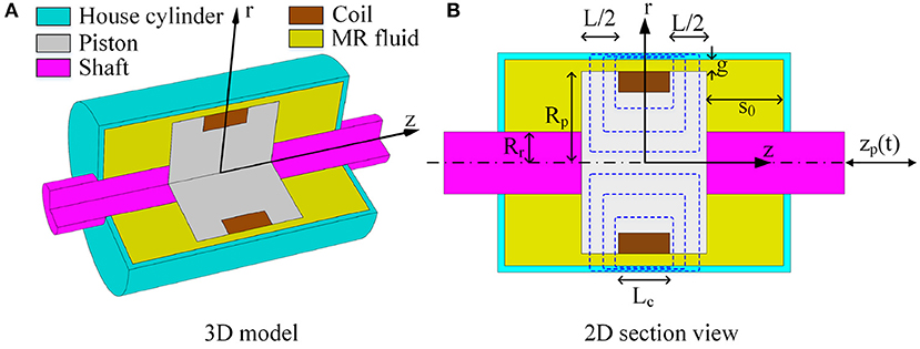
Figure 1. Layout of the MR damper. (A) Main components. (B) Main design parameters.

The piston reciprocates inside the house cylinder filled with MR fluid. Then the MR fluid is forced to flow from one chamber to the other, through the annular gap between the cylinder and the piston. Since the structure is axisymmetric, the fluid flow in an MR damper can often be reasonably assumed to be axisymmetric too. A small electromagnet coil wound around the piston generates a magnetic field in the working gap (in the r direction) which is perpendicular to the fluid flow (mainly in the z direction). The magnetic field causes iron particles in the MR fluid to form linear chains parallel to the field. This phenomenon solidifies the suspended iron particles and restricts the fluid movement. Consequently, the yield strength which can be adjusted by controlling input currents is developed within the fluid. The aim of a mechanical model is to predict the damping force under various input currents and piston movements.

Governing Equations for Viscous Fluid in ALE Form

The governing equations for viscous fluids can be expressed in either total ALE form (both time derivatives and spatial derivatives are in the referential configuration) or updated ALE form (only time derivatives are kept in the referential form). The latter is more convenient for the finite element implementation.

The mass and momentum conservations in the updated ALE form can be derived as (Bazilevs et al., 2013; Belytschko et al., 2013)

$\begin{array}{ll}\frac{\partial \rho }{\partial t}{|}_{\chi }+\text{c}·\nabla \rho +\rho \nabla ·\text{v}=0& (1)\end{array}$

$\begin{array}{ll}{\rho \frac{\partial \text{v}}{\partial t}|}_{\chi }+\rho \text{c}·\nabla \text{v}=\nabla ·\sigma +\rho \text{g}& (2)\end{array}$

where ρ is the fluid density, the total stress tensor is $\sigma =-p\text{I}+\eta \text{D}-\frac{2}{3}\eta (\nabla ·\text{v})\text{I}$, p is the pressure, D = ∇v + (∇v)^T is the strain rate tensor, η is the viscosity of fluids, the convective velocity is defined by $\text{c}=\text{v}-\widehat{\text{v}}$. $\frac{\partial }{\partial t}{|}_{\chi }$is the ALE time derivative, that is, the partial derivative with respect to time (t) when holding the ALE coordinate (χ) fixed. As mentioned above, an axisymmetric flow is assumed in an MR damper, and the spatial coordinates (x) are denoted by (r, θ, z ), and the ALE coordinate (χ) by $(\widehat{r},\widehat{\theta },ẑ)$ throughout this study.

Since the structure is, the fluid flow in an MR damper can often be reasonably assumed to be axisymmetric too.

Constitutive Equation: Weakly Compressible Bingham Fluid

Viscoplasticity

The ability of MR fluids to reversibly change from free-flowing linear viscous fluids to semi-solid can be described by the Bingham constitutive equation in which the stress tensor is related to the velocity field by

$\begin{array}{ll}\{\begin{array}{cc}\text{D}=0\hfill & \left|\tau \right|\le {\tau }_y,\text{ pre}-\text{yield zone}\\ \tau ={\tau }_y+{\eta }_p\text{D}\hfill & \left|\tau \right|>{\tau }_y,\text{ post}-\text{yield zone}\hfill \end{array}\hfill & (3)\end{array}$

where, $\left|\text{D}\right|={\left(\frac{1}{2}\text{D}:\text{D}\right)}^{1/2}$ is the magnitude of the strain rate tensor. |τ| is the magnitude of deviatoric stress tensor τ. The post-yield viscosity η_p is assumed to be a constant, and τ_y is the shear yield strength dependent on magnetic field intensity. However, it is difficult to identify, in advance, the pre- and post- yield zones in order to apply Equation (3) to the different zones. A popular approach to overcoming this difficulty is to approximate Equation (3) by a regularized equation which is applicable throughout the material without branches. Several such regularized equations were proposed (Frigaard and Nouar, 2005), and here we adopt the one proposed by Papanastasiou (1987), as in previous studies (Syrakos et al., 2016). It is formulated as follows:

$\begin{array}{ll}\tau =\left[\frac{{\tau }_y}{\left|\text{D}\right|}\left(1-e^{-m\left|\text{D}\right|}\right)+{\eta }_p\right]\text{D}={\eta }_{MR}\text{D}& (4)\end{array}$

where m is a parameter controlling the quality of the approximation. Increasing this parameter makes Equation (4) better approximate (3), but also makes the equations stiffer and harder to solve, so a compromise has to be made. η_MR is the effective viscosity of MR fluid.

For better controllability, we construct the following flexible viscoplastic model in this study. Compared to the modified Bingham model (4), details such as the “stiction” phenomenon and the shear thinning/thickening effect are added.

$\begin{array}{ll}\tau =\frac{tanh\left(k_{\text{pre}}|\text{D}|\right)\left({\tau }_{\text{pre}}+{\tau }_{\text{pos}}\right)}{|\text{D}|}\text{D}={\eta }_{\text{MR}}\text{D}& (5)\end{array}$

where ${\tau }_{\text{pre}}=\frac{1-tanh\left[k_{\text{pos}}(|\text{D}{|}^2-w^2)\right]}{2}({\tau }_{\text{ys}}-{\tau }_{\text{yd}})$, ${\tau }_{\text{pos}}={\tau }_{\text{yd}}+k_{\text{HB}}|\text{D}{|}^{1/m_{\text{HB}}}$, k_pre, k_pos and w are the dimensionless parameters controlling the pre-yield viscosity, post-yield viscosity and the “stiction” strain range width. τ_ys (Pa) and τ_yd (Pa) are the static (or critical) and dynamic yield stress strengths of MR fluids which are analogous to static and dynamic frictions in tribology. k_HB (Pa· s) and m are fluid parameters of the well-known Herschel-Bulkley model. A typical curve of the above model in one dimension is presented in Figure S1.

Weak Compressibility

A closure condition in the form of equation of state (EOS) has to be provided to complete the problem we want to solve. For compressible liquids, the Tait equation of state is widely used in many applications and hence employed in this study. It relates the pressure to the fluid density by (Koukouvinis et al., 2017)

$\begin{array}{ll}p=B\left[{\left(\frac{\rho }{{\rho }_0}\right)}^n-1\right]+p_0& (6)\end{array}$

where B is the bulk modulus, ρ₀ is the reference density, p₀ is the reference pressure, and n is an exponent adjusting the stiffness of the fluid. Alternatively, the density can be expressed in terms of the pressure as

$\begin{array}{ll}\rho ={\left(1+\frac{p-p_0}{B}\right)}^{1/n}{\rho }_0& (7)\end{array}$

Spatial Domains and Boundary Conditions

As shown in Figure 2, the whole spatial domain (Ω) is composed of the chamber domain (Ω_C1,Ω_C2) and the working gap domain (Ω_g) so that Ω = Ω_C1⋃Ω_g⋃Ω_C2, and Ω_C1⋂Ω_g⋂Ω_C2 = ∅.

FIGURE 2

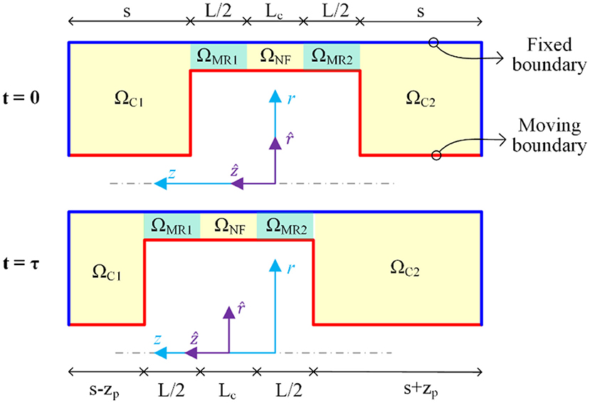
Figure 2. Fluid domains and boundary condition.

The gap domain is further divided into the subdomain right above the electromagnetic coil where no magnetic flux passes through (Ω_NF) and the subdomains themselves being parts of the magnetic circuit (Ω_MR1 and Ω_MR2). That is Ω_g = Ω_MR1⋃Ω_NF⋃Ω_MR2 and Ω_MR1⋂Ω_NF⋂Ω_MR2 = ∅.

The fluids in domains Ω_C1, Ω_C2, and Ω_NF are not exposed to the magnetic field, so they freely flow like the Newtonian fluid with constant viscosity η_p, while the fluids domains Ω_MR1 and Ω_MR2 behave like the Bingham fluid with a magnetic field dependent viscosity. Thus, these two types of fluids are distinguished from each other by their viscosities (η):

$\begin{array}{ll}\eta =\{\begin{array}{cc}{\eta }_p(r,z)& (r,z)\in {\Omega }_{\text{C}1}or{\Omega }_{\text{C}2}or{\Omega }_{\text{NF}}\\ {\eta }_{\text{MR}}(r,z)& (r,z)\in {\Omega }_{\text{MR}1}\text{ or }{\Omega }_{\text{MR}2}\\ \end{array}& (8)\end{array}$

The fluid velocities at the inner wall of the house cylinder are set to zeros, and the fluid velocities at the surface of the piston are set to the piston velocity, as shown in Figure 2. Initially, the piston is located midway along the cylinder and the MR fluid is at rest.

Mesh Updating Equation

The fluid domain varies with time due to the piston movement. Mesh updating is necessary to track the moving boundaries as well as to avoid the severe distortions of elements. For simplicity, the mesh points are allowed to move only in the axial direction when taking account of the physical domain changes. The mesh motion on the gap domain is simply a rigid translation along the axial direction, i.e.,

$\begin{array}{ll}z(\widehat{z},t)=\widehat{z}+z_p,\widehat{z}\in {\Omega }_{\text{g}}& (9)\end{array}$

where z_p = z₀ sin (2πft) is the piston displacement, z₀ is the amplitude, f is the excitation frequency.

A linear interpolation strategy is used to describe the motions of mesh nodes in the chambers, such that the displacements at the left and right piston ends (ẑ_L1 = −(L + L_c)/2 and ẑ_R1 = (L + L_c)/2 in Figure 2) is equal to the piston velocity and the displacements at the left and right fixed cylinder ends (ẑ_L0 = −(L + L_c + 2s)/2, ẑ_R0 = (L + L_c + 2s)/2 in Figure 2) are zeros. The mesh motions for the left (Ω_C1) and right chambers (Ω_C2) are

$\begin{array}{ll}z(\widehat{z},t)=\{\begin{array}{cc}(\widehat{z}+z_{0}sin(2\pi ft))\frac{\widehat{z}-{\widehat{z}}_{L0}}{{\widehat{z}}_{L1}-{\widehat{z}}_{L0}}& \widehat{z}\in {\Omega }_{\text{C}1}\\ (\widehat{z}+z_{0}sin(2\pi ft))\frac{\widehat{z}-{\widehat{z}}_{R0}}{{\widehat{z}}_{R1}-{\widehat{z}}_{R0}}& \widehat{z}\in {\Omega }_{\text{C}2}\\ \end{array}& (\mathrm{10.a})\end{array}$

The mesh nodes are fixed in the radial direction, that is, their spatial positions of are kept unchanged

$\begin{array}{ll}r\left(\widehat{r},t\right)=\widehat{r},\widehat{r}\in {\Omega }_{\text{C}1}\cup {\Omega }_{\text{C}2}& (11)\end{array}$

Finite Element Formulations

Weak Forms

In order to apply the finite element method (FEM) to the problem, all of the above differential equations should be transformed into equivalent weak forms. This transformation can be formulated in different manners. Here, the Galerkin method is applied to the continuity equation, while the consistent streamline upwind Petrov-Galerkin (SUPG) formulation is used for the momentum equation (Huerta and Liu, 1988). Triangular elements of continuous linear velocity and pressure are used for the spatial discretization of the integral equations.

The weak form of the continuity equation is obtained by multiplying the strong form (1) by the pressure test function δp and integrating over the current spatial domain (Ω):

$\begin{array}{ll}{\displaystyle {\int }_{\Omega }}\delta p\left(\frac{\partial \rho }{\partial t}{|}_{\chi }+\text{c}·\nabla \rho +\rho \nabla ·\text{v}\right)d\Omega =0& (12)\end{array}$

Another equivalent weak form of continuity, which is expressed in terms of pressure, can be obtained by using Equation (7). Firstly, a straightforward differentiation gives the relationship between the material time derivatives of fluid density and pressure as

$\begin{array}{ll}\stackrel{\bullet }{\rho }=\frac{{\rho }_0}{\beta }\stackrel{\bullet }{p}& (13)\end{array}$

where $\beta =Bn{\left(1+\frac{p-p_0}{B}\right)}^{1-1/n}$.

Then making use of Equations (7, 13), the mass Equation (1) is rewritten as

$\begin{array}{ll}\stackrel{\bullet }{p}+\beta {\left(1+\frac{p-p_0}{B}\right)}^{1/n}\nabla ·\text{v}=0& (14)\end{array}$

If n = 1, the above equation is reduced to the simpler form

$\begin{array}{ll}\stackrel{\bullet }{p}+\left(B+p-p_0\right)\nabla ·\text{v}=0& (15)\end{array}$

Furthermore, if only a perturbation of the incompressible state is of interest (i.e., the cases for which |p − p₀|/B ≪ 1), the above equation is simplified to the more familiar form (Phelan et al., 1989)

$\begin{array}{ll}\stackrel{\bullet }{p}+B\nabla ·\text{v}=0& (16)\end{array}$

Finally, an alternative weak form of the continuity equation is obtained as

$\begin{array}{ll}{\displaystyle {\int }_{\Omega }}\delta p\left[\frac{\partial p}{\partial t}{|}_{\chi }+\text{c}·\nabla p+\beta {\left(1+\frac{p-p_0}{B}\right)}^{1/n}\nabla ·\text{v}\right]d\Omega =0& (17)\end{array}$

This equation will be used in the following development of finite element implementation.

In the SUPG method, the velocity test function, $\delta \tilde{\text{v}}$, is the sum of two terms, i.e., $\delta \tilde{\text{v}}=\delta \text{v}+\delta {\text{v}}^{\text{pg}}$. The first term, δv, is continuous within the elements and across their boundaries and the second term, δv^pg, is the discontinuous streamline contribution. Moreover, δv^pg is given by (Belytschko et al., 2013)

$\begin{array}{ll}\delta {\text{v}}^{\text{pg}}={\tau }_m\text{c}·\nabla \delta \text{v}& (18)\end{array}$

where the stabilization parameter τ_m is chosen to be (Tezduyar et al., 1992)

$\begin{array}{ll}{\tau }_m={\left[{\left(\frac{2}{\Delta t}\right)}^2+{\left(\frac{2\left|{\text{v}}^h\right|}{h}\right)}^2+{\left(\frac{4\upsilon }{h^2}\right)}^2\right]}^{-1/2}& (19)\end{array}$

where t is the time-step size, $\left|{\text{v}}^h\right|=\sqrt{{\left(v_r^h\right)}^2+{\left(v_z^h\right)}^2}$ is the velocity norm, h is the element length and $\upsilon =\frac{\eta }{\rho }$ is the kinematic viscosity.

Multiplying Equation (2) by the velocity test function $\delta \tilde{\text{v}}$ and then integrating over the current spatial domain yields the weak form of the momentum equation:

$\begin{array}{l}{\displaystyle {\int }_{\Omega }}\delta \text{v}·\left(\rho \frac{\partial \text{v}}{\partial t}{|}_{\chi }+\rho \text{c}·\nabla \text{v}-\nabla ·\sigma \right)d\Omega \\ +{\displaystyle {\int }_{\Omega }}\delta {\text{v}}^{\text{pg}}·\left(\rho \frac{\partial \text{v}}{\partial t}{|}_{\chi }+\rho \text{c}·\nabla \text{v}-\nabla ·\sigma \right)d\Omega =0& (20)\end{array}$

where δv vanishes on essential boundaries (where the flow velocity is imposed). The first term of the above equation is the standard Galerkin terms while the last term serves as a stabilization term.

Matrix Equations

The continuous element shape functions for the velocity and pressure at node “I” are, respectively, N_I, $N_I^p$.

Continuity Equation

The pressure and its test function are, respectively, approximated by

$\begin{array}{ll}p=p_J(t)N_J^p& (21)\end{array}$

$\begin{array}{ll}\delta p=\delta p_I(t)N_I^p& (22)\end{array}$

Then the spatial discretization of the weak form of the continuity equation, Equation (13), gives

$\begin{array}{ll}{\text{M}}^p{\frac{\partial \text{p}}{\partial t}|}_{\chi }+{\text{L}}^p\text{p}+\text{Gv}=0& (23)\end{array}$

where the nodal pressure vector is

$\begin{array}{ll}\text{p}=\left[p_J\right]& (24)\end{array}$

and its ALE time derivative is

$\begin{array}{ll}\frac{\partial \text{p}}{\partial t}{|}_{\chi }=\left[\frac{\partial p_J}{\partial t}{|}_{\chi }\right]& (25)\end{array}$

the flow velocity vector is

$\begin{array}{ll}\text{v}=\left[v_{iJ}\right]& (26)\end{array}$

the mass matrix is

$\begin{array}{ll}{\text{M}}^p={\displaystyle \sum _e}\left[{\displaystyle {\int }_{{\Omega }^e}}{N}_I^p{N}_J^{p}d\Omega \right]& (27)\end{array}$

the matrix L^p is

$\begin{array}{ll}{\text{L}}^p={\displaystyle \sum _e}\left[{\displaystyle {\int }_{{\Omega }^e}}{N}_I^p{c}_i{N}_{J,i}^{p}d\Omega \right]& (28)\end{array}$

the matrix G is

$\begin{array}{ll}\text{G}={\displaystyle \sum _e}\left[{\displaystyle {\int }_{{\Omega }^e}}{N}_I^p\beta {\left(1+\frac{p-p_0}{B}\right)}^{\frac{1}{n}}{N}_{J,i}d\Omega \right]& (29)\end{array}$

In the above notations used in the formulations of matrix equations, lowercase subscripts are used for components, and uppercase subscripts for nodal values. Square brackets denote matrix notation of tensors. The sum over elements is interpreted as the assembling of the element contributions.

Momentum Equation

The velocity is approximated by

$\begin{array}{ll}{v}_i=v_{iJ}{N}_J& (30)\end{array}$

The velocity test function is discretized as

$\begin{array}{ll}{\delta ṽ}_i=\delta v_i+\delta v_i^{PG}& (31)\end{array}$

where δv_i = δv_iIN_I and $\delta v_i^{PG}=\tau c_j\delta v_{iI}{N}_{I,j}$, and it is equivalent to

$\begin{array}{ll}{\delta ṽ}_i=\delta v_{iI}{Ñ}_I& (32)\end{array}$

where Ñ_I = N_I + τ c_jN_{I, j}.

Substituting discretizations of velocity and its test function (Equations 30–32) into the weak form of momentum equation (Equation 20) yields

$\begin{array}{ll}\left(\text{M}+{\text{M}}_{\text{stab}}\right)\frac{\partial \text{v}}{\partial t}{|}_{\chi }+\left(\text{L}+{\text{L}}_{\text{stab}}\right)\text{v}+\left({\text{f}}^{\text{int}}+{\text{f}}_{\text{stab}}^{\text{int}}\right)=\left({\text{f}}^{\text{ext}}+{\text{f}}_{\text{stab}}^{\text{ext}}\right)& (33)\end{array}$

where the material velocity vector is v and its ALE time derivative is

$\begin{array}{ll}\frac{\partial \text{v}}{\partial t}{|}_{\chi }=\left[\frac{\partial v_{iJ}}{\partial t}{|}_{\chi }\right]& (34)\end{array}$

the mass matrices are

$\begin{array}{llll}\text{M}& =& {\displaystyle \sum _e}\left[{\displaystyle {\int }_{{\Omega }^e}}\rho N_{I,j}{N}_{J}d\Omega \right]& (35)\end{array}$

$\begin{array}{llll}{\text{M}}_{\text{stab}}& =& {\displaystyle \sum _e}\left[{\displaystyle {\int }_{{\Omega }^e}}\rho \tau c_j{N}_{I,j}{N}_{J}d\Omega \right]& (36)\end{array}$

the viscosity matrices are

$\begin{array}{llll}\text{L}& =& {\displaystyle \sum _e}\left[{\displaystyle {\int }_{{\Omega }^e}}{N}_I\rho c_j{N}_{J,j}d\Omega \right]& (37)\end{array}$

$\begin{array}{llll}{\text{L}}^{\text{stab}}& =& {\displaystyle \sum _e}\left[{\displaystyle {\int }_{{\Omega }^e}}\rho \tau c_j{N}_{I,j}{c}_k{N}_{J,k}d\Omega \right]& (38)\end{array}$

the internal force matrices are

$\begin{array}{llll}{\text{f}}^{\text{int}}& =& -{\displaystyle \sum _e}\left[{\displaystyle {\int }_{{\Omega }^e}}{N}_I{\sigma }_{ji,j}d\Omega \right]& (39)\end{array}$

$\begin{array}{llll}{\text{f}}_{\text{stab}}^{\text{int}}& =& -{\displaystyle \sum _e}\left[{\displaystyle {\int }_{{\Omega }^e}}\tau c_j{N}_{I,j}{\sigma }_{ki,k}d\Omega \right]& (40)\end{array}$

the external force matrices are

$\begin{array}{llll}{\text{f}}^{\text{ext}}& =& {\displaystyle \sum _e}\left[{\displaystyle {\int }_{{\Omega }^e}}{N}_I\rho b_{i}d\Omega \right]& (41)\end{array}$

$\begin{array}{llll}{\text{f}}_{\text{stab}}^{\text{ext}}& =& {\displaystyle \sum _e}\left[{\displaystyle {\int }_{{\Omega }^e}}\tau c_j{N}_{I,j}\rho b_{i}d\Omega \right]& (42)\end{array}$

Finally, the velocity and pressure fields are obtained by numerically solving these non-linear ordinary differential equations. Then the damping force of the MR damper, F_L, can be calculated by integrating the total stress along the moving piston boundary in Figure 2

$\begin{array}{ll}{F}_L={\displaystyle {\int }_{R_r}^{R_p}}\sigma ·{\widehat{\text{n}}}_{z}d\widehat{\Gamma }& (43)\end{array}$

where $d\widehat{\Gamma }$ is the differential line element of the piston surface with the outward unit normal vector ${\widehat{\text{n}}}_z$ in the z-direction. In addition to the force that fluid acts on the piston, the measured forces include the inertial force of the piston, so the final damping force should be calculated as

$\begin{array}{ll}F=F_L+F_m& (44)\end{array}$

where the inertial force is F_m = m_pa_p, m_p is the total mass of the piston and connectors, a_p is the acceleration of the piston.

Implementations of Weak Form PDEs in a General FEM Program

The above SUPG based FEM model was implemented in the general-purpose FEM program software Comsol Multiphysics (Version, 5.0a) which provides an efficient computational platform to solve various types of PDEs (COMSOL Inc., 2014). Three weak-form PDE modules were used, respectively, for the continuity equation (variable: pressure), momentum equation (variables: flow velocities), and the constitutive equation (variables: viscous stress). Heavy use was made of Comsol's scalar expressions (for example, expressions for the total stress components) in order to keep the whole model organized. The built-in for element length allows the stabilization terms to be implemented easily.

Owing to the strong nonlinearity of the problem, small time steps and tight absolute solver tolerances (10⁻⁵ for the flow velocities, 10⁻³ for the pressure and viscous stresses) were adopted. The implicit the backward differentiation formula (BDF) solver with the second order of accuracy was used to discretize model PDEs in time. The resulted system of non-linear algebraic equations was solved using the Newton-Raphson algorithm. We then took advantage of the efficient built-in direct solver “MUMPS” solver (MUltifrontal Massively Parallel Sparse direct Solver) to solve the system of linear equations. The calculation of the damping force in Equation (43) was implemented in Comsol as a boundary coupling operator.

Parametric Study on Inertial-Viscous-Frictional-Elastic Transients

In this section, we take an overall picture of the coupled inertial-viscous-frictional-elastic transients, by conducting a parametric analysis for an MR damper which will be experimentally study later. The structural parameters of this damper and the material properties of the MR fluid are shown in Table 1. The damper will be excited by a medium-frequency sinusoidal displacement (8 mm, 10 Hz), and the low- and high- frequency loading cases will be included in later sections. For each parametric analysis, only one dominant parameter is changed by three levels while keeping the other parameters fixed.

TABLE 1

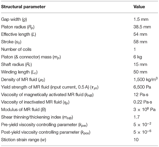
Table 1. Main design parameters of MR damper and material properties of MR fluid.

The inertial effect becomes more significant with larger fluid densities. When increasing the fluid density, larger fluctuations in the damping force appear when the damper enters the post-yield zone, as shown in Figure 3. Meanwhile, the displacement-force loop in Figure 3A rotates clockwise. It is reasonable to expect that under a frequency excitation frequency these inertia related effects will be further enhanced, and this will be seen in later sections.

FIGURE 3

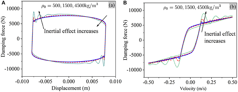
Figure 3. The inertial effect in MR dampers. (A) Displacement-force loop. (B) Velocity-force loop.

When increasing the viscosity (k_HB), the damping force increases apparently and the shape of the displacement-force loop becomes more elliptic, as shown in Figure 4.

FIGURE 4

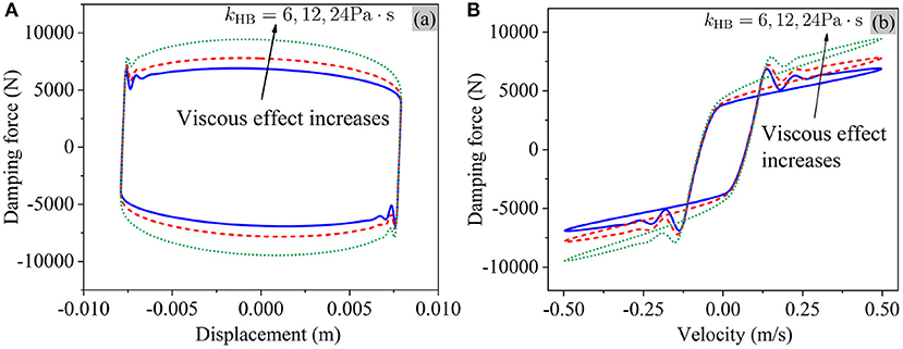
Figure 4. The viscous effect in MR dampers. (A) Displacement-force loop. (B) Velocity-force loop.

Figure 5 shows the “frictional” effect which is perhaps the most salient feature of MR dampers. The damping force is strongly in proportion to the shear yield strength of MR fluids which can be continuously adjusted by controlling the input currents.

FIGURE 5

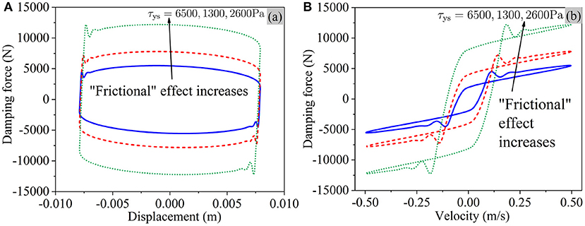
Figure 5. The “frictional” effect in MR dampers. (A) Displacement-force loop. (B) Velocity-force loop.

The elastic effect due to the compressibility of MR fluids, which has been neglected in most previous computational fluid studies on MR dampers, however, has a great impact on the performance of an MR damper.

Because of the compressibility of MR fluid, the damping force cannot change instantly but gradually varies when the piston reversing its direction as shown in Figure 6A, and this leads to an obvious velocity-force hysteresis loop in the pre-yield region as shown in Figure 6B.

FIGURE 6

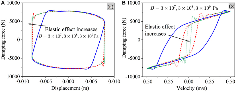
Figure 6. Elastic effect in MR dampers. (A) Displacement-force loop. (B) Velocity-force loop.

Experiment

After having a basic overview of coupled inertial-viscous-frictional-elastic transients in MR dampers, an experimental study will be performed to validate the FEM model. The performance of an MR damper (Zhixing S & T Ltd., Jiangsu, China) was tested on a hydraulic universal testing machine, with the experimental test setup shown in Figure 7. The main design parameters of the damper were listed in Table 1, and the material properties of MR fluids are also shown in Table 1.

FIGURE 7

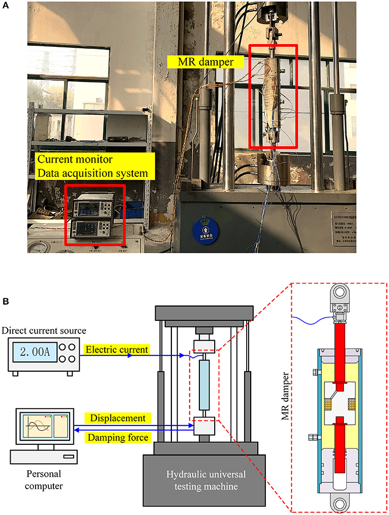
Figure 7. Experimental setup. (A) Picture of the experimental setup. (B) Schematic diagram of experiment.

A DC current source was used to apply electric currents to the damper. The damping forces were tested under the low-, medium and high- frequency sinusoidal displacement excitations: 40 mm/2 Hz, 8 mm/10 Hz, 5 mm/20 Hz. To ensure that the dissipation heating is not too high, the temperatures at typical positions was measured by thermocouples connected to a data acquisition system.

For confirming the applied input currents, a digital multimeter was used to monitor in real time the input currents. It was found that the temperature nearly remained unchanged due to the short testing time, and that the DC current source output was accurate. Supplied by the manufacture (Zhixing S & T Ltd., Jiangsu, China), the shear yield strength at typical input currents of 0.5 and 1 A are, respectively, 6,500 and 13,000 Pa. According to previous work by Guo et al. (2014), the equivalent shear yield strength without input current can be calculated from the frictional force (483 N) as 17,000 Pa.

Mesh Sensitivity Examination

Before validating the FEM model by using the experimental data, it is necessary to study the effect of mesh dependency of the model results. Three refinement levels, i.e., coarse, normal, and fine meshes with 5,473, 13,075, and 26,734 degrees of freedom (DOFs), respectively (Figure S2), were used to simulate the performance of the MR damper under the medium-frequency sinusoidal displacement excitation. As shown in Figure S3, the difference between the model results is negligible (in terms of either displacement-force or velocity-force loop), and we will choose the normal mesh in the following validation of the model. It is worth pointing out that about 2 days were used to solve the model with the fine mesh on a personal computer (i7 CPU, 8G RAM), while the models with the coarse and normal meshes only took several hours.

Validation of the FEM Model

The performance of the tested MR damper in previous section is simulated in this section. As shown in Figures 8–10, the overall agreement is good between the model predictions and the experimental data.

FIGURE 8

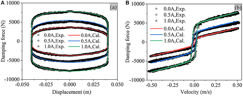
Figure 8. Performance of MR damper under low-frequency excitations (40 mm/² Hz, symbols: experimental data; lines: FEM predictions). (A) Displacement-force loop. (B) Velocity-force loop.

FIGURE 9

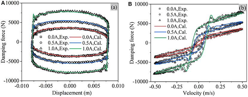
Figure 9. Performance of MR damper under medium-frequency excitations (8 mm/10 Hz, symbols: experimental data; lines: FEM predictions). (A) Displacement-force loop. (B) Velocity-force loop.

FIGURE 10

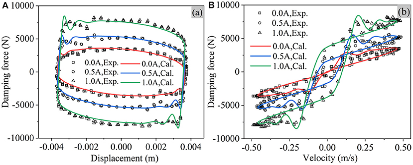
Figure 10. Performance of MR damper under high-frequency excitations (4 mm/20 Hz, symbols: experimental data; lines: FEM predictions). (A) Displacement-force loop. (B) Velocity-force loop.

The hysteretic behavior of MR dampers, either in terms of the force-displacement or the force-velocity, is frequency dependent. With increasing excitation frequency, the force-displacement loop rotates because of the larger inertial effect. The damping force oscillates more violently under the high frequency excitation. With increasing excitation frequency, the force-velocity loop in the pre-yield grows fatter and the loop in the post-yield is no longer ignorable. It is interesting to note that force oscillation is observed when the MR damper switches from the pre-yield region to the post-yield region, and it is very similar to the classical step response for a mas-spring-damper second order system. Although similar results were achieved in the previous studies on lumped parameter modeling of MR dampers (Nguyen and Choi, 2009; Gołdasz and Sapinski, 2013), few attempts have been made to explain such step-response-like force variation. Detailed explanation well be made later in this study in terms of mass the flow rates.

The discrepancy between the experimental and calculated results, which becomes more apparent under high frequency-excitations, is still not clear and worth further studying in future works. However, we believe that a more realistic modeling the compressibility of MR fluid should enhance the accuracy of the FEM model.

Discussion and Future Works

Flow Field Within Damper

The FEM model makes it possible to have a clear picture of the flow of MR fluid in an MR damper. As shown in Figure 11, the flow velocity magnitude during one complete high-frequency excitation cycle is presented at typical time instants (0, T/4, 2T/4, 3T/4, T; T = 0.05s is the excitation period).

FIGURE 11

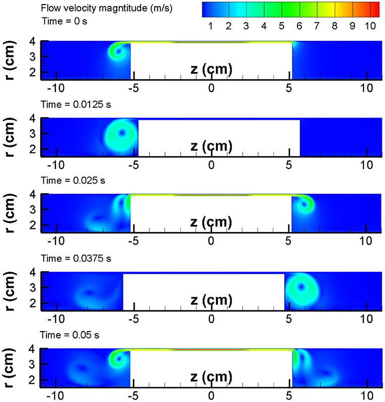
Figure 11. Snapshots of the flow field (Sinusoidal displacement excitation: 8 mm/10 Hz, 0.5 A).

The high-speed flow of MR fluid mainly happens in the working gap as expected. The mean velocities throughout the gap [including both unenergized zone (Ω_NF) and the energized zones (Ω_MR1 and Ω_MR2)] should be roughly equal, in order to satisfy continuity. However, in the energized section, due to the yield stress, the velocity profile is more plug-like, i.e., flatter and this can be seen clearly in Figure S4.

The velocity profile in the unenergized sections is more pointed. Therefore, in the unenergized section, the maximum velocity is higher, but in the energized sections the velocity is closer to the piston velocity. The overall flow rates should be roughly equal in both energized and unenergized sections. When the piston reversing its direction (t = T/4, 3T/4), a large vortex is observed near the gap end, and the fluid elsewhere moves slowly in the chamber.

Mass Flow Rate

The mass flow rate in the working gap directly determines the damping force of an MR damper. In the following, let's examine the mass flow rates under different frequency loadings. The normalized flow rates at three key locations as shown in Figure 12, i.e., the left piston end (Q_P), the left (Q_L) and right (Q_R) working gap ends, are computed using boundary integral operators and then compared in Figure 13A.

FIGURE 12

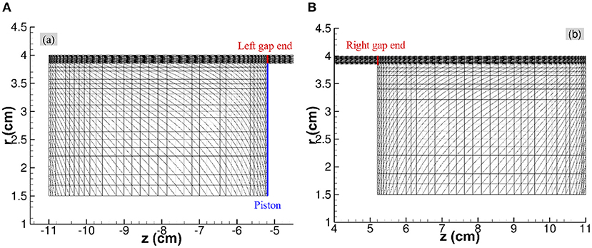
Figure 12. Key locations [left piston end (Q_P), left (Q_L), and right (Q_R) gap ends] where mass flow rates will be calculated and compared. (A) Left piston end and left gap end. (B) Right gap end.

FIGURE 13

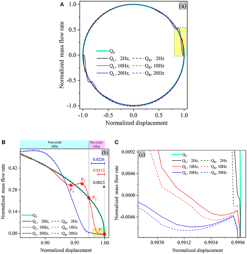
Figure 13. Normalized mass flow rate against normalized piston displacement (0.5 A). (A) Normalized displacement-mass flow rate loop. (B) Details on yellow highlight zone in (A,C). Details on yellow highlight zone in (B).

Near the maximum displacement, the flow rates at the left and right piston ends (Q_L and right Q_R) are negligibly different (as shown in Figures 13B,C), but they are apparently distinguishable from the flow rate at the piston end (Q_P). This implies that the compression of MR fluid mainly happens in the chambers rather than in the working gap.

As in the history of damping force (Figures 11–13), the similar step-response like oscillations are also observed in the mass flow rate as shown in Figure 13A. To reveal such oscillations, let's take a close view on the process when the piston changing its direction (yellow highlight zone in Figure 13A). For simplicity, we will focus the fluids in the pressurized chamber and the working gap. Several key points (P₁~P₄) in Figure 13B) split this process into different periods as below.

(1) P₁~P₂ period: In this period, the MR damper works in the pre-yield zone. After changing its direction (at P₁ moment), the piston moves slowly and the fluid in the working gap is almost locked due to the large pre-yield viscosity (or the friction effect). Meanwhile, the fluid in the pressurized chamber is constantly being compressed and the pressure inside increases with the piston movement. This process continues up to P₂ moment when the accumulated pressure in the chamber become large enough to balance the friction force in the working gap. The nonzero flow rate in this (pre-yield) period is because we have used in our FEM model a very large but finite pre-yield viscosity instead of an infinitely large one as in the ideal Herschel-Bulkley model, and the fluid can flow very slowly even in the pre-yield zone.

(2) P₂-P₃ period: After P₂ moment, the damper enters the post-yield zone. Because the post-yield viscosity is several orders lower than the pre-yield viscosity, the fluid in the working gap finally can move much more freely from now on. Under the thrust of the large chamber pressure accumulated in the P₁~P₂ period, the fluid in the working gap suddenly flows “freely” at a large acceleration. At this time instant, the inertial effect becomes dominant, as evidenced by the peak in the flow rate (Point P₃ in Figure 13B) or the overshoot in the damping force.

(3) P₃-P₄ period: Much like the case of a small extending instantly applied to a pre-compressed spring, when the fluid in the chamber suddenly starts to flow outward, the pressure inside drops slightly, and the flow rate in the working gap as well as the damping force decreases accordingly. Consequently, a small undershoot (P4 in figure) appears for the first time in the post-yield zone.

(4) From P₄ to the next piston reversing moment: After the damper enters the post-yield zone, it becomes hard for the piston to squeeze the chamber fluid as it does in the pre-yield zone. Conceptually, just like it is difficult to compress a spring at an end when the other end can move. The increase in the damping force mainly is contributed by the increase in the piston velocity which leads to an increasing viscous damping force (due to the viscous effect).

If we look very closely at the mass flow rates at the two ends of the working gap, we can find small difference between them as shown in Figure 13C). Such difference results from the compressibility of MR fluid in the working gap, and it is expected to become larger with the increasing volume of the gap.

Keeping in our mind the above picture of transition of MR fluid from the pre-yield to the post-yield zone, we can actually give a reasonable estimation on the amount of the fluid compression during the pre-yield period. According to the simple Bingham fluid model, the chamber pressure (p_y) at the yield moment (P₂ in Figure 13B) can be approximated by

$\begin{array}{ll}{p}_y=2{\tau }_y\frac{L}{g}& (45)\end{array}$

Under this pressure, the piston displacement variation (or the fluid compression along the axial direction of the damper), Δz, can then be calculated from

$\begin{array}{ll}{p}_y=B\frac{dV}{V}=B\frac{\Delta zA}{(s_0-\Delta z)A}=B\frac{\Delta z}{s_0-\Delta z}& (46)\end{array}$

Where the distance of the piston away from its maximum displacement position $\Delta z=z_{0}sin(2\pi ft)-z_{0}sin\left(2\pi f\frac{T}{4}\right),\frac{T}{4}<t<\frac{T}{2}$. The meanings and values of other variables in equations (45) and (46) can be found in Table 1.

The normalized compression $\left(\frac{\Delta z}{z_0}\right)$ obtained using the Equations (45, 46) are presented in Figure 13B, and they can be used as reasonable approximations of the total fluid compression accumulated in the pre-yield zone. Moreover, the piston velocity at the yield point can also be estimated by using Equations (45, 46), and they indeed offer a good estimation on the width of the pre-yield zone (about twice the piston velocity at the yield point), as shown in Figure 14. In other words, the frictional effect and the elastic effect of MR fluid together dominate the pre-yield hysteretic behavior of MR dampers. If a small pre-yield loop is desired, the chamber volume should be as small as possible and a MR damper should work under a low input excitation current.

FIGURE 14

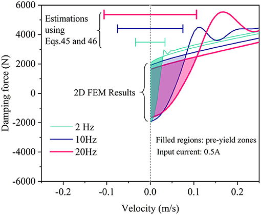
Figure 14. Width of pre-yield zone under different frequency loadings.

Compared to the previous CFD modeling studies of MR dampers, the main contribution of this study includes two aspects: (a) the compressibility of MR fluids, which has been neglected in previous studies, is proven to be essential for accurate predictions of hysteretic behavior of MR dampers; (b) the mechanism behind the step-response-like force oscillation of an MR damper, which has been rarely reported in previous researches, is explained in detail in this study.

It is interesting to note that the hysteretic behavior of an MR damper can be described either by an incompressible viscoelastic fluid as shown in recent studies or by a compressible viscoplastic fluid as demonstrated in this work. Thus, the combination of these two constitutive models, that is, a compressible viscous-elastic-plastic fluid model, is believed to predict the hysteretic behavior of MR dampers more accurately, and this will be investigated in our future works.

Conclusion

In this paper, the coupled inertial-viscous-frictional-elastic transients in MR dampers was investigated using finite element simulation and experimental validation under low-, medium-, and high- frequency sinusoidal displacement excitations and different input electric currents. The main concluding points are as follows:

(1) Representing the piston movements by the moving boundaries, the ALE form of the conservation laws offers a natural way to describe the fluid flow in MR dampers. The flow problem in MR dampers can be effectively solved by the SUPG based FEM method and the solution exhibits little mesh-size sensitivity.

(2) The weak compressibility of MR fluids is crucial to accurately predict and understand the dynamic performances of MR dampers. It should not be ignored, as in most previous studies on modeling of MR devices. The compression of fluids mainly happens in the pressurized chamber instead of the working gap, and it can be reasonably estimated on the basis of the shear yield strength and bulk modulus of MR fluid.

(3) The mechanical model of MR dampers is essentially a second order mass-spring-viscous (friction) model. The widely used Bouc-Wen model is intrinsically deficient for accurate predictions, because it is only a first order system. In the second order system of MR dampers, the fluid density reflects the inertial effect, as indicated by the fatness of the hysteretic loop in the post-yield zone. The post-yield viscosity controls the proportion between the damping force and the piston velocity in the post-yield zone. The shear yield strength gives rise to the fictional effect and governs the magnitude of damping force in the post-yield zone. The compressibility of fluids, playing the role of a spring, is responsible for both the hysteretic loop in the pre-yield zone and the force fluctuations in the poste yield zone.

(4) The ratio of shear yield strength to the bulk modulus (τ_y/B) determines the boundary between the pre- and post-yield zones. When a MR damper crosses this boundary, a step response is observed as in a second order mass-spring-viscous system model, and it can be explained in terms of mass flow rate.

(5) The hysteretic behavior of MR dampers shows a strong dependence on the excitation frequency. With the same maximum piston velocity, both pre-yield and post-yield hysteric loops grow apparently fatter with increasing sinusoidal excitation frequency. Moreover, the damping force oscillation becomes more violent under higher frequency excitations and it becomes significant under low input currents.

To the best of our knowledge, this is the first compressible fluid based 2D flow simulation and experimental validation of coupled inertial-viscous-frictional-elastic transients in MR dampers, and it can be a valuable aid in research on general MR devices.

Data Availability Statement

The datasets generated for this study are available on request to the corresponding author.

Author Contributions

PG fully controls and performs the FEM modeling, and scientific writings. JX designs experiments and data processing. YH performs the parameter modeling of MR damper under random displacement excitation. XD guides the whole logic of this study, from modeling to experiments and to writing.

Funding

This research was supported by National Natural Science Foundation of China (No. 51308450), Research Foundation of Xi'an University of Architecture and Technology (No. RC1368), National Key R&D Program of China (2018YFC0705603), and Jiangxi Province Science Foundation for Youths (No. 20171BAB216041).

Conflict of Interest

The authors declare that the research was conducted in the absence of any commercial or financial relationships that could be construed as a potential conflict of interest.

Supplementary Material

The Supplementary Material for this article can be found online at: https://www.frontiersin.org/articles/10.3389/fmats.2019.00293/full#supplementary-material

References

Alghamdi, A. A., Lostado, R., and Olabi, A.-G. (2014). “Magneto-rheological fluid technology,” in Modern Mechanical Engineering, ed D. J. Paulo (Berlin; Heidelberg: Springer), 43–62. doi: 10.1007/978-3-642-45176-8_3

CrossRef Full Text | Google Scholar

Bazilevs, Y., Takizawa, K., and Tezduyar, T. E. (2013). Computational Fluid-Structure Interaction: Methods and Applications. John Wiley & Sons. doi: 10.1002/9781118483565

CrossRef Full Text | Google Scholar

Belytschko, T., Liu, W. K., Moran, B., and Elkhodary, K. (2013). Nonlinear Finite Elements for Continua and Structures. John Wiley & Sons.

Google Scholar

Carlson, J. D., Catanzarite, D., and St. Clair, K. (1996). Commercial magneto-rheological fluid devices. Int. J. Mod. Phys. B 10, 2857–2865. doi: 10.1142/S0217979296001306

CrossRef Full Text | Google Scholar

Case, D., Taheri, B., and Richer, E. (2016). Multiphysics modeling of magnetorheological dampers. Int. J. Multiphys. 7, 61–76. doi: 10.1260/1750-9548.7.1.61

CrossRef Full Text | Google Scholar

Chen, P., Bai, X.-X., Qian, L.-J., and Choi, S. B. (2018). An approach for hysteresis modeling based on shape function and memory mechanism. IEEE/ASME Trans. Mech. 23, 1270–1278. doi: 10.1109/TMECH.2018.2833459

CrossRef Full Text | Google Scholar

COMSOL Inc. (2014). Comsol Multiphysics User's Manual Ver. 5.0a.

Google Scholar

Frigaard, I., and Nouar, C. (2005). On the usage of viscosity regularisation methods for visco-plastic fluid flow computation. J. Nonnewton. Fluid Mech. 127, 1–26. doi: 10.1016/j.jnnfm.2005.01.003

CrossRef Full Text | Google Scholar

Gołdasz, J., and Sapinski, B. (2013). Verification of magnetorheological shock absorber models with various piston configurations. J. Intell. Mater. Syst. Struct. 24, 1846–1864. doi: 10.1177/1045389X13479684

CrossRef Full Text | Google Scholar

Gołdasz, J., and Sapinski, B. (2015). Application of CFD to modeling of squeeze mode magnetorheological dampers. Acta Mech. Autom. 9, 129–134. doi: 10.1515/ama-2015-0021

CrossRef Full Text | Google Scholar

Guo, P., Guan, X., and Ou, J. (2014). Physical modeling and design method of the hysteretic behavior of magnetorheological dampers. J. Intell. Mater. Syst. Struct. 25, 680–696. doi: 10.1177/1045389X13500576

CrossRef Full Text | Google Scholar

Guo, P., and Xie, J. (2019). Two-dimensional CFD modeling of hysteresis behavior of MR dampers. Shock Vib. 2019:9383047. doi: 10.1155/2019/9383047

CrossRef Full Text | Google Scholar

Huerta, A., and Liu, W. K. (1988). Viscous flow with large free surface motion. Comput. Methods Appl. Mech. Eng. 69, 277–324. doi: 10.1016/0045-7825(88)90044-8

CrossRef Full Text | Google Scholar

Jolly, M. R., Bender, J. W., and Carlson, J. D. (1999). Properties and applications of commercial magnetorheological fluids. J. Intell. Mater. Syst. Struct. 10, 5–13. doi: 10.1177/1045389X9901000102

CrossRef Full Text | Google Scholar

Koukouvinis, P., Mitroglou, N., Gavaises, M., and Lorenzi, M. (2017). Quantitative predictions of cavitation presence and erosion-prone locations in a high-pressure cavitation test rig. J. Fluid Mech. 819, 21–57. doi: 10.1017/jfm.2017.156

CrossRef Full Text | Google Scholar

Nguyen, Q.-H., and Choi, S.-B. (2009). A new approach for dynamic modeling of an electrorheological damper using a lumped parameter method. Smart Mater. Struct. 18:115020. doi: 10.1088/0964-1726/18/11/115020

CrossRef Full Text | Google Scholar

Papanastasiou, T. C. (1987). Flows of materials with yield. J. Rheol. 31, 385–404. doi: 10.1122/1.549926

CrossRef Full Text | Google Scholar

Phelan, F. Jr., Malone, M., and Winter, H. (1989). A purely hyperbolic model for unsteady viscoelastic flow. J. Nonnewton. Fluid Mech. 32, 197–224. doi: 10.1016/0377-0257(89)85036-0

CrossRef Full Text | Google Scholar

Sahin, H., Wang, X., and Gordaninejad, F. (2013). Magneto-rheological fluid flow through complex valve geometries. Int. J. Vehicle Des. 63, 241–255. doi: 10.1504/IJVD.2013.056154

CrossRef Full Text | Google Scholar

Sahin, I., Engin, T., and Çeşmeci, S. (2010). Comparison of some existing parametric models for magnetorheological fluid dampers. Smart Mater. Struct. 19:035012. doi: 10.1088/0964-1726/19/3/035012

CrossRef Full Text | Google Scholar

Sternberg, A., Zemp, R., and De La Llera, J. C. (2014). Multiphysics behavior of a magneto-rheological damper and experimental validation. Eng. Struct. 69, 194–205. doi: 10.1016/j.engstruct.2014.03.016

CrossRef Full Text | Google Scholar

Syrakos, A., Dimakopoulos, Y., Georgiou, G. C., and Tsamopoulos, J. (2016). Viscoplastic flow in an extrusion damper. J. Nonnewton. Fluid Mech. 232, 102–124. doi: 10.1016/j.jnnfm.2016.02.011

CrossRef Full Text | Google Scholar

Syrakos, A., Dimakopoulos, Y., and Tsamopoulos, J. (2018). Theoretical study of the flow in a fluid damper containing high viscosity silicone oil: Effects of shear-thinning and viscoelasticity. Phys. Fluids 30:030708. doi: 10.1063/1.5011755

CrossRef Full Text | Google Scholar

Tezduyar, T. E., Mittal, S., Ray, S. E., and Shih, R. (1992). Incompressible flow computations with stabilized bilinear and linear equal-order-interpolation velocity-pressure elements. Comput. Methods Appl. Mech. Eng. 95, 221–242. doi: 10.1016/0045-7825(92)90141-6

CrossRef Full Text | Google Scholar

Ursescu, A. (2005). Channel Flow of Electrorheological Fluids Under an Inhomogeneous Electric Field. Berlin: Technische Universität.

Google Scholar

Wang, D., and Liao, W. H. (2011). Magnetorheological fluid dampers: a review of parametric modelling. Smart Mater. Struct. 20:023001. doi: 10.1088/0964-1726/20/2/023001

CrossRef Full Text | Google Scholar

Yu, J., Dong, X., and Zhang, Z. (2017). A novel model of magnetorheological damper with hysteresis division. Smart Mater. Struct. 26:105042. doi: 10.1088/1361-665X/aa87d6

CrossRef Full Text | Google Scholar

Zheng, J., Yancheng, L., Zhaochun, L., and Jiong, W. (2015). Transient multi-physics analysis of a magnetorheological shock absorber with the inverse Jiles–Atherton hysteresis model. Smart Mater. Struct. 24:105024. doi: 10.1088/0964-1726/24/10/105024

CrossRef Full Text | Google Scholar

Zhou, H., and Bai, M. (2014). Three-dimensional numerical simulation of magnetorheological fluid seal technology applied on circular cooler and its experimental validation. Mech. Adv. Mater. Struct. 21, 329–340. doi: 10.1080/15376494.2013.815832

CrossRef Full Text | Google Scholar