Effects of Gradient Coil Noise and Gradient Coil Replacement on the Reproducibility of Resting State Networks

Introduction

Resting state functional magnetic resonance imaging (fMRI) is an imaging technique that does not require participants to perform any task during the scan, making the approach attractive in investigating healthy brain functions as well as in examining changes occurring in the diseased brain. Resting state fMRI is commonly used to examine functional connectivity among spatially distributed brain regions that form the so-called resting state networks (RSNs; Greicius et al., 2003; Beckmann et al., 2005; Fox et al., 2005; Damoiseaux et al., 2006). In healthy population, resting state fMRI has been proven useful in investigating the very early development of these RSNs in infancy (Fransson et al., 2007; Smyser et al., 2010) and how these RSNs are transformed across the lifespan (Tomasi and Volkow, 2012; Betzel et al., 2014; Sala-Llonch et al., 2015). In clinical population, resting state fMRI has also been used to examine changes in functional connectivity within RSNs in chronic pain conditions (Baliki et al., 2008, 2014; Martucci et al., 2015; Li et al., 2016), Parkinson’s disease (Hacker et al., 2012; Szewczyk-Krolikowski et al., 2014; Yao et al., 2014), Alzheimer’s disease (Greicius et al., 2004; Dai et al., 2015), patients with brain tumor (Esposito et al., 2012; Maesawa et al., 2015), and other neuropsychological disorders (Greicius, 2008). Using resting state fMRI, RSNs have also been shown to be highly reproducible across participants (Beckmann et al., 2005; Chen et al., 2008) and within participants over multiple sessions (Damoiseaux et al., 2006; Chen et al., 2008; Choe et al., 2015), making resting state functional connectivity a promising biomarker for clinical applications (Shimony et al., 2009; Fox and Greicius, 2010; Lee et al., 2013).

The reproducibility of RSNs, however, could be affected by several factors. One of these factors is the hardware used to acquire the imaging dataset. For multisite studies, differences in MRI providers, magnet field strengths, software and coil architectures need to be considered. Even with the same MRI scanner, maintaining the scanner’s stability throughout a given imaging study is very important in minimizing hardware-related variability in the acquired imaging dataset. For cross-sectional studies, scanner stability ensures that the variability in any MRI-derived measures is mainly due to the population being studied. For longitudinal studies, scanner stability guarantees that changes observed over time are driven by disease progression, for example, and not by instrument-related factors. However, MRI scanners do malfunction at times, which could necessitate replacement of major components such as the scanner’s gradient coil. This major change in hardware could introduce unwanted variability into the imaging dataset. Faulty MRI scanner gradient coil could also generate artifacts in the acquired images, the degree of which could vary depending on the severity of the problem. Large artifacts are easier to detect but low intensity, randomly occurring artifacts are difficult to discover. Some low intensity gradient-coil-generated noise are barely noticeable, but have the potential to significantly affect the outcome of the analysis.

In this study, we examined the effects of low intensity gradient coil noise on resting state fMRI data on the reproducibility of RSNs and introduced a method to minimize these effects. We further examined whether RSNs constructed from resting state fMRI and values of regional gray matter (GM) volume estimated from T1-weighted images are reproducible using data acquired before and after gradient coil replacement. For this, we performed voxel-wise statistical comparisons of RSNs and GM between sessions to identify differences at the voxel level. To compare RSNs, we used group independent component analysis (ICA) and dual regression analysis (Filippini et al., 2009), which have been found effective and reliable in analyzing resting state fMRI data (Zuo et al., 2010). To assess differences in GM, we used voxel-based morphometry (VBM; Ashburner and Friston, 2000), a commonly used approach for analyzing T1-weighted images. Finally, we also computed regional GM volume from several regions of interest (ROIs) and other RSN-derived metrics including within-network functional connectivity (WNFC) and similarity measures for test-retest reliability assessment.

Materials and Methods

Participants

Twenty healthy volunteers (male/female = 15/5) from Nagoya University were recruited for this study. The participants’ age ranged from 20 years to 25 years (mean = 22 years, standard deviation (SD) = 1.26 years). All participants had no history of psychiatric or neurological disorder. Participants were scanned four times, twice before (sessions S1 and S2) and twice after (sessions S3 and S4) the MR gradient coil was replaced, using the same scanning protocol. The average inter-scan interval was 67.8 days between S1 and S2, 44.0 days between S2 and S3, and 31.0 days between S3 and S4. Gradient coil noise affected some of the scans in S1 and S2 (pre-replacement) but not scans in S3 and S4 (post-replacement). The study was approved by the Ethical Committee of Nagoya University Graduate School of Medicine with approval number 1014-2. All participants signed a written informed consent before joining the study.

Magnetic Resonance Imaging

Magnetic resonance images were acquired using a Siemen’s Magnetom Verio (Siemens, Erlanger, Germany) 3.0T MRI scanner with a 32-channel head coil. For each scanning session, a T1-weighted MR image was acquired using a 3D Magnetization Prepared Rapid Acquisition Gradient Echo (MPRAGE; Siemens; Mugler and Brookeman, 1990) pulse sequence with the following imaging parameters: repetition time (TR)/MPRAGE repetition time = 7.4/2500 ms, echo time (TE) = 2.48 ms, inversion time (TI) = 900 ms, flip angle (FA) = 8 degrees, 192 sagittal slices with a distance factor of 50% and 1-mm thickness, FOV = 256 mm, acquisition matrix dimension = 256 × 256, and in-plane voxel resolution of 1.0 × 1.0 mm², with a total scan time of 5 min 49 s. Resting state functional MRI scans were also acquired using gradient echo (GE) echo planar imaging (EPI) with the following parameters: TR = 2.5 s, TE = 30 ms, 39 transverse slices with a 0.5-mm inter-slice interval and 3-mm thickness, FOV = 192 mm, matrix dimension is 64 × 64, FA = 80 degrees, 3 × 3 × 3 mm³ voxel resolution and 198 volumes. Participants were instructed to close their eyes during the scan but not to fall asleep. Other MRI scans were also acquired during the same imaging session, however the analysis of these datasets will be reported elsewhere.

Preprocessing for T1-Weighted MR Images

All images were preprocessed using SPM12 (Wellcome Trust Center for Neuroimaging, London, UK) running on Matlab R2016b (MathWorks, Natick, MA, USA). The T1-weighted images were first segmented into component images including GM, white matter (WM), cerebrospinal fluid (CSF), and other non-brain tissues using SPM12’s segmentation approach. A common template for the GM images was created using DARTEL (Diffeomorphic Anatomical Registration using Exponentiated Lie algebra; Ashburner, 2007), which was then normalized to the Montreal Neuroimaging Institute (MNI) standard space. The obtained transformation information, together with the deformation fields from DARTEL, were used to normalize the component images to MNI. The normalized images were modulated to preserve the amount of signal from each region, re-sampled to an isotropic voxel size equal to 2 × 2 × 2 mm³, and smoothed using an 8-mm full-width-at-half-maximum (FWHM) Gaussian filter. These preprocessed images were then used in the succeeding analysis.

Voxel-Based Morphometry

To compare differences between sessions at the voxel level, we used VBM, a commonly used approach for the analysis of T1-weighted images. For this, the preprocessed GM images were entered into a paired sample t-test to identify changes between sessions using SPM12. In particular, we performed S1 vs. S2 and S3 vs. S4 to compare datasets obtained using the same gradient coil as well as S1 vs. S3, S1 vs. S4, S2 vs. S3, and S2 vs. S4 to compare datasets obtained from different gradient coils. Resulting statistical maps were corrected for multiple comparisons using a family-wise error (FWE) correction rate with p < 0.05.

Reliability Assessment of Regional GM Volume

Aside from voxel-wise comparisons to assess differences between sessions in anatomical (T1) images, we also estimated other metrics for test-retest reliability assessment. These metrics were then entered into an intra-class correlation (ICC) analysis, where ICC is defined as:

$ICC(3,1)=\frac{BMS-EMS}{BMS+(k-1)EMS}$

In the above equation, BMS is the between-subject variance, EMS is the condition error variance, and k is the number of conditions (Shrout and Fleiss, 1979). ICC values range from 0 to 1, with higher values (i.e., closer to 1) indicating that the between-subject error dominates, while lower values (i.e., closer to 0) indicating that the effect of conditions dominates the error.

For this analysis, we used regional GM volumes computed from the preprocessed GM images from several ROIs defined by the AAL template (Tzourio-Mazoyer et al., 2002), which divides the whole GM into 116 ROIs. The estimated regional GM volume for each ROI from all participants and sessions were then entered into the ICC analysis.

Preprocessing for Resting State fMRI Data

For the resting state fMRI data, the first five volumes were discarded to account for the initial image inhomogeneity. The remaining images were then slice-time corrected relative to the middle slice, realigned to the mean functional image, co-registered to the bias-corrected anatomical image, normalized to MNI space using the transformation information obtained from the segmentation of the individual anatomical image, resampled to an isotropic voxel size equal to 2 × 2 × 2 mm³, and finally smoothed using an 8-mm FWHM Gaussian blurring kernel. To correct for head motion, the six estimated realignment parameters (three for translation and three for rotation), the parameters’ square, difference, and difference square were regressed out from the preprocessed data (Power et al., 2014). Mean signals from selected ROIs within WM and CSF and the global signal, plus the temporal difference of these signals, were also removed. The cleaned data were then bandpass filtered within 0.01–0.1 Hz.

Group Independent Component Analysis

Group ICA was performed using Multivariate Exploratory Linear Optimized Decomposition into Independent Components (MELODIC; Beckmann et al., 2005), a component of the FSL software package¹ to extract group-level RSNs. We used a temporal concatenation approach in MELODIC by temporally concatenating all preprocessed resting state fMRI data from all participants in all sessions. Using data from all participants and sessions in one group ICA maximizes sensitivity and avoids the problem of identifying similar components from different sessions if ICA was performed per session. We ext­racted 30 group-level independent components (ICs) to be consistent with the way the RSN templates² we used were generated (Shirer et al., 2012). These group ICs were then used in the succeeding dual regression analyses (Filippini et al., 2009).

Dual Regression Analyses

To extract participant-specific RSNs for each session, we used dual regression analysis. For each preprocessed resting state fMRI data, the identified full set of group ICs obtained from group ICA were used as spatial regressors and regression parameters were estimated at each time point giving a series of parameter estimates associated with each group IC. The estimated time courses of the regression parameters for all group ICs were then used as temporal regressors in the second regression analysis using the same resting state fMRI data to construct participant- and session-specific RSNs associated with the group RSNs. These participant-specific RSNs were then used in paired sample t-tests using nonparametric permutation testing (Nichols and Holmes, 2002) with 5000 permutations to identify regions that showed significant differences in functional connectivity. We compared RSNs generated using datasets obtained from the same gradient coil (S1 vs. S2 and S3 vs. S4) and RSNs generated using datasets from different gradient coils (S1 vs. S3, S1 vs. S4, S2 vs. S3, and S2 vs. S4). For all analyses, a threshold-free cluster enhancement technique (Smith and Nichols, 2009) was used and the resulting statistical maps were corrected for multiple comparisons by controlling FWE rate with p < 0.05.

We performed three dual regression analyses to examine the contribution of head motion and gradient coil noise in the observed differences in functional connectivity. In the first analysis, we used the bandpass filtered and cleaned resting state fMRI data from all participants without additional correction. This analysis will be referred to as the “no-correction” analysis. In the second, volumes with frame-wise displacement (FD) value greater than 0.2 were censored (scrubbing) before dual regression analysis was carried out. This analysis will be referred to as “motion-corrected” analysis. The FD value of a given volume i was calculated as FD_i = |Δx_i| + |Δy_i| + |Δz_i| + |Δα_i| + |Δβ_i| + |Δγ_i|, where Δx_i = x_(i−1) − x_i is the difference of the estimated realignment parameter (translation) along the x-axis of volumes i and (i − 1). Similarly, Δy_i, Δz_i, Δα_i, Δβ_i, and Δγ_i correspond to the other translation parameters y_i and z_i and rotation displacements α_i, β_i, and γ_i, respectively (Power et al., 2012). Rotation parameters were converted to displacements along the surface of a sphere with radius equal to 50 mm, this value being the approximate mean distance from the cerebral cortex to the center of the head. In the third analysis, referred to as “noise-corrected” analysis, we censored volumes with gradient coil noise before running dual regression analysis. An algorithm to detect the gradient coil noise is outlined in “Detection of Gradient Coil Noise” section.

Other Metrics for Reliability Assessment of RSNs

For each RSN, we also computed the mean WNFC value. To estimate WNFC, we first generated RSN-specific masks. To do this, for a given RSN, we performed a one-sample t-test using participant-specific RSN images from all participants in all sessions using SPM12. For example, to generate the mask for the dorsal default mode network (DMN), a one-sample t-test was performed using participant-specific dorsal DMN images from all participants and sessions. A threshold value equal to p < 0.0001, corrected for multiple comparisons using FWE correction, was then applied to the resulting statistical map and all voxels with p-values below the threshold were included in the mask. We used a stringent threshold value to include only voxels with very significant network connectivity. To get the value of WNFC for a given RSN, the generated mask for that RSN was then applied to the participant-specific RSN image and the mean of the voxel values within the mask was computed and assigned to WNFC. The estimated WNFC values from all participants and sessions were then entered into the ICC analysis for test-retest reliability assessments.

Aside from WNFC, we also assessed the spatial similarity of the participant-specific RSNs relative to the mean RSN image computed over all participants and sessions. We used a spatial similarity measure given by η² (Cohen et al., 2008; Choe et al., 2015):

${\eta }^2=1-\frac{{\displaystyle {\sum }_{i=1}^N{(a_i-m_i)}^2}+{(b_i-m_i)}^2}{{\displaystyle {\sum }_{i=1}^N{(a_i-\overline{M})}^2}+{(b_i-\overline{M})}^2}$

where a_i and b_i are values at voxel i in maps a and b, respectively, m_i is the mean value of the two images at voxel i, $\overline{M}$ is the grand mean across the mean image m, and N is the total number of voxels. Here, a is the participant-specific RSN and b is the mean RSN. η² values can vary from 0 to 1, with 0 indicating no similarity and 1 being identical. The main advantage of this measure is that it enables the quantification of the similarity or the difference between two images instead of just the correlation between the two images.

Detection of Gradient Coil Noise

Since gradient coil noise could randomly appear in any volume during the scan, a method to automatically detect corrupted volumes was developed. Our data showed that the gradient coil noise has: (1) low intensity, approximately 5% to 10% of the brain’s intensity; (2) affects the entire image within a slice, both within and outside the brain; and (3) randomly appears in any volume during a given scan in all or in only some slices within the image volume. An example image is shown in Figure 1. The noise is inconspicuous when using the full intensity range to display the image (Figure 1A) and becomes apparent only when the image is displayed with intensity values ranging from 10 to 50 (Figure 1B).

FIGURE 1

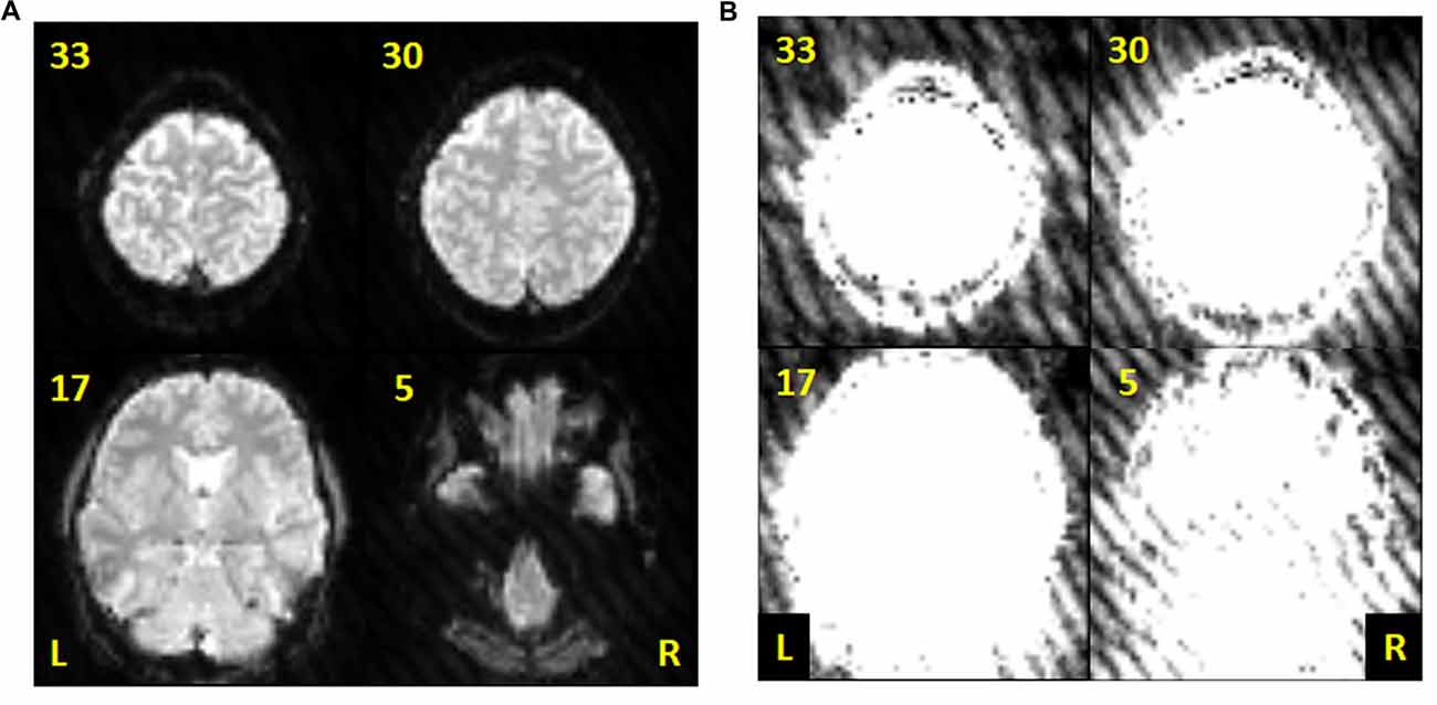
Figure 1. Sample echo planar images from the resting state data of subject 001 (volume 60). (A) Slices 5, 17, 30 and 33 displayed using intensity values ranging from 10 to 1000. (B) Same slices as in (A) but displayed using intensity values ranging from 10 to 50 to highlight the gradient coil noise throughout the image.

To detect the gradient coil noise, we used the mean intensity of the background image outside the brain. For this, we assumed the following: (1) the mean background intensity I_bg outside the brain without gradient coil noise is almost constant throughout the scan and can have different value for each slice; and (2) the mean background intensity with gradient coil noise I_noise is greater than I_bg. To estimate the mean background intensity, we generated an individualized outside-brain mask using the outside-brain component obtained from the segmentation of the anatomical image. This component was co-registered to the mean functional image to be in the same subject space as the realigned functional images.

The detection method is outlined in Figure 2. First, the mean background intensity I_m(n) for all slices and volumes was computed. The variables m and n are defined as slice and volume counters, respectively. An example of I_m(n) is shown in the top left image of Figure 2. For a given slice m (red strip in the figure), we then extracted I_m(n) (step 2.1) and estimated the difference in the mean intensity between successive volumes, that is, ΔI_m(n) = I_m(n) − I_m(n − 1) (step 2.2). Next, we identified in step 2.3 the values of n, denoted as n_p, where this difference was greater than a set threshold value thr, assumed to be the minimum jump in mean background intensity due to the gradient coil noise. This step was intended to capture sudden jumps from the background intensity I_bg, although it may also be possible that this step would capture jumps from I_noise. Next, we computed the minimum of I_m(n_p) for all n_p (step 2.4) to obtain an approximation of the minimum of I_noise. This min I_noise value is indicated by a red dash line in the figure. To estimate I_bg, we then computed the median of I_m(n) for all n where I_m(n) < min I_noise (red circles) shown as a blue dash line in step 2.5. Due to the possibility that some I_m(n) with noise would be included in the estimation of I_bg, we used the median, which is more robust to outliers, instead of the mean to minimize the potential overestimation of I_bg. The main purpose of steps 2.2–2.5 was to get an estimate of I_bg. After obtaining this estimate, we then used it to identify volumes with noisy mth slice, that is, any n satisfying I_m(n) > I_bg + thr. To do this, I_bg was subtracted from I_m(n) for each n and any n where the difference was greater than thr was labeled as “noisy” (red bars in step 2.6). This process was then repeated for other values of m. Representative result of this labeling is shown in the lower left image of Figure 2 where noisy slices are shown in yellow. Volumes with at least one slice labeled as noisy were censored in the noise-corrected analyses. In order to obtain a reasonable estimate of the individualized RSNs, participants whose remaining number of volumes after noise correction was less than 120 volumes (5 min) were excluded.

FIGURE 2

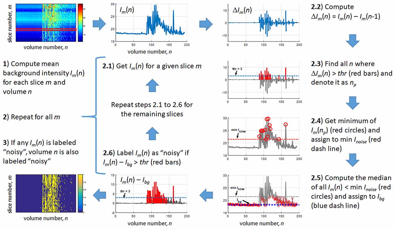
Figure 2. Outline of the proposed method for the automatic detection of gradient coil noise.

Results

Gray Matter Changes Across Sessions

All paired sample t-test comparisons of preprocessed GM images did not show any significant difference between sessions using FWE p < 0.05. Estimated ICC values for the 116 ROIs in the AAL template are plotted in Figure 3A. The mean ICC value across all ROIs was 0.96 (SD = 0.02) and ICC values ranged from 0.87 to 0.99. All values are close to 1 indicating that between-subject differences dominate compared to the differences among the four sessions. This result is reasonable as T1-weighted images appeared to be not affected by the faulty gradient coil.

FIGURE 3

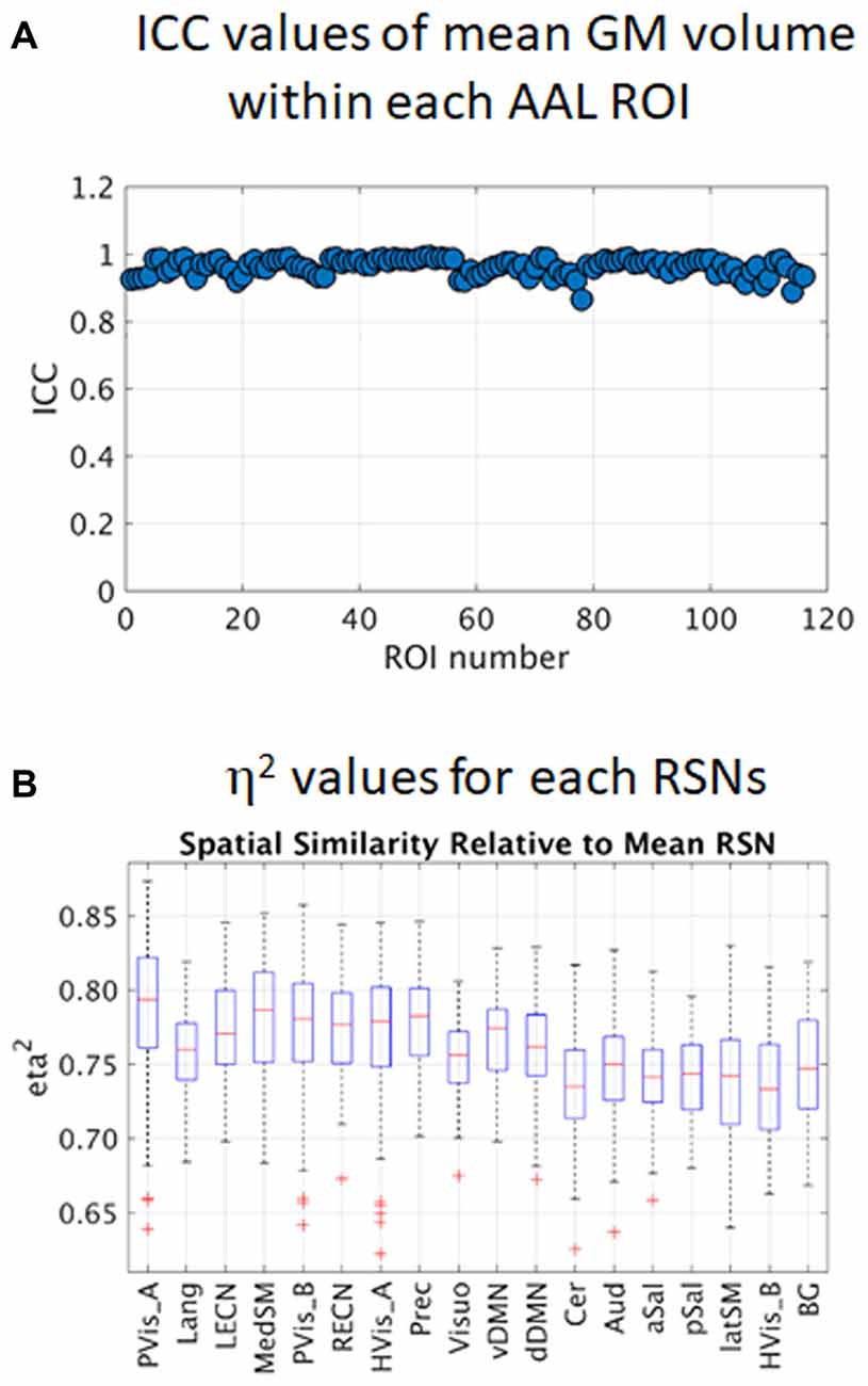
Figure 3. Intra-class correlation (ICC) values of regional gray matter (GM) volume within 116 AAL regions of interest (ROIs; A) and estimated η² values of the 18 resting state networks (RSNs; B). PVis_A, primary visual (anterior); Lang, language; LECN, left executive control; MedSM, sensorimotor (medial); PVis_B, primary visual (medial); RECN, right executive control; HVis_A, high visual (medial); Prec, precuneus; Visuo, visuospatial; vDMN, ventral default mode; dDMN, dorsal default mode; Cer, cerebellum; Aud, auditory; aSal, anterior salience; pSal, posterior salience; latSM, sensorimotor (lateral); HVis_B, high visual (lateral); BG, basal ganglia.

Low Intensity Gradient Coil Noise

Figure 1 demonstrates the effect of a faulty gradient coil on the echo planar images obtained during sessions S1 and S2. The generated gradient coil noise was not immediately visible when slices were viewed at full intensity range (Figure 1A). However, the noise, characterized by a striped pattern throughout the image, became more evident at low intensity values (Figure 1B). This gradient coil noise appeared randomly, sometimes affecting most of the volumes (and slices within the volume) in the scan, but at other times, only affecting a limited number of volumes or slices or none at all.

The performance of the proposed method for the automatic detection of volumes with gradient coil noise is illustrated in Figure 4, which shows the number of detected “noisy” volumes as a function of the threshold. From the figure, it is evident that for clean datasets, a sharp drop in the number of detected “noisy” volumes from 193 (total number of volumes) to 0 could be observed as the threshold value approached to 2. On the other hand, datasets affected with the gradient coil noise showed a different pattern. A sharp decrease in the number of detected volumes could still be observed, but the plot’s value did not completely reach 0. Instead, the plot plateaued, then slowly decreased towards 0. We surmised that the range of threshold values where the plot plateaued could serve as the effective range of intensity values separating I_bg from I_noise. The receiver operating characteristic (ROC) curves constructed from two representative noisy datasets are shown in the inset. Representative output of the automatic detection method for threshold value equal to 3 indicated by the blue vertical dash line in Figure 4 is shown in Figure 5 for two resting state fMRI data severely corrupted by the gradient coil noise. Mean background intensity for the entire image (1st row) and per slice (2nd row) showed sharp intensity increases in volumes/slices corrupted by the noise. The number of slices considered as noisy for each volume is plotted in the 3rd row with the specific noisy slices shown in the last row. A value of 3 was chosen for the threshold in the succeeding analyses since most noisy datasets have plateaued at around this value.

FIGURE 4

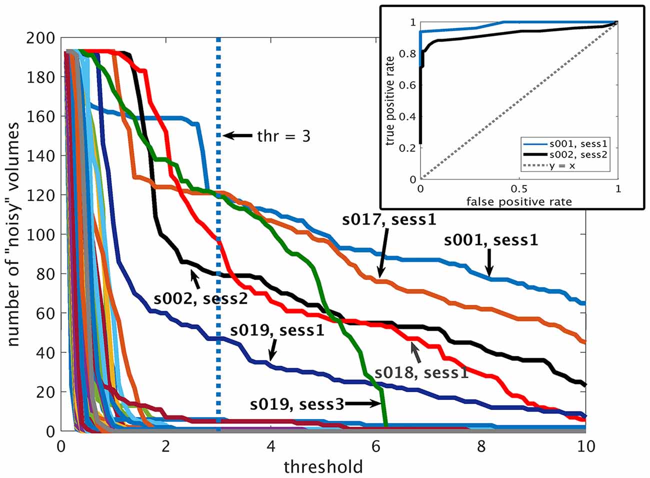
Figure 4. Performance of the proposed automatic detection method. Plots of the detected number of volumes with gradient coil noise as a function of the threshold value ranging from 0.1 to 10 for all datasets. Inset: receiver operating characteristic (ROC) curves for two representative datasets (from subject 001 in S1 and subject 002 in S2) affected by gradient coil noise.

FIGURE 5

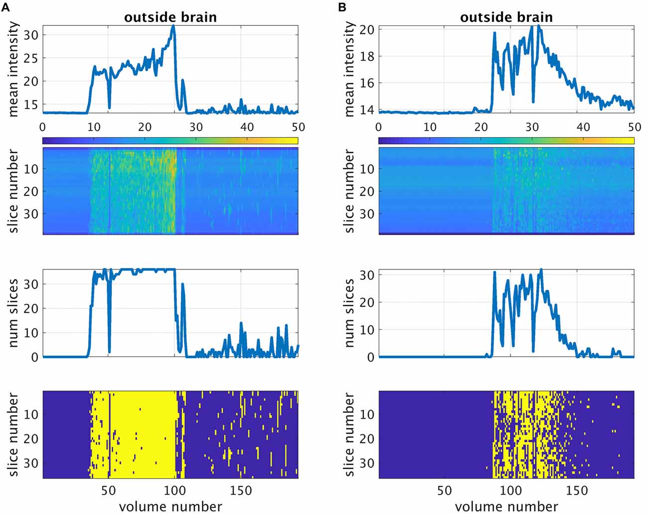
Figure 5. Detection of gradient coil noise using the approach described in the main text for two representative datasets from subject 001 (A) and subject 002 (B). The first row is the mean intensity of all voxels within the individualized outside-brain mask plotted against volume number. The second row is the mean intensity per slice. The third row is the number of slices affected by the gradient coil noise plotted against volume number as detected by the described method. The last row shows the same information per slice (shown in yellow). For this analysis, the threshold value was set to 3.

Resting state fMRI scans severely affected by gradient coil noise included those of subject 001 in S1 (Figure 5A), subject 002 in S2 (Figure 5B), subject 017 in S1, subject 018 in S1, and subject 019 in S3. We note that the last case (subject 019 in S3) was not really due to scanner noise but rather due to one of the slices that was not properly reconstructed. Some volumes from subject 019 in S1 were also affected. Censoring volumes affected by the gradient coil noise resulted in some datasets with less than 120 volumes (5 min). For this reason, we excluded some participants in the noise-corrected dual regression analyses. The number of censored volumes due to gradient coil noise is listed in Table 1. A full list of excluded participants for different comparisons is also given in Table 2.

TABLE 1

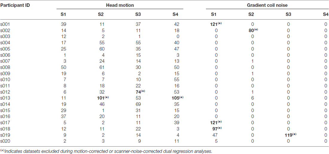
Table 1. Number of resting state functional magnetic resonance imaging (fMRI) volumes censored due to head motion (mean FD > 0.2) and gradient coil noise (threshold = 3).

TABLE 2

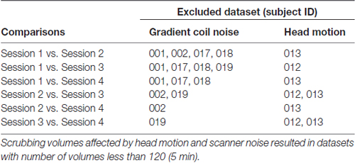
Table 2. Participants’ data excluded in paired sample comparisons for the motion-corrected and scanner-noise-corrected dual regression analyses.

Resting State Networks

From the 30 group ICs, we identified 18 components related to known RSNs. These include primary visual (anterior and posterior), high visual (medial and lateral), language, left executive, sensorimotor (medial and lateral), right executive, precuneus, visuospatial, default mode (ventral and dorsal), cerebellum, auditory, salience (anterior and posterior) and basal ganglia networks.

Mean Within Network Functional Connectivity

The mean and SD of WNFC values across participants for all sessions are summarized in Table 3. The computed ICC values for all RSNs are also included in the last column. Following the characterization of Li et al. (2015), 15 out of 18 RSNs had ICC values that could be considered as fair (>0.4). Three networks including salience (posterior and anterior) and lateral high visual networks had good ICC values (>0.6), while the language, precuneus, and ventral DMNs had poor ICC (<0.4). ICC values greater than 0.4 are still reasonable as fMRI results with ICC values ranging from 0.33 to 0.66 are considered as typically reliable (Bennett and Miller, 2010).

TABLE 3

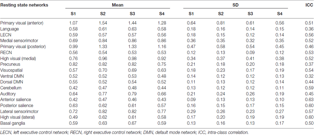
Table 3. Mean and standard deviation (SD) of within-network functional connectivity (WNFC) values across participants for each session and the estimated intra-class correlation (ICC) value.

Spatial Similarity of RSNs

Box plots of η² values for the 18 RSNs are shown in Figure 3B. The degree of spatial similarity of the participant-specific RSNs compared with the mean RSN was found to be high with mean η² values across participants and sessions ranging from 0.73 for the cerebellum (Cer) to 0.79 for the primary visual (anterior, PVis_A). Note that there were some participant-specific RSNs with η² values that were identified as outliers (red plus sign in the plot), particularly in primary visual network (PVis_A and PVis_B) and high visual network (HVis_A), with η² values below 0.7.

Dual Regression Analyses

Results of the dual regression analyses are given in Tables 4–6 and Figure 6. When no correction was performed (including all participants and volumes), clusters of voxels showing significant changes in functional connectivity between S1 and S2 could be observed in several networks including primary visual, sensorimotor, high visual, visuospatial and auditory networks (Table 4). Within-network connectivity changes for the primary visual network and high visual network are shown in Figures 6A,B (1st row). We also observed significant connectivity changes in primary visual and high visual networks between S1 and S3, and in high visual network between S1 and S4. On the other hand, the cerebellum showed significant connectivity changes between S3 and S4.

TABLE 4

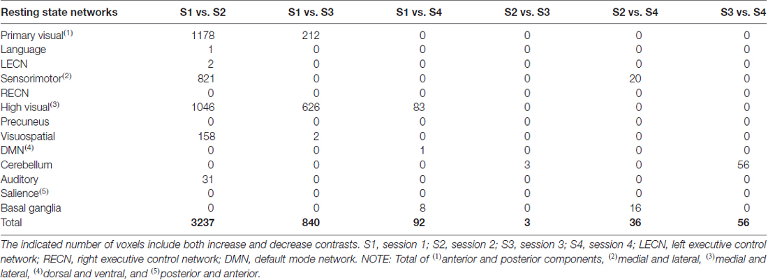
Table 4. Voxel count for no-correction dual regression analyses.

TABLE 5

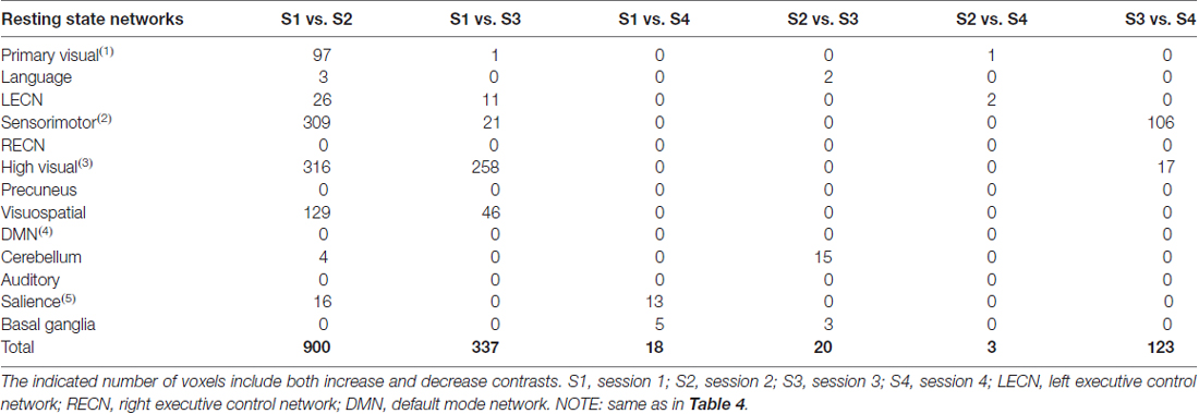
Table 5. Voxel count for motion-corrected dual regression analyses.

TABLE 6

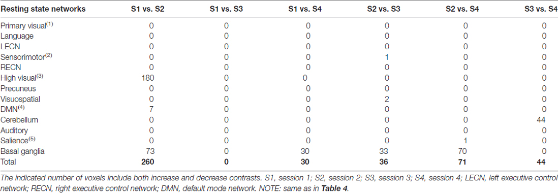
Table 6. Voxel count for gradient-coil-noise-corrected dual regression analyses.

FIGURE 6

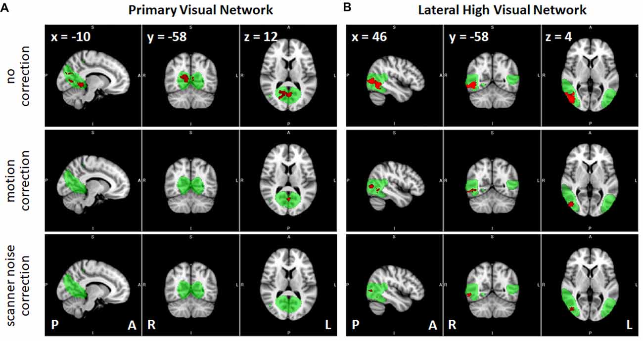
Figure 6. Effects of the correction methods in removing the spurious significant connectivity changes, shown in red, between sessions S1 and S2 observed in (A) primary visual network and (B) high visual network (lateral). RSNs are shown in green (group independent components (ICs) z > 3). P, posterior; A, anterior; L, left; R, right.

Correcting for the effect of head motion by censoring volumes with FD values greater than 0.2 reduced the number of voxels exhibiting significant connectivity changes between S1 and S2 (Table 5). In particular, the number of voxels in the primary visual, sensorimotor and high visual networks was significantly reduced when head motion was taken into account. This is also evident in Figure 6 (2nd row). On the other hand, the effect of head motion correction on the connectivity changes in the visuospatial networks was relatively modest. Between S1 and S3, significant changes in connectivity in the (primary/high) visual networks was also reduced, although some other networks (LECN, sensorimotor and visuospatial) also exhibited a slight increase in the number of voxels showing significant connectivity changes. The observed changes in the cerebellum for the no-correction analysis between S3 and S4 disappeared, indicating that the observed change could be driven by motion artifact. The sensorimotor network, however, showed an increase in the number of voxels, which was not observed in the no-correction analysis. Overall, we could observe a reduction in the number of voxel showing significant connectivity changes when head motion was taken into account. The list of the number of censored volumes for each participant and session is given in Table 1 and the list of participants excluded in the motion-corrected analyses due to excessive head motion is given in Table 2.

When datasets were corrected for gradient coil noise, the number of voxels exhibiting connectivity changes was significantly reduced especially in comparisons involving S1 (Table 6). Specifically, the total number of significant voxels was reduced from 3237, 840 and 92 in no-correction analyses to 260, 0 and 30 in noise-corrected analyses in S1 vs. S2, S1 vs. S3 and S1 vs. S4, respectively. Figures 6A,B (3rd row) shows the case for the visual networks. This clearly suggests that the observed connectivity changes were spurious and mainly due to the gradient coil noise in resting state fMRI data acquired before the gradient coil was replaced. The remaining voxels with significant connectivity changes could be due to other factors including motion artifact. For instance, the number of voxels in high visual network was reduced when motion was taken into account. Thus, the remaining 180 voxels in this network could just be due to head motion. In addition, the 44 voxels observed in the cerebellum in S3 vs. S4 comparison could also be due to motion as this cluster disappeared when the analysis was corrected for motion. Compared to the no-correction analyses, we also observed an increase in the number of voxels showing significant connectivity changes in the basal ganglia network especially in comparisons involving S2. Again, this could be driven by head motion as the number of voxels with significant connectivity changes in this network were very limited in the motion-corrected analyses (Table 5) and subject 013 had high motion data in both S2 and S4 (Table 1). Based on these results, censoring volumes affected by gradient coil noise could lead to reproducible RSNs on datasets obtained with the same gradient coil (i.e., S1 vs. S2 and S3 vs. S4) and between different gradient coils (i.e., S1 vs. S3, S1 vs. S4, S2 vs. S3 and S2 vs. S4).

Unfortunately, simultaneously censoring both gradient coil noise and head motion was not possible since it would result to several datasets with volumes less than 120. However for completeness, we included in Supplementary Table S1 (excluded data sets) and Supplementary Table S2 (voxel count) the case where both gradient coil noise and head motion were simultaneously censored lowering the minimum number of volumes to 96 (4 min) and for a limited data set.

Discussion

We examined the effect of low intensity gradient coil noise and gradient coil replacement on the reproducibility of T1-weighted images and resting state fMRI data. Our main findings showed that: (1) T1-weighted images were not affected by this noise and metrics derived from T1 were highly reproducible even after gradient coil replacement; (2) in spite of being low in intensity, the observed gradient-coil-generated noise could introduce significant connectivity changes in several RSNs affecting WNFC values, which consequently, resulted to only fair ICC values; and (3) these spurious connectivity changes could be eliminated by censoring volumes corrupted by gradient coil noise in the same manner as minimizing the effects of head motion by censoring volumes with high motion (Power et al., 2015). After gradient coil noise correction, spurious connectivity changes were significantly reduced, if not completely removed, in comparisons between sessions within the same gradient coil (S1 vs. S2) and across different gradient coils (e.g., S1 vs. S3 and S2 vs. S4) suggesting the reproducibility of RSNs before and after gradient coil replacement.

RSN Reproducibility

Previous studies have shown that RSNs are reproducible within participants over durations of weeks to months (Damoiseaux et al., 2006; Wisner et al., 2013) and even longer periods (Guo et al., 2012; Choe et al., 2015). A study comparing test-retest reliability of resting state fMRI data using temporal signal to noise ratio (tSNR) within two RSNs as a metric after a major hardware repair had also shown consistent tSNR across conditions (Huang et al., 2012). However, the authors did not mention the presence of noise in the used resting state fMRI data before gradient coil replacement or considered the effect of noise on the reproducibility of resting state fMRI.

In this study, we have focused on the effect of gradient coil noise on the reproducibility of RSNs. Our results showed that before the gradient coil was changed, the gradient coil noise significantly affected several RSNs in terms of spurious detectable connectivity changes. The gradient coil noise also affected the estimates of the mean WNFC as can be seen in Table 3, where the primary visual (anterior) and high visual (medial) networks have relatively lower WNFC values in S1, where most of the gradient coil noise was observed, compared to other sessions. This, in turn, could have affected the estimates of the ICC values resulting in a relatively fair reliability of the networks. The box plots of the spatial similarity measure η² (Figure 3B) showed several outliers which could again be driven by the presence of the gradient coil noise in some resting state fMRI data before the gradient coil was replaced.

To mitigate this issue, we introduced a technique which significantly reduced, if not completely removed, spurious connectivity changes driven by the gradient coil noise in some resting state fMRI data. We employed a similar method, called scrubbing or censoring, used to minimize motion artifacts in the presence of large head motion (Power et al., 2015). Application of this method reduced the number of voxels exhibiting spurious connectivity changes in all networks, except in high visual and basal ganglia networks, in comparisons involving S1. The remaining voxels could be just due to other factors including motion artifact. The disadvantage of the method is that it reduced the number of volumes included in the analysis and led to the exclusion of the entire dataset for extremely noisy scans. In this case, a method that would only remove the noise from the image without discarding the volumes in the analysis would be more beneficial.

Another concern with censoring relates to the differences in the number of volumes included in the analysis (degrees of freedom) for each participant, which could introduce variability in the estimates of the correlation values. In our analysis, we set the minimum number of volumes to 120 (5 min) and datasets with volumes less than this minimum were excluded. As shown by Van Dijk et al. (2010), estimates of correlation strengths started to stabilize with acquisition times as brief as 5 min. We can therefore assume that in the preceding analyses the variability introduced due to the differences in the number of volumes would be minimal. Moreover, for the noise-corrected analyses, most of the datasets with censored volumes were excluded and only one dataset (subject 019 in S1) where the number of censored volumes was greater than six was included. The findings of these analyses were therefore minimally affected by this issue. For the motion-corrected analyses, the number of censored volumes for each participant did vary from session to session. Thus, the results of these analyses should be carefully interpreted with this potential limitation.

T1 Anatomical Image

With ICC values close to 1, our ROI-based analysis of GM images revealed high reproducibility across gradient coil replacement. This is further confirmed using a direct voxel-wise comparison between sessions showing no significant changes observed in statistical maps using a statistical threshold of p < 0.05 FWE-corrected for multiple comparisons, a standard practice for voxel-based morphometric analysis. This is consistent with the observation that the faulty gradient coil had not yet affected T1-weighted images and had not introduced any artifact into these images. This finding is also consistent with that of Huang et al. (2012) showing high reproducibility of the volumes of selected ROIs as stability metrics for T1 images after gradient coil replacement.

Detection of Gradient Noise

We also proposed a reliable method to automatically detect the gradient coil noise from the resting state fMRI data. The method relied on the noise characteristics observed in our dataset. In particular, it assumed that the mean intensity of the background image (outside brain) was constant in the absence of gradient coil noise. Under this condition, the method worked quite satisfactorily. It may also work with other types of randomly occurring image artifacts such as image reconstruction failures as demonstrated in one of the resting state fMRI data. However, its general applicability to other types of noise will depend on the characteristics of the noise being considered.

Another important issue to consider for the method’s general applicability is the proper choice of the threshold value to use in detecting noisy slices or volumes. Here, we used a threshold value of 3, which appeared to be optimal for the current datasets. However, this may not be the case for other datasets. Choosing the appropriate threshold value is important especially when using censoring to minimize spurious findings. Interestingly, the plots showing the number of detected “noisy” volumes as a function of the threshold (Figure 4) could provide some useful hints in selecting the appropriate threshold value. As we have mentioned in the results section, the observed plateau in the plot could indicate the range of threshold values separating I_bg from I_noise. Given this, the value where the plot starts to plateau could therefore be used as the appropriate threshold. This worked for most of our noisy datasets, although its general applicability still remains to be validated.

Conclusion

In summary, hardware-related noise such as those due to a faulty gradient coil could significantly affect the reproducibility of RSNs. In spite of its low intensity, this type of noise could introduce spurious connectivity changes in several RSNs, which could be easily mistaken as valid changes. By censoring corrupted image volumes during the analysis, the number of spurious connectivity could be significantly minimized if not completely removed. Applying this correction method could also make RSNs reproducible even after gradient coil replacement. These findings suggest that, with an appropriate correction method, resting state fMRI datasets affected by hardware problems could still be used to generate consistent and reproducible RSNs.

Author Contributions

EB, SK, HI, HW, SM, SN and GS conceived and designed the study. EB, ET, YY, YO, MK, TO, SK and HI performed the experiments and analyzed the dataset. EB, HI, HW and SM wrote the draft of the manuscript and all authors reviewed and approved the final manuscript.

Funding

This work was supported by Grants-in-Aid from the Research Committee of Central Nervous System Degenerative Diseases by the Ministry of Health, Labour and Welfare and from the Integrated Research on Neuropsychiatric Disorders project carried out under the Strategic Research for Brain Sciences by the Ministry of Education, Culture, Sports, Science and Technology of Japan. This work was also supported by a Grant-in-Aid for Scientific Research from the Ministry of Education, Culture, Sports, Science and Technology (MEXT) of Japan (grant number 80569781), and a Grant-in-Aid for Scientific Research on Innovative Areas (Brain Protein Aging and Dementia Control; 26117002) from MEXT.

Conflict of Interest Statement

The authors declare that the research was conducted in the absence of any commercial or financial relationships that could be construed as a potential conflict of interest.

Footnotes

1. ^ http://fsl.fmrib.ox.ac.uk/fsl/fslwiki/
2. ^ http://findlab.stanford.edu/functional_ROIs.html

Supplementary Material

The Supplementary Material for this article can be found online at: https://www.frontiersin.org/articles/10.3389/fnhum.2018.00148/full#supplementary-material

References

Ashburner, J. (2007). A fast diffeomorphic image registration algorithm. Neuroimage 38, 95–113. doi: 10.1016/j.neuroimage.2007.07.007

PubMed Abstract | CrossRef Full Text | Google Scholar

Ashburner, J., and Friston, K. J. (2000). Voxel-based morphometry—The methods. Neuroimage 11, 805–821. doi: 10.1006/nimg.2000.0582

PubMed Abstract | CrossRef Full Text | Google Scholar

Baliki, M. N., Geha, P. Y., Apkarian, A. V., and Chialvo, D. R. (2008). Beyond feeling: chronic pain hurts the brain, disrupting the default-mode network dynamics. J. Neurosci. 28, 1398–1403. doi: 10.1523/JNEUROSCI.4123-07.2008

PubMed Abstract | CrossRef Full Text | Google Scholar

Baliki, M. N., Mansour, A. R., Baria, A. T., and Apkarian, A. V. (2014). Functional reorganization of the default mode network across chronic pain conditions. PLoS One 9:e106133. doi: 10.1371/journal.pone.0106133

PubMed Abstract | CrossRef Full Text | Google Scholar

Beckmann, C. F., DeLuca, M., Devlin, J. T., and Smith, S. M. (2005). Investigations into resting-state connectivity using independent component analysis. Philos. Trans. R. Soc. Lond. B Biol. Sci. 360, 1001–1013. doi: 10.1098/rstb.2005.1634

PubMed Abstract | CrossRef Full Text | Google Scholar

Bennett, C. M., and Miller, M. B. (2010). How reliable are the results from functional magnetic resonance imaging? Ann. N Y Acad. Sci. 1191, 133–155. doi: 10.1111/j.1749-6632.2010.05446.x

PubMed Abstract | CrossRef Full Text | Google Scholar

Betzel, R. F., Byrge, L., He, Y., Goñi, J., Zuo, X. N., and Sporns, O. (2014). Changes in structural and functional connectivity among resting-state networks across the human lifespan. Neuroimage 102, 345–357. doi: 10.1016/j.neuroimage.2014.07.067

PubMed Abstract | CrossRef Full Text | Google Scholar

Chen, S., Ross, T. J., Zhan, W., Myers, C. S., Chuang, K. S., Heishman, S. J., et al. (2008). Group independent component analysis reveals consistent resting-state networks across multiple sessions. Brain Res. 1239, 141–151. doi: 10.1016/j.brainres.2008.08.028

PubMed Abstract | CrossRef Full Text | Google Scholar

Choe, A. S., Jones, C. K., Joel, S. E., Muschelli, J., Belegu, V., Caffo, B. S., et al. (2015). Reproducibility and temporal structure in weekly resting-state fMRI over a period of 3.5 years. PLoS One 10:e0140134. doi: 10.1371/journal.pone.0140134

PubMed Abstract | CrossRef Full Text | Google Scholar

Cohen, A. L., Fair, D. A., Dosenbach, N. U. F., Miezin, F. M., Dierker, D., Van Essen, D. C., et al. (2008). Defining functional areas in individual human brains using resting functional connectivity MRI. Neuroimage 41, 45–57. doi: 10.1016/j.neuroimage.2008.01.066

PubMed Abstract | CrossRef Full Text | Google Scholar

Dai, Z., Yan, C., Li, K., Wang, Z., Wang, J., Cao, M., et al. (2015). Identifying and mapping connectivity patterns of brain network hubs in Alzheimer’s disease. Cereb. Cortex 25, 3723–3742. doi: 10.1093/cercor/bhu246

PubMed Abstract | CrossRef Full Text | Google Scholar

Damoiseaux, J. S., Rombouts, S. A. R. B., Barkhof, F., Scheltens, P., Stam, C. J., Smith, S. M., et al. (2006). Consistent resting-state networks across healthy subjects. Proc. Natl. Acad. Sci. U S A 103, 13848–13853. doi: 10.1073/pnas.0601417103

PubMed Abstract | CrossRef Full Text | Google Scholar

Esposito, R., Mattei, P. A., Briganti, C., Romani, G. L., Tartaro, A., and Caulo, M. (2012). Modifications of default-mode network connectivity in patients with cerebral glioma. PLoS One 7:e40231. doi: 10.1371/journal.pone.0040231

PubMed Abstract | CrossRef Full Text | Google Scholar

Filippini, N., MacIntosh, B. J., Hough, M. G., Goodwin, G. M., Frisoni, G. B., Smith, S. M., et al. (2009). Distinct patterns of brain activity in young carriers of the APOE-ε4 allele. Proc. Natl. Acad. Sci. U S A 106, 7209–7214. doi: 10.1073/pnas.0811879106

PubMed Abstract | CrossRef Full Text | Google Scholar

Fox, M. D., and Greicius, M. (2010). Clinical applications of resting state functional connectivity. Front. Syst. Neurosci. 4:19. doi: 10.3389/fnsys.2010.00019

PubMed Abstract | CrossRef Full Text | Google Scholar

Fox, M. D., Snyder, A. Z., Vincent, J. L., Corbetta, M., Van Essen, D. C., and Raichle, M. E. (2005). The human brain is intrinsically organized into dynamic, anticorrelated functional networks. Proc. Natl. Acad. Sci. U S A 102, 9673–9678. doi: 10.1073/pnas.0504136102

PubMed Abstract | CrossRef Full Text | Google Scholar

Fransson, P., Skiöld, B., Horsch, S., Nordell, A., Blennow, M., Lagercrantz, H., et al. (2007). Resting-state networks in the infant brain. Proc. Natl. Acad. Sci. U S A 104, 15531–15536. doi: 10.1073/pnas.0704380104

PubMed Abstract | CrossRef Full Text | Google Scholar

Greicius, M. (2008). Resting-state functional connectivity in neuropsychiatric disorders. Curr. Opin. Neurol. 21, 424–430. doi: 10.1097/wco.0b013e328306f2c5

PubMed Abstract | CrossRef Full Text | Google Scholar

Greicius, M. D., Krasnow, B., Reiss, A. L., and Menon, V. (2003). Functional connectivity in the resting brain: a network analysis of the default mode hypothesis. Proc. Natl. Acad. Sci. U S A 100, 253–258. doi: 10.1073/pnas.0135058100

PubMed Abstract | CrossRef Full Text | Google Scholar

Greicius, M. D., Srivastava, G., Reiss, A. L., and Menon, V. (2004). Default-mode network activity distinguishes Alzheimer’s disease from healthy aging: evidence from functional MRI. Proc. Natl. Acad. Sci. U S A 101, 4637–4642. doi: 10.1073/pnas.0308627101

PubMed Abstract | CrossRef Full Text | Google Scholar

Guo, C. C., Kurth, F., Zhou, J., Mayer, E. A., Eickhoff, S. B., Kramer, J. H., et al. (2012). One-year test-retest reliability of intrinsic connectivity network fMRI in older adults. Neuroimage 61, 1471–1483. doi: 10.1016/j.neuroimage.2012.03.027

PubMed Abstract | CrossRef Full Text | Google Scholar

Hacker, C. D., Perlmutter, J. S., Criswell, S. R., Ances, B. M., and Snyder, A. Z. (2012). Resting state functional connectivity of the striatum in Parkinson’s disease. Brain 135, 3699–3711. doi: 10.1093/brain/aws281

PubMed Abstract | CrossRef Full Text | Google Scholar

Huang, L., Wang, X., Baliki, M. N., Wang, L., Apkarian, A. V., and Parrish, T. B. (2012). Reproducibility of structural, resting-state BOLD and DTI data between identical scanners. PLoS One 7:e47684. doi: 10.1371/journal.pone.0047684

PubMed Abstract | CrossRef Full Text | Google Scholar

Lee, M. H., Smyser, C. D., and Shimony, J. S. (2013). Resting-state fMRI: a review of methods and clinical applications. AJNR Am. J. Neuroradiol. 34, 1866–1872. doi: 10.3174/ajnr.a3263

PubMed Abstract | CrossRef Full Text | Google Scholar

Li, Z., Liu, M., Lan, L., Zeng, F., Makris, N., Liang, Y., et al. (2016). Altered periaqueductal gray resting state functional connectivity in migraine and the modulation effect of treatment. Sci. Rep. 6:20298. doi: 10.1038/srep20298

PubMed Abstract | CrossRef Full Text | Google Scholar

Li, L., Zeng, L., Lin, Z. J., Cazzell, M., and Liu, H. (2015). Tutorial on use of intraclass correlation coefficients for assessing intertest reliability and its application in functional near-infrared spectroscopy-based brain imaging. J. Biomed. Opt. 20:50801. doi: 10.1117/1.jbo.20.5.050801

PubMed Abstract | CrossRef Full Text | Google Scholar

Maesawa, S., Bagarinao, E., Fujii, M., Futamura, M., Motomura, K., Watanabe, H., et al. (2015). Evaluation of resting state networks in patients with gliomas: connectivity changes in the unaffected side and its relation to cognitive function. PLoS One 10:e0118072. doi: 10.1371/journal.pone.0118072

PubMed Abstract | CrossRef Full Text | Google Scholar

Martucci, K. T., Shirer, W. R., Bagarinao, E., Johnson, K. A., Farmer, M. A., Labus, J. S., et al. (2015). The posterior medial cortex in urologic chronic pelvic pain syndrome: detachment from default mode network-a resting-state study from the MAPP Research Network. Pain 156, 1755–1764. doi: 10.1097/j.pain.0000000000000238

PubMed Abstract | CrossRef Full Text | Google Scholar

Mugler, J. P. III., and Brookeman, J. R. (1990). Three-dimensional magnetization-prepared rapid gradient-echo imaging (3D MP RAGE). Magn. Reson. Med. 15, 152–157. doi: 10.1002/mrm.1910150117

PubMed Abstract | CrossRef Full Text | Google Scholar

Nichols, T. E., and Holmes, A. P. (2002). Nonparametric permutation tests for functional neuroimaging: a primer with examples. Hum. Brain Mapp. 15, 1–25. doi: 10.1002/hbm.1058

PubMed Abstract | CrossRef Full Text | Google Scholar

Power, J. D., Barnes, K. A., Snyder, A. Z., Schlaggar, B. L., and Petersen, S. E. (2012). Spurious but systematic correlations in functional connectivity MRI networks arise from subject motion. Neuroimage 59, 2142–2154. doi: 10.1016/j.neuroimage.2011.10.018

PubMed Abstract | CrossRef Full Text | Google Scholar

Power, J. D., Mitra, A., Laumann, T. O., Snyder, A. Z., Schlaggar, B. L., and Petersen, S. E. (2014). Methods to detect, characterize and remove motion artifact in resting state fMRI. Neuroimage 84, 320–341. doi: 10.1016/j.neuroimage.2013.08.048

PubMed Abstract | CrossRef Full Text | Google Scholar

Power, J. D., Schlaggar, B. L., and Petersen, S. E. (2015). Recent progress and outstanding issues in motion correction in resting state fMRI. Neuroimage 105, 536–551. doi: 10.1016/j.neuroimage.2014.10.044

PubMed Abstract | CrossRef Full Text | Google Scholar

Sala-Llonch, R., Bartrés-Faz, D., and Junqué, C. (2015). Reorganization of brain networks in aging: a review of functional connectivity studies. Front. Psychol. 6:663. doi: 10.3389/fpsyg.2015.00663

PubMed Abstract | CrossRef Full Text | Google Scholar

Shimony, J. S., Zhang, D., Johnston, J. M., Fox, M. D., Roy, A., and Leuthardt, E. C. (2009). Resting-state spontaneous fluctuations in brain activity. Acad. Radiol. 16, 578–583. doi: 10.1016/j.acra.2009.02.001

PubMed Abstract | CrossRef Full Text | Google Scholar

Shirer, W. R., Ryali, S., Rykhlevskaia, E., Menon, V., and Greicius, M. D. (2012). Decoding subject-driven cognitive states with whole-brain connectivity patterns. Cereb. Cortex 22, 158–165. doi: 10.1093/cercor/bhr099

PubMed Abstract | CrossRef Full Text | Google Scholar

Shrout, P. E., and Fleiss, J. L. (1979). Intraclass correlations: uses in assessing rater reliability. Psychol. Bull. 86, 420–428. doi: 10.1037/0033-2909.86.2.420

PubMed Abstract | CrossRef Full Text | Google Scholar

Smith, S. M., and Nichols, T. E. (2009). Threshold-free cluster enhancement: addressing problems of smoothing, threshold dependence and localisation in cluster inference. Neuroimage 44, 83–98. doi: 10.1016/j.neuroimage.2008.03.061

PubMed Abstract | CrossRef Full Text | Google Scholar

Smyser, C. D., Inder, T. E., Shimony, J. S., Hill, J. E., Degnan, A. J., Snyder, A. Z., et al. (2010). Longitudinal analysis of neural network development in preterm infants. Cereb. Cortex 20, 2852–2862. doi: 10.1093/cercor/bhq035

PubMed Abstract | CrossRef Full Text | Google Scholar

Szewczyk-Krolikowski, K., Menke, R. A. L., Rolinski, M., Duff, E., Salimi-Khorshidi, G., Filippini, N., et al. (2014). Functional connectivity in the basal ganglia network differentiates PD patients from controls. Neurology 83, 208–214. doi: 10.1212/WNL.0000000000000592

PubMed Abstract | CrossRef Full Text | Google Scholar

Tomasi, D., and Volkow, N. D. (2012). Aging and functional brain networks. Mol. Psychiatry 17, 549–558. doi: 10.1038/mp.2011.81

CrossRef Full Text | Google Scholar

Tzourio-Mazoyer, N., Landeau, B., Papathanassiou, D., Crivello, F., Etard, O., Delcroix, N., et al. (2002). Automated anatomical labeling of activations in SPM using a macroscopic anatomical parcellation of the MNI MRI single-subject brain. Neuroimage 15, 273–289. doi: 10.1006/nimg.2001.0978

PubMed Abstract | CrossRef Full Text | Google Scholar

Van Dijk, K. R. A., Hedden, T., Venkataraman, A., Evans, K. C., Lazar, S. W., and Buckner, R. L. (2010). Intrinsic functional connectivity as a tool for human connectomics: theory, properties and optimization. J. Neurophysiol. 103, 297–321. doi: 10.1152/jn.00783.2009

PubMed Abstract | CrossRef Full Text | Google Scholar

Wisner, K. M., Atluri, G., Lim, K. O., and MacDonald, A. W. III. (2013). Neurometrics of intrinsic connectivity networks at rest using fMRI: retest reliability and cross-validation using a meta-level method. Neuroimage 76, 236–251. doi: 10.1016/j.neuroimage.2013.02.066

PubMed Abstract | CrossRef Full Text | Google Scholar

Yao, N., Chang Shek-Kwan, R., Cheung, C., Pang, S., Lau, K. K., Suckling, J., et al. (2014). The default mode network is disrupted in Parkinson’s disease with visual hallucinations. Hum. Brain Mapp. 35, 5658–5666. doi: 10.1002/hbm.22577

PubMed Abstract | CrossRef Full Text | Google Scholar

Zuo, X. N., Kelly, C., Adelstein, J. S., Klein, D. F., Castellanos, F. X., and Milham, M. P. (2010). Reliable intrinsic connectivity networks: test-retest evaluation using ICA and dual regression approach. Neuroimage 49, 2163–2177. doi: 10.1016/j.neuroimage.2009.10.080

PubMed Abstract | CrossRef Full Text | Google Scholar