Cross-validated tree-based models for multi-target learning

1 Introduction

Multi-target learning (MTL) is a supervised learning paradigm that aims to construct a predictive model to multiple response variables from a common set of features. This paradigm is also known as multi-variate (Brown and Zidek, 1980; Breiman and Friedman, 1997) or multi-output learning (Liu et al., 2009; Yao et al., 2020), and has been an active research area for over four decades (Izenman, 1975). MTL applies to a wide range of fields due to its fundamental nature. For example, Ghosn and Bengio (1996) used artificial neural networks (ANNs) to predict stocks investment profits over time. They considered 3,636 assets from Canadian large-capitalization stocks and from the Canadian treasury. A series of experiments showed a major improvement by allowing different levels of shared parameters among the targets. Other notable examples include chemometrics (Burnham et al., 1999), ecological modeling (Kocev et al., 2009), text classification (Schapire and Singer, 2000), and bioinformatics (Ji et al., 2008).

There are two main approaches for MTL. The first is typically referred to as problem transformation methods or local methods. It transforms the MTL problem into a series of single-target models, and single-output schemes are applied. The second approach is mostly known as algorithm adaptation or global methods. These methods train a single model simultaneously for all the targets. None of these approaches can universally outperform the other. Indeed, both have certain merits and limitations, as demonstrated in the following sections. The interested reader is referred to Adıyeke and Baydoğan (2020) for a thorough discussion.

Decision trees are among the most popular supervised learning schemes (Wu et al., 2008). Decision trees hold many favorable properties. They are simple to understand and interpret, able to handle numerical and categorical features and have the ability to capture non-linear and non-additive relationships. Training a decision tree typically requires recursive partitioning of the feature space into a set of rectangles. Several popular decision tree implementations were proposed over the years. For example, ID3 (Quinlan, 1986), CART (Li et al., 1984), C4.5/C5.0 (Quinlan, 2004, 2014) to name a few.

MTL has been utilizes to a variety of predictive models. In the context of decision-tree methods, there are two major MTL approaches. The first is to construct a single tree for each response variable (Kocev et al., 2009). The second is to train a joint tree for all response variables all together (De'Ath, 2002). A hybrid approach, which combines the two, is also considered in the literature (Santos et al., 2021; Alves and Cerri, 2022). In this work we introduce a new hybrid tree-based MTL framework. Specifically, we train decision trees that share some levels for all the targets, while allowing other levels to be target specific. Our proposed framework is motivated by the observation that both single and joint trees hold unique advantages in different scenarios. Single trees are advantageous in cases where the correlation between response variables are weak or non-existent, as they allow the flexibility to train more tailored models for each response variable. On the other hand, training a joint tree for all response variables can account for the relationship between the targets, if such exists. In this work we propose a hybrid approach that selects the appropriate method at each node by utilizing a cross-validation (CV) score. Specifically, the proposed approach determines whether to create a separate tree for each response variable or to build a joint tree for all response variables at each node based on its CV score. By combining the advantages of both schemes, our method adapts to the unique properties of the problem, resulting in improved predictive performance. Overall, our proposed hybrid approach offers a more flexible and effective solution compared to traditional methods. Our experiments demonstrate favorable performance compared to existing methods on various synthetic and real-world datasets. An implementation of the proposed method is publicly available.¹

2 Related work

In this section we first overview existing multi-target algorithms. Next, we present the CART algorithm and describe the building process of the tree. Then, we introduce the ALOOF method, a novel approach to variable selection, which we adapt in our proposed framework. Finally, we discuss currently known multi-target tree-based algorithms.

2.1 Multi target learning

The MTL framework considers n independent observations from p features and d targets. Specifically, we denote the i^th observation as (x_i, y_i) where x_i = (x_i1, x_i2…x_ip) and y_i = (y_i1, y_i2…y_id). Notice that all d targets share the same set of features. As mentioned above, current MTL methods are typically either local or global, where each approach holds its own advantages and caveats.

2.1.1 Local MTL methods

2.1.1.1 The single target scheme

The most basic local approach is the baseline single target (ST) scheme (Spyromitros-Xioufis et al., 2016). Here, d separate models are learned for each target independently. Specifically, for response variable r, ST considers a training set $T_r={\left\{x_i,y_{ir}\right\}}_{i=1}^n$ where x_i is the original feature vector x_i = (x_i1, x_i2…x_ip).

2.1.1.2 Stacked single target

Stacked Single Target (SST) (Spyromitros-Xioufis et al., 2016) is an MTL scheme for regression tasks, inspired by the multi-label classification method Stacked Binary Relevance (SBR) (Godbole and Sarawagi, 2004). The SST training process consists of two stages. First, d single models are separately trained for each response variable, as in ST. Then, d meta-models, one for each response variable, are trained in the second stage. Each meta-model is trained on a transformed training set $T_r^{\prime }={\left\{x_i^{\prime },y_{ir}\right\}}_{i=1}^n$, where $x_i^{\prime }=(x_{i1},\dots ,x_{ip},{ŷ}_{i1},\dots ,{ŷ}_{id})$ is the original feature vector x_i, augmented with the predictions from the first stage.

2.1.1.3 Regressor and classifier chains

Regressor Chains (RC) (Spyromitros-Xioufis et al., 2016) and Classifier Chains (CC) (Read et al., 2011) train d models, similar in spirit to SST. Here, we first set a (random) order among the targets. Then, each target is trained on the predictions of the previous targets in the drawn order. For example, assume that d = 2 and the drawn order of targets is (y₂, y₁). Then, the training set for the first response variable y₂ is $T_2^{\prime }={\left\{x_i^{\prime },y_{i2}\right\}}_{i=1}^n$, where $x_i^{\prime }$ is the original features vector. Next, we proceed to y₁. The transformed training set for this target is $T_1^{\prime }={\left\{x_i^{\prime },y_{i1}\right\}}_{i=1}^n$ where now $x_i^{\prime }=(x_{i1},\dots ,x_{ip},{ŷ}_{i2})$ is the original feature vector, augmented with the ŷ_i2 from the previous step.

2.1.2 Global MTL methods

Michelucci and Venturini (2019) proposed an MTL neural network architecture, consisting of common (joint) and individual hidden layers (see Figure 1). The common hidden layers consider all response variables simultaneously, as they strive to capture the dependencies among them. The outputs of these layers are used as inputs for the following individual layers. These, on the other hand, focus on the unique properties of each separate response and allow introduce flexibility to their proposed scheme.

Figure 1

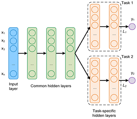
Figure 1. An example of a MTL network architecture with two targets (tasks).

Evgeniou and Pontil (2004) presented a different MTL method using a regularization approach. They focused on support vector machines (SVM) and extended this notion to the MTL setup. In SVM, the objective is to find a hyper-plane w^Tx − b = 0 with the largest distance to the nearest training data points of each class. Under the assumption that all targets' weight vectors w are “close to each other”, they defined the weight of the r^th target w_r as w_r = w₀ + v_r where w₀ is the mean of the w's over all targets and v_r corresponds to the deviation from the mean. The objective function is similar to the single target scheme, with a summation of the parameters across all the targets. It contains two positive regularization parameters, for the two terms. The regularization parameters impose constraints and control the variability among the models.

Curds and Whey (C&W) is a procedure proposed by Breiman and Friedman (1997), for multiple linear regression with multivariate responses. C&W utilizes elements of canonical correlation and shrinkage estimation to enhance the prediction accuracy for each response variable. Specifically, C&W applies simple least squares regressions and then utilizes the correlations between the responses and features to shrink the predicted values from those regressions.

2.2 Classification and regression trees

As mentioned above, the focus of our work is the design of a decision tree-based MTL framework. For this purpose, we briefly review the popular Classification and Regression Tree (CART) algorithm. Consider n observations ${\left\{x_i,y_i\right\}}_{i=1}^n$ consisting of p features, where x_i = (x_i1, x_i2…x_ip) and y_i is a real (regression) or categorical (classification) scalar. During the training phase of the tree, CART performs recursive binary partitioning of the feature space. For each feature j we consider a collection of possible split points S_j. Every split point s ∈ S_j corresponds to a binary partition of the n observation into two disjoint sets L(s) and R(s). For numerical/ordinal features the two sets define (without loss of generality) L(s) = {X|X_j < s} and R(s) = {X|X_j ≥ s}. Notice that in this case, |S_j| < n as only unique values are considered along the sorted values. For categorical features the two sets are define as L(s) = {X|X_j ∈ Q_jL} and R(s) = {X|X_j ∈ Q_jR} where Q_j is the set of categories of variable j and Q_jL, Q_jR are sub-sets such that Q_jL ∪ Q_jR = Q_j and Q_jL ∩ Q_jR = ∅. Here, there is a total of $\left|S_j\right|=2^{\left|Q_j\right|-1}-1$ possible binary splits. However, it is easy to show that one can order the categories by the corresponding mean of their response variables, and only consider the splits along this ordered list (Li et al., 1984). This leads to a total of |Q_j|−1 candidate splits. For every split s ∈ S_j, CART evaluates a loss criterion. In regression trees the popular choice is the squared loss,

$\begin{array}{ll}\mathcal{L}(s)={\Sigma }_{i\in L(s)}{(y_i-{ȳ}_L)}^2+{\Sigma }_{i\in R(s)}{(y_i-{ȳ}_R)}^2& (1)\end{array}$

where ȳ_L and ȳ_R are the mean over the sets L(s) and R(s), respectively. For a two-class classification tree it utilizes the Gini index loss criterion (Equation 2),

$\begin{array}{ll}\mathcal{L}(s)=n_L\widehat{p_L}(1-\widehat{p_L})+n_R\widehat{p_R}(1-\widehat{p_R})& (2)\end{array}$

where n_L, ${\widehat{p}}_L$, n_R, and ${\widehat{p}}_R$ are the number of observations and the observed proportions of each of the classes in L(s) and R(s), respectively. Ultimately, CART seeks (j^*, s^*) that solve the minimization problem

$\begin{array}{ll}{\displaystyle \underset{\begin{array}{c}j\in \left\{1,\dots ,p\right\}\\ s\in S_j\end{array}}{min}}\mathcal{L}(s).& (3)\end{array}$

Since CART is a recursive algorithm, it requires a stopping criterion to terminate the growth of the tree. Common criteria include a maximum depth, a minimum number of samples required for a split, a minimum number of samples at each leaf and a minimum decrease in loss. It is well-known that large trees tend to overfit the data (high variance and low bias) while smaller trees might not capture the all relationships between the features (high bias and low variance). A popular solution is by cross-validated pruning of the tree (Li et al., 1984).

2.3 Cross-validated trees

Large cardinally categorical features introduce a major statistical concern during the tree training process. Specifically, notice that CART tends to select variables with large |Q|, and consequently suffer from over-fitting. For example, consider a simple index feature. Here, Equation (3) would favor this feature over the alternatives, as it allows maximal flexibility in minimizing the objective. Recently, Painsky and Rosset (2016) introduced the Adaptive Leave-one-out Feature Selection scheme (ALOOF) to overcome this caveat. ALOOF suggests a new approach for variable selection as it ranks the features by estimating their generalization error. That is, the best-split is chosen based on its leave-one-out cross-validation performance (as opposed to the in-sample performance presented in Equation 3). As a result, ALOOF makes a “fair” comparison among the features, which does not favor features according to their cardinality.

2.4 Decision tree based MTL

One of the first MTL methods that consider decision trees was proposed by De'Ath (2002). In this work, the author introduced the concept of multivariate regression trees (MRTs). MRTs extend classical univariate regression trees (Li et al., 1984) to a multi-target setup. This requires redefining the loss criterion, as appears in Equation (1). Specifically,

$\begin{array}{ll}\begin{array}{c}\mathcal{L}(s)={\displaystyle \sum _{r=1}^d}{\displaystyle \sum _{i\in L(s)}}{(y_{ir}-{ȳ}_{Lr})}^2+{\displaystyle \sum _{i\in R(s)}}{(y_{ir}-{ȳ}_{Rr})}^2,\end{array}& (4)\end{array}$

where ȳ_Lr and ȳ_Rr are the means of the sets L(s) and R(s) for the r^th target. The training process of De'Ath (2002) is similar to standard CART, under the loss criterion above. Finally, each leaf of the tree stores d output values, which correspond to the mean of each response variable. A similar MTL extension to classification trees were also considered. Kocev et al. (2009) compared MRT with standard CART. Their results showed that MRT typically outperforms CART, despite no statistical significance in their results.

Piccart et al. (2008) suggested using a subset of response variables (denoted support targets) to predict a given “main” target. Notice that this goal is different than the classical MTL framework, which models on all targets. They proposed a local method, called Empirical Asymmetric Selective Transfer (EAST). This model is based on the assumption that among the targets, some may be related while others are not. They argued that the related targets may increase the predictive accuracy, as opposed to the rest of the targets. To find the best support (related) targets for a given response variable j, EAST measures the increase in predictive performance that a candidate target yields using CV. The best candidate target is then added to the current support set. The algorithm returns the best support set that was found.

Basgalupp et al. (2021) presented a closely related method. They suggested alternative partitions of the response variables to disjoint sets. To find the best partitions they applied both an exhaustive search strategy, and a strategy based on a genetic algorithm. After finding the optimal subsets, the partition is treated as a separate prediction problem. They used decision trees and random forests as base models.

A multi-objective classifier called a Bloomy Decision Tree (BDT) was presented by Suzuki et al. (2001). The building tree process is similar to a classical CART decision tree. It recursively partitions the feature space based on an attribute selection function. The criterion they used for selecting the splitting point is the sum of gain ratios for each class. In the BDT, a flower node that predicts a subset of class dimensions is added to the tree. In order to select those class dimensions, at each internal node and for each class dimension, the algorithm employed pre-pruning based on Cramer's V (Weber, 1977). Unlike leaf nodes, flower nodes also appear in the internal nodes of the tree. Consequently, the number of class dimensions gradually decreases and we are able to circumvent the “fragmentation problem” (Salzberg, 1994).

Appice and Džeroski (2007) proposed an algorithm named Multi-target Stepwise Model Tree Induction (MTSMOTI). This method applies to regression problems, where leaves are associated with multiple linear models. At each step of tree construction, MTSMOTI either partitions the current training set (split node) or introduces a set of linear models. Here, each linear model corresponds to a response variable. The internal nodes contribute to capture global effects, while straight-line regressions with leaves capture only local effects.

The idea of combining local and global tree-based methods is also not new in the literature. Santos et al. (2021) introduce predictive bi-clustering trees (PBCT) for MTL. Their approach generalizes classical decision trees, where each node corresponds to bi-clustering of the data. That is, instead of splitting the data with respect to a feature (as in classical DT), the data is clustered with respect to both the features and the targets. This allows an exploitation of target correlations during the tree-building process. Unfortunately, such an approach is highly prone to overfitting, since bi-clustering introduces many degrees of freedom, compared to classical tree splitting. In addition, bi-clustering typically does not perform well in cases where the data is too imbalanced, enerating leaf nodes with a much higher number of negative interactions. This caveat was studied by Alves and Cerri (2022) who proposed a two-step approach, where PBCTs are used to generate partitions and an XGboost classifier is used to predict interactions based on these partitions. Osojnik et al. (2016) studied option predictive clustering trees (OPCT) for MTR. An OPCT is a generalization of predictive clustering trees, allowing the construction of overlapping hierarchical clustering (as opposed to non-overlapping clustering, such as in Santos et al., 2021; Alves and Cerri, 2022). This means that at each node of the tree, several alternative hierarchical clusterings of the subspace can appear instead of a single one. Additional variants and ensembles of predictive clustering trees were introduced by Breskvar et al. (2018), including bagging, random forests, and extremely randomized clustering trees. Finally, Nakano et al. (2022) discuss a deep tree-ensemble (DTE) method for MTL. This method utilizes multiple layers of random forest (deep forest), where every layer enriches the original feature set with a representation learning component based on tree-embeddings.

3 Methodology

Most Tree-based MTL frameworks strive to minimize the (overall) generalization error, $\mathbb{E}(\sum _{r=1}^{d}l(Y_r,f_r(X)))$, where l is some loss function (for example, squared error in regression) and f_r is a tree-based model. As described in the previous section, there are two basic decision tree MTL approaches. The first is to train a single shared tree for all the targets simultaneously (f_r = f), while the second is to construct d separate f_r trees while allowing dependencies among them. Our suggested model merges these approaches and introduces a hybrid tree that capitalizes the advantages of both schemes.

3.1 The tree training process

We begin our tree training process in the following manner. First, we go over all p features and seek a single shared feature (and a corresponding split) for all the targets simultaneously. We evaluate the performance of the chosen split in a sense that is later described. Next, we evaluate the performance of every target independently. That is, for every target we seek a feature and a corresponding split value, independently of the other targets. We compare the two approaches and choose the one that demonstrates better results. Specifically, we choose whether to treat all the targets simultaneously with a single shared split (denoted as MT), or to treat each target independently, with its own split (like ST). To avoid extensive computation and statistical difficulties, we perform a no-regret tree growing process. This means that once we decide to split on each target independently, we do not go back to shared splits in consecutive nodes. The resulting model is a hybrid tree where higher levels are typically shared splits while deeper levels correspond to d independent trees (as illustrated in Figure 2). This hybrid tree follows the same rationale as the MTL neural network architecture in Figure 1.

Figure 2

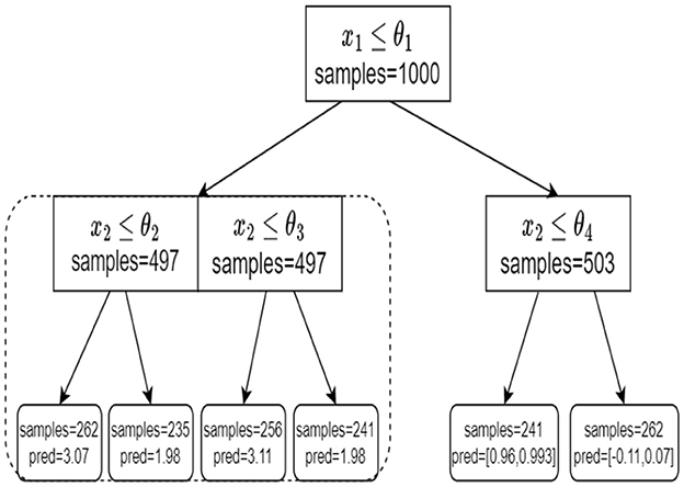
Figure 2. An example of our tree structure. At the root node, we split based on a single shared split. At the left child node, we treat each target independently. On the right node, we again split based on a single shared split.

3.2 Splitting criterion and evaluation

Naturally, one of the inherent challenges of our suggested method is to assess the performance of different splitting approaches (that is, MT vs. ST). Here, we follow the ALOOF framework (Section 2.3) and propose an estimator of the generalization error, based on cross-validation. Let $T={\left\{x_i,y_i\right\}}_{i=1}^m$ be a set observations in a given node. For simplicity of the presentation, we first assume a regression problem where y ∈ ℝ^d. Let T_tr and T_val be a partitioning of T into train and validation sets, respectively. Let j be an examined feature. Let $s_j^{*}$ be the optimal split value of the j^th feature over the train set. That is, $s_j^{*}$ is the argmin of Equation (4) over the set of observations T_tr, while the corresponding loss is $\mathcal{L}(s_j^{*})$. We repeat this process for K non-overlapping partitioning of T to obtain K values of $\mathcal{L}(s_j^{*})$. Finally, we average these K results, similarly to a classical K-fold CV scheme. We denote the resulting average as

$\begin{array}{ll}\begin{array}{c}G{E}_{MT}(j)=\frac{1}{K}{\displaystyle \sum _{k=1}^K}{\mathcal{L}}^{(k)}(s_j^{*})\end{array}& (5)\end{array}$

where ${\mathcal{L}}^{(k)}(s_j^{*})$ is the loss of the k^th fold, as described above.

Next, we would like to estimate the generalization error of the ST splits. Here, we repeat the same process, but for every target independently. That is, for the r^th target and the j^th feature, we define K partitioning to train and validations sets. Then, we find the best split, $s_{j,r}^{*}$ over the train-set (following Equation 1), and evaluate its performance on the validation set. We repeat this process K times and average the results to obtain (Equation 6)

$\begin{array}{ll}\begin{array}{c}G{E}_{ST}(j,r)=\frac{1}{K}{\displaystyle \sum _{k=1}^K}{\mathcal{L}}^{(k)}(s_{j,r}^{*})\end{array}& (6)\end{array}$

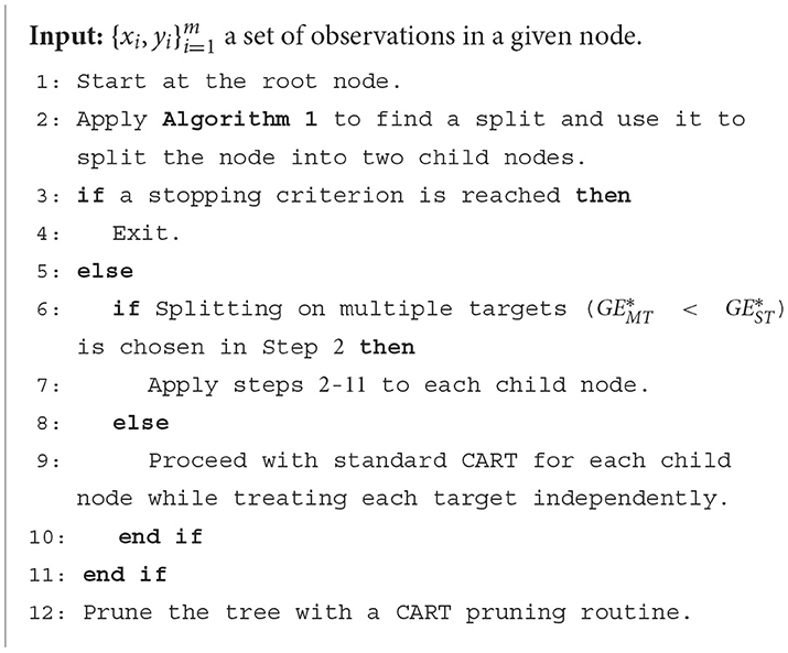
where here ${\mathcal{L}}^{(k)}(s_{j,r}^{*})$ is the argmin of Equation (1) over the train-set, for the r^th target. Finally, we compare the optimal splitting choice when treating all targets simultaneously, $G{E}_{MT}^{*}={min}_{j}G{E}_{MT}(j)$ and treating each target independently, $G{E}_{ST}^{*}=\sum _{r=1}^d{min}_{j}G{E}_{ST}(j,r)$. Algorithm 1 summarizes our proposed cross-validated splitting criterion. We continue the tree training process with the approach that yields the lower estimated generalization error. Specifically. if MT obtains a better result we proceed with a single shared split and repeat the process above for each of its child nodes. On the other hand, if ST is chosen we seek the optimal split for each of the d targets and proceed with a standard CART tree for each of the child nodes. We perform a no-regret tree-growing process, as previously described.

Algorithm 1

Algorithm 1. Comparing MT and ST.

Cross-validation is a widely used approach for estimating the generalization capabilities of a predictive model. Specifically, in K-fold CV, the original sample is randomly partitioned into K equal-sized sub-samples. This allows all available information to be incorporated into the model training process, ensuring that no unique information is overlooked in the validation set. K-fold CV requires a choice of K, but it is unclear which value should be used. With ten-fold CV, the prediction error estimate is almost unbiased (Simon, 2007), so K = 10 is a reasonable off-the-shelf choice. Hence, we use the above throughout our experiments.

Finally, we need to consider a stopping criterion. For simplicity, we apply the popular CART grow-then-prune methodology. This approach involves initially growing a large tree and subsequently pruning it to achieve its favorable size through cross-validation. A pseudo-code of our proposed method is provided in Algorithm 2.

Algorithm 2

Algorithm 2. Our proposed method.

Although we focus our attention to regression trees, our proposed method can be easily applied to classification problems. Specifically, the only modification required is to replace the squared error with the Gini index (Equation 2). In fact, the Gini index is closely related to the squared error if we utilize with 0 − 1 coding for the classes (Painsky and Rosset, 2016).

3.3 Computational complexity

Having discussed the main components of our proposed framework, we turn to its computational complexity. In regression problems, CART first sorts the n observation pairs according to their feature values and determines a cut that minimizes the loss on both sides of the cut. By scanning along this list, O(n) operations are required, resulting in an overall complexity of O(n·log(n)) due to sorting. As previously noted, seeking a single shared split only extends the loss function, leading to the same complexity. On the other hand, seeking d separate splits requires d times CART complexity. Therefore, the overall computational load of our proposed method is O(k·d·n′·log(n′)), where n′ is the size of the train-set, n′ = (k−1)n/k. For classification, the only adjustment required is the replacement of the loss criterion. Hence, the computational complexity remains unaltered.

4 Experiments

Let us now demonstrate our proposed method in a series of synthetic and real worlds experiments.

4.1 Synthetic experiments

We begin with an illustration of our proposed method in a series of synthetic experiments. In the first experiment we draw 600 observations from two features and d targets, ${\left\{x_{i1},x_{i2},y_{i1},\dots y_{id}\right\}}_{i=1}^n$. We define X_ij ~ U(−10, 10) and r^th target depends on the two features X₁, X₂ as follows.

$Y_r=\{\begin{array}{ll}{ϵ}_r,\hfill & \text{if }{X}_1>{\alpha }_r\text{ and }{X}_2>{\alpha }_r\hfill \\ 1+{ϵ}_r,\hfill & \text{if }{X}_1>{\alpha }_r\text{ and }{X}_2<{\alpha }_r\hfill \\ 2+{ϵ}_r,\hfill & \text{if }{X}_1<{\alpha }_r\text{ and }{X}_2>{\alpha }_r\hfill \\ 3+{ϵ}_r,\hfill & \text{if }{X}_1<{\alpha }_r\text{ and }{X}_2<{\alpha }_r\hfill \end{array}$

where ϵ_r ~ N(0, 1) i.i.d and α_r is a predefined parameter. Note that α_r determines the dependence between the features and the response variables. Further, notice that by choosing the α_r's very close to each other we get that the response variables are very correlated. Hence, in our experiments, we also use α_r as a parameter that controls the strength of the interaction between the response variables. The observations are split into 80% observations for the train-set and 20% for the test-set. We train the studied scheme on the train-set and evaluate the mean squared error (MSE) on the test-set. We further evaluate the ST and MRT as basic benchmarks. We repeat this process 500 times and report the averaged results.

First, we set d = 2 which corresponds to two response variables. for Y₁ we set α₁ = 0 and for Y₂ we consider different values of α₂. As mentioned above, small values of α₂ correspond to a greater correlation between the response variables. In this case, we expect MRT to be preferable. As α₂ increases, the response variables become less related, so ST is the preferable choice. Figure 3 shows that our proposed method successfully tracks the preferred approach in both cases. Specifically, for smaller α₂ we obtain a single tree with typically two levels, corresponding to the four possible outputs of the response variables. As α₂ increases we typically obtain two separate trees, where each tree corresponds to the four (different) outputs of each target. Next, we examine the effect of the number of response variables d. We set the values of α's to zero for each response variable, indicating that the response variables are derived from the same model and are strongly dependent. Figure 4 demonstrates the resulting MSE as the number of response variables increases. The upper curve corresponds the ST approach, which is agnostic to the number of response variables and the underlying models. The lower curve corresponds to the MRT approach, which demonstrates superior performance as the number of response variables increases due to their strong correlation. The middle curve is our proposed method, which successfully tracks the preferred MRT approach and enhances its accuracy as the number of response variables grows. Once again, our proposed method typically outputs a single tree with four output level, corresponding to α = 0 as desired.

Figure 3

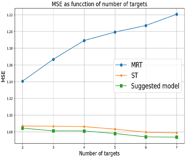
Figure 3. Synthetic experiment with two features and two response variables from the models are described in the text. The parameter α₁ is set to zero and different values of α₂ are evaluated.

Figure 4

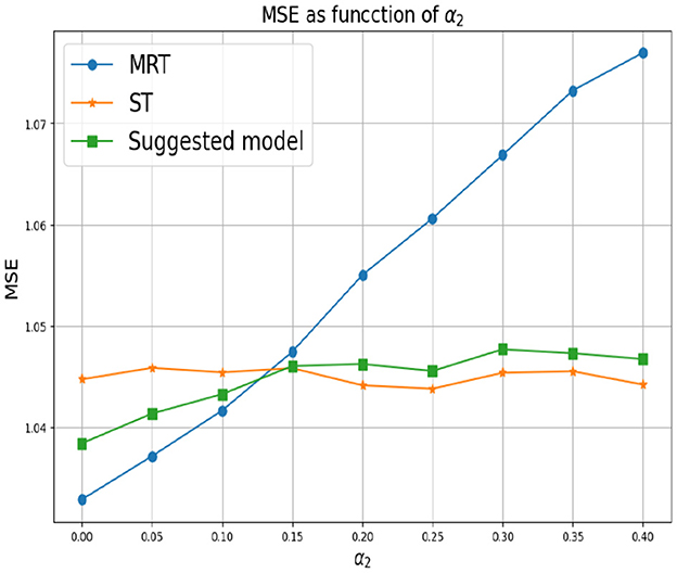
Figure 4. Synthetic experiment with two features. The parameters α_r are set to zero.

In the third experiment, the α_r's are arbitrarily chosen. This means that the response variables are derived from different models and there is an unknown dependence between them. Figure 5 summarizes the results we obtain. Here, MRT demonstrates a reduction in performance as the number of response variables increases. This decline can be explained by MRT attempting to exploit non-existent dependencies. This adverse effect becomes more pronounced as the number of response variables increased. As in the previous experiment, the ST approach at the bottom is agnostic to the number of response variables. However, it achieves superior performance in this setup, as the responses are (more likely) uncorrelated. Once again, our proposed method successfully tracks the favorable approach.

Figure 5

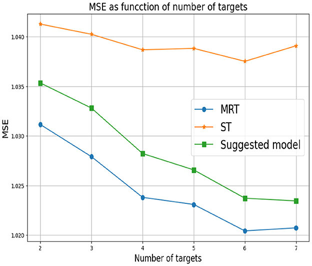
Figure 5. Synthetic experiment with two features. The parameters α_r are randomly drawn.

4.2 Real world experiments

We now turn to a real-world comparative study. Here, we not only demonstrate our approach in different setups but also compare it to additional alternatives. In the following experiments, we compare our proposed method with the standard ST and MRT schemes as above. In addition, we evaluate a model selection approach which utilizes CV to identify the best model among the two (that is, chooses between ST and MRT). We denote this scheme as ST/MRT. Furthermore, we implement RC/CC and SST/SBR (for regression and classification problems, respectively), with CART as a base model. See Section 2.1.1 for a detailed discussion. We also compare our proposed method with clustering trees (Breskvar et al., 2018) and deep tree-ensembles (DTE) (Nakano et al., 2022). Specifically, we apply the ROS-based methods in Breskvar et al. (2018) and the three deep forest schemes proposed by Nakano et al. (2022), denoted as X TE, X OS and X TE OS. Additional tree-based MTL methods are omitted as they focus on different merits (Piccart et al., 2008), or do not offer a publicly available implementation (and are too complicated to implement and tune) (Suzuki et al., 2001; Basgalupp et al., 2021). In addition, we increase the scope of our study and consider a Gradient Boosting (GB) framework (Friedman, 2001). That is, we implement a GB framework where the sub-learners are either MT, ST, or our proposed method. As the common practice, we implement GB with tree models and refrain from complex sub-learners (such as SST/SBR and RC/CC).

MTL has been extensively studied over the years, with several publicly available datasets. In the following, we briefly describe them and summarize their main properties. All these datasets are publicly available on openML² and Kaggle.³ In the Scpf dataset, we predict three targets that represent the number of views, clicks, and comments that have been collected from US major cities (Oakland, Richmond, New Haven, and Chicago). The dataset includes seven features such as the number of days the issue stayed online, the source of the issue (e.g., android, iPhone, remote API), the issue type (e.g., graffiti, pothole, trash), geographical coordinates of the issue, the city it was published from, and the distance from the city center. All multi-valued nominal variables were converted to binary, and rare binary variables (<1 of the cases) were removed. The focus of the Concrete Slump dataset (Yeh, 2007) is to predict the values of three concrete properties, namely slump, flow, and compressive strength, based on the composition of seven concrete ingredients, which include cement, fly ash, blast furnace slag, water, superplasticizer, coarse aggregate, and fine aggregate. The Jura dataset (Goovaerts, 1997) comprises measurements of seven heavy metals (cadmium, cobalt, chromium, copper, nickel, lead, and zinc) taken from locations in the topsoil of the Swiss Jura region. Each location's type of land use (Forest, Pasture, Meadow, Tillage) and rock type (Argovian, Kimmeridgian, Sequanian, Portlandian, Quaternary) were also recorded. The study focuses on predicting the concentration of three more expensive-to-measure metals (primary variables) using cheaper-to-sample metals (secondary variables). The response variables are cadmium, copper, and lead, while the remaining metals, land use type, rock type, and location coordinates serve as predictive features. Overall we utilize 1,515 features for prediction. Finally, the E-Commerce dataset comprises transaction records spanning the period from March to August 2018. The dataset contains several features, including the customer's ID, the category name, and the grand total, which represents the amount of money spent on each transaction. Prior to analysis, we preprocessed these features to create a new dataset, where each column represents a specific category and each row corresponds to a specific customer and the amount of spending on each category. We focus on “Mobiles & Tablets” and “Beauty & Grooming” as response variables. Consequently, the remaining 1,414 categories are treated as features in our analysis. Moreover, we analyze only those customers who had made purchases in a minimum of nine categories, to avoid the issue of sparse data. Furthermore, we examine our proposed method for classification. Specifically, we convert SCPF and E-Commerce to two-class classification problems by comparing their target values with their medians. In addition to the above, we study several benchmark datasets which are popular in the MTL literature. Their detailed descriptions are provided in Melki et al. (2017); Breskvar et al. (2018); Nakano et al. (2022), for brevity.

To evaluate the performance of the suggested method, we use MSE for regression and 0 − 1 loss for classification (Painsky, 2023). For GB we utilize 50 trees and limit their complexity by defining the minimum number of observations in the trees' terminal nodes to be 0.05·n. To ensure that our results are robust and are not influenced by the particular random partitioning of the data we apply standard ten-fold CV. It is important to emphasize that for each dataset, different targets may have a different scale. This leads to bias toward large scale targets. To overcome this difficulty, we normalize the targets accordingly.

Tables 1, 2 summarize the results we achieve for a single tree and an ensemble of models, respectively. For each experiment we report the averaged merit and its corresponding standard deviation in parenthesis. For each dataset, we mark (with a bold font) the method that achieves the best averaged performance. As we can see, our proposed method demonstrates superior accuracy for a single tree, while the difference is less evident with ensembles. This highlights the well-known advantage of using ensemble methods over a single tree, as they can mitigate the limitations of a single tree. Nevertheless, we also observe an evident improvement in the ensemble setup. To validate the statistical significance of our results, we apply a standard sign test (Demšar, 2006) between our proposed method and each of the alternatives. Specifically, we count the number of datasets in which our proposed method defeats each alternative scheme. Then, we test the null hypothesis that both methods perform equally well. We report the corresponding p-values for each alternative method. For single tree models we obtain p-values of 0.0014, 0.0195, 0.0058 when tested against ST, MRT and ST/MRT, respectively. These results imply that even with an appropriate multiplicity correction for three hypotheses, our proposed method is favorable with a statistical significance level of 0.0585. For ensemble models we obtain p-values of 0.0005, 0.0005, 0.0195, 0.0058, 0.0058, 0.0058, 0.0541, and 0.0195 when tested against SST/SBR, RC/CC, X TE, X OS, X TE OS, GB-ST, GB-MRT and GB-ST/MRT, respectively. Once again, we observe relatively low p-values which emphasize the validity of our results. Yet, these findings are less significant (after appropriate multiplicity correction), due to the greater number of alternative methods. In addition, we compare our proposed method to Breskvar et al. (2018), who focused on the aRMMSE measure (see Equation 5 in Breskvar et al., 2018). We repeat the experiments above and evaluate the aRMMSE for the last four datasets in Table 2, which were also studied in Breskvar et al. (2018). Our proposed method outperforms (Breskvar et al., 2018) in all of these datasets. To conclude, our results introduce favorable results over the alternative schemes, where the advantage is more evident in the more interpretable single tree setup.

Table 1

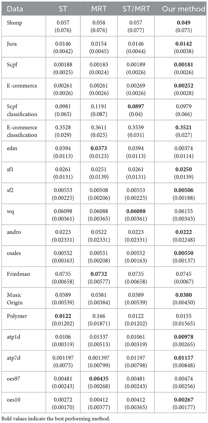
Table 1. Real-world data experiments non-ensembles.

Table 2

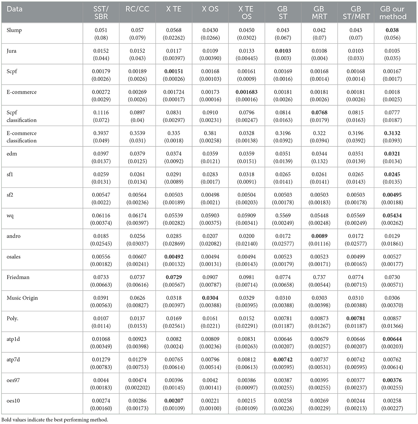
Table 2. Real-world data experiments—ensembles.

Finally, we evaluate and compare the execution time of the studied methods. Our proposed method takes ~2-3 times more to apply, on the average, then the traditional CART (that is, without ensembles). The reason that the computational load is less than a factor of ten (as one may expect from our worst-case analysis in Section 3.3) is quite straightforward. Our proposed method begins with a 10-fold CV in each level of the tree. However, once we observe that independent trees become favorable (in terms of expected generalization error), we continue the tree construction with traditional CART (see Step 9 of Algorithm 2).

5 Conclusions

In this work we propose a novel tree-based model for MTL. Our suggested framework utilizes the advantages of ST and MRT as we introduce a hybrid scheme of joint and separate splits. By adopting a CV framework for selecting the best approach at each node, we minimize the (estimated) generalization error to avoid overfitting and improve out-of-sample performance. We demonstrate our suggested approach in synthetic and real world experiments, showing preferable merits over alternatives.

Our work emphasizes the importance of carefully considering the trade-offs between joint and separate modeling when designing MTL methods. By identifying the strengths and weaknesses of both approaches and combining them in an innovative way, we achieve results that surpass those of both decision tree and gradient boosting methods. These findings have important implications for the development of more robust and versatile machine learning algorithms. Our method offers a promising solution to the challenge of MTL. It provides an effective approach to optimize performance while maintaining interpretability, critical factors for practical applications.

Data availability statement

Publicly available datasets were analyzed in this study. The datasets can be found in the OpenML and/or Kaggle repositories, and can be accessed via the following links: https://www.openml.org/search?type=data&sort=runs&id=41555&status=active; https://www.openml.org/search?type=data&sort=runs&id=41558&status=active; https://www.openml.org/search?type=data&status=active&id=41554&sort=runs; https://www.kaggle.com/datasets/zusmani/pakistans-largest-ecommerce-dataset.

Author contributions

YN: Data curation, Methodology, Software, Validation, Writing – original draft. AP: Conceptualization, Formal analysis, Funding acquisition, Investigation, Methodology, Project administration, Resources, Supervision, Validation, Writing – review & editing.

Funding

The author(s) declare financial support was received for the research, authorship, and/or publication of this article. This research was supported by the Israel Science Foundation grant number 963/21.

Conflict of interest

The authors declare that the research was conducted in the absence of any commercial or financial relationships that could be construed as a potential conflict of interest.

Publisher's note

All claims expressed in this article are solely those of the authors and do not necessarily represent those of their affiliated organizations, or those of the publisher, the editors and the reviewers. Any product that may be evaluated in this article, or claim that may be made by its manufacturer, is not guaranteed or endorsed by the publisher.

Footnotes

1. ^ https://github.com/a4566201/-Cross-validated-Tree-Based-Models-for-Multi-target-Learning

2. ^ https://www.openml.org/

3. ^ https://www.kaggle.com/

References

Adıyeke, E., and Baydoǧan, M. G. (2020). The benefits of target relations: a comparison of multitask extensions and classifier chains. Pattern Recognit. 107:107507. doi: 10.1016/j.patcog.2020.107507

Crossref Full Text | Google Scholar

Alves, A. H. R., and Cerri, R. (2022). “A two-step model for drug-target interaction prediction with predictive bi-clustering trees and xgboost,” in 2022 International Joint Conference on Neural Networks (IJCNN) (IEEE), 1–8.

Google Scholar

Appice, A., and Džeroski, S. (2007). “Stepwise induction of multi-target model trees,” in European Conference on Machine Learning (Springer), 502–509.

Google Scholar

Basgalupp, M., Cerri, R., Schietgat, L., Triguero, I., and Vens, C. (2021). Beyond global and local multi-target learning. Inf. Sci. 579:508–524. doi: 10.1016/j.ins.2021.08.022

Crossref Full Text | Google Scholar

Breiman, L., and Friedman, J. H. (1997). Predicting multivariate responses in multiple linear regression. J. R. Stat. Soc. Ser. B 59, 3–54. doi: 10.1111/1467-9868.00054

Crossref Full Text | Google Scholar

Breskvar, M., Kocev, D., and Džeroski, S. (2018). Ensembles for multi-target regression with random output selections. Mach. Learn. 107, 1673–1709. doi: 10.1007/s10994-018-5744-y

Crossref Full Text | Google Scholar

Brown, P. J., and Zidek, J. V. (1980). Adaptive multivariate ridge regression. Ann. Stat. 8, 64–74. doi: 10.1214/aos/1176344891

Crossref Full Text | Google Scholar

Burnham, A. J., MacGregor, J. F., and Viveros, R. (1999). Latent variable multivariate regression modeling. Chemometr. Intell. Lab. Syst. 48, 167–180. doi: 10.1016/S0169-7439(99)00018-0

Crossref Full Text | Google Scholar

De'Ath, G. (2002). Multivariate regression trees: a new technique for modeling species-environment relationships. Ecology 83, 1105–1117. doi: 10.1890/0012-9658(2002)083[1105:MRTANT]2.0.CO;2

Crossref Full Text | Google Scholar

Demšar, J. (2006). Statistical comparisons of classifiers over multiple data sets. J. Mach. Learn. Res. 7, 1–30.

Google Scholar

Evgeniou, T., and Pontil, M. (2004). “Regularized multi-task learning,” in Proceedings of the Tenth ACM SIGKDD International Conference on Knowledge Discovery and Data Mining, 109–117.

Google Scholar

Friedman, J. H. (2001). Greedy function approximation: a gradient boosting machine. Ann. Stat. 29, 1189–1232. doi: 10.1214/aos/1013203451

Crossref Full Text | Google Scholar

Ghosn, J., and Bengio, Y. (1996). Multi-task learning for stock selection. Adv. Neural Inf. Process. Syst. 9.

Google Scholar

Godbole, S., and Sarawagi, S. (2004). “Discriminative methods for multi-labeled classification,” in Pacific-Asia Conference on Knowledge Discovery and Data Mining (Springer), 22–30.

Google Scholar

Goovaerts, P. (1997). Geostatistics for Natural Resources Evaluation. Oxford: Oxford University Press on Demand.

Google Scholar

Izenman, A. J. (1975). Reduced-rank regression for the multivariate linear model. J. Multivar. Anal. 5, 248–264. doi: 10.1016/0047-259X(75)90042-1

Crossref Full Text | Google Scholar

Ji, S., Tang, L., Yu, S., and Ye, J. (2008). “Extracting shared subspace for multi-label classification,” in Proceedings of the 14th ACM SIGKDD International Conference on Knowledge Discovery and Data Mining, 381–389.

Google Scholar

Kocev, D., Džeroski, S., White, M. D., Newell, G. R., and Griffioen, P. (2009). Using single-and multi-target regression trees and ensembles to model a compound index of vegetation condition. Ecol. Modell. 220, 1159–1168. doi: 10.1016/j.ecolmodel.2009.01.037

Crossref Full Text | Google Scholar

Li, B., Friedman, J., Olshen, R., and Stone, C. (1984). Classification and regression trees (cart). Biometrics 40, 358–361. doi: 10.2307/2530946

Crossref Full Text | Google Scholar

Liu, G., Lin, Z., and Yu, Y. (2009). Multi-output regression on the output manifold. Pattern Recognit. 42, 2737–2743. doi: 10.1016/j.patcog.2009.05.001

Crossref Full Text | Google Scholar

Melki, G., Cano, A., Kecman, V., and Ventura, S. (2017). Multi-target support vector regression via correlation regressor chains. Inf. Sci. 415, 53–69. doi: 10.1016/j.ins.2017.06.017

Crossref Full Text | Google Scholar

Michelucci, U., and Venturini, F. (2019). Multi-task learning for multi-dimensional regression: application to luminescence sensing. Appl. Sci. 9:4748. doi: 10.3390/app9224748

Crossref Full Text | Google Scholar

Nakano, F. K., Pliakos, K., and Vens, C. (2022). Deep tree-ensembles for multi-output prediction. Pattern Recognit. 121:108211. doi: 10.1016/j.patcog.2021.108211

Crossref Full Text | Google Scholar

Osojnik, A., Džeroski, S., and Kocev, D. (2016). “Option predictive clustering trees for multi-target regression,” in Discovery Science: 19th International Conference, DS 2016, Bari, Italy, October 19-21, 2016, Proceedings 19 (Springer), 118–133.

Google Scholar

Painsky, A. (2023). “Quality assessment and evaluation criteria in supervised learning,” in Machine Learning for Data Science Handbook: Data Mining and Knowledge Discovery Handbook, eds L. Rokach, O. Maimon and E. Shmueli (Cham: Springer), 171–195.

Google Scholar

Painsky, A., and Rosset, S. (2016). Cross-validated variable selection in tree-based methods improves predictive performance. IEEE Trans. Pattern Anal. Mach. Intell. 39, 2142–2153. doi: 10.1109/TPAMI.2016.2636831

PubMed Abstract | Crossref Full Text | Google Scholar

Piccart, B., Struyf, J., and Blockeel, H. (2008). “Empirical asymmetric selective transfer in multi-objective decision trees,” in International Conference on Discovery Science (Springer), 64–75.

Google Scholar

Quinlan, J. R. (1986). Induction of decision trees. Mach. Learn. 1, 81–106. doi: 10.1007/BF00116251

Crossref Full Text | Google Scholar

Quinlan, J. R. (2004). Data mining tools see5 and c5. 0. Available online at: http://www.rulequest.com/see5-info.html (accessed February 2024).

Google Scholar

Quinlan, J. R. (2014). C4. 5: Programs for Machine Learning. San Mateo, CA: Elsevier.

Google Scholar

Read, J., Pfahringer, B., Holmes, G., and Frank, E. (2011). Classifier chains for multi-label classification. Mach. Learn. 85, 333–359. doi: 10.1007/s10994-011-5256-5

Crossref Full Text | Google Scholar

Salzberg, S. L. (1994). C4. 5: Programs for Machine Learning by j. ross quinlan. Burlington, MA: Morgan Kaufmann Publishers, Inc.

Google Scholar

Santos, B. Z., Nakano, F. K., Cerri, R., and Vens, C. (2021). “Predictive bi-clustering trees for hierarchical multi-label classification,” in Machine Learning and Knowledge Discovery in Databases: European Conference, ECML PKDD 2020, Ghent, Belgium, September 14-18, 2020, Proceedings, Part III (Springer), 701–718.

Google Scholar

Schapire, R. E., and Singer, Y. (2000). Boostexter: a boosting-based system for text categorization. Mach. Learn. 39, 135–168. doi: 10.1023/A:1007649029923

Crossref Full Text | Google Scholar

Simon, R. (2007). “Resampling strategies for model assessment and selection,” in Fundamentals of Data Mining in Genomics and Proteomics (Boston, MA: Springer), 173–186.

Google Scholar

Spyromitros-Xioufis, E., Tsoumakas, G., Groves, W., and Vlahavas, I. (2016). Multi-target regression via input space expansion: treating targets as inputs. Mach. Learn. 104, 55–98. doi: 10.1007/s10994-016-5546-z

Crossref Full Text | Google Scholar

Suzuki, E., Gotoh, M., and Choki, Y. (2001). “Bloomy decision tree for multi-objective classification,” in European Conference on Principles of Data Mining and Knowledge Discovery (Springer), 436–447.

Google Scholar

Weber, E. (1977). Kendall, m.: Multivariate analysis. charles griffin b co. ltd. london, high wycombe 1975. 210 s., 9 abb., 27 tab., 1 anhang, ?? 6,80. Biometr J. 19:309. doi: 10.1002/bimj.4710190413

Crossref Full Text | Google Scholar

Wu, X., Kumar, V., Ross Quinlan, J., Ghosh, J., Yang, Q., Motoda, H., et al. (2008). Top 10 algorithms in data mining. Knowl. Inf. Syst. 14, 1–37. doi: 10.1007/s10115-007-0114-2

Crossref Full Text | Google Scholar

Yao, Y., Shen, F., Xie, G., Liu, L., Zhu, F., Zhang, J., et al. (2020). Exploiting web images for multi-output classification: From category to subcategories. IEEE Transact. Neural Netw. Learn. Syst. 31, 2348–2360. doi: 10.1109/TNNLS.2020.2966644

PubMed Abstract | Crossref Full Text | Google Scholar

Yeh, I.-C. (2007). Modeling slump flow of concrete using second-order regressions and artificial neural networks. Cement Concr. Comp. 29, 474–480. doi: 10.1016/j.cemconcomp.2007.02.001

Crossref Full Text | Google Scholar