Establishing Multivariate Specification Regions for Incoming Raw Materials Using Projection to Latent Structure Models: Comparison Between Direct Mapping and Model Inversion

1 Introduction

For many manufacturing industries, reaching market standards in terms of product quality is a priority to ensure sales. Product quality is influenced by different factors, but one of the most important is the variability in raw material properties. If no corrective action is applied, these fluctuations propagate directly to final product quality. This is a real problem for many industries especially those processing bio-based materials using raw materials extracted from natural resources.

Ensuring good quality control may attenuate the impact of raw material variability. This can be performed in three ways: defining specifications for raw material properties, choosing adequate operating conditions, and characterizing final products for quality (Amsbary, 2013). A particular attention should be paid to the first as it deals directly with the source of the problem. Defining specifications and acceptance criteria for incoming lots of raw materials is key to achieve high and consistent quality final product. This is a useful tool to determine whether a lot of raw materials is processable, and indicates the risk of not reaching desired quality.

The main approach commonly used in the industry is to determine the acceptability of lots of raw materials based on a set of univariate specifications, past experiments, and/or the properties of the best suppliers (Duchesne and MacGregor, 2004). As the properties of any material are often highly correlated, univariate limits may lead to misclassification (De Smet, 1993; Duchesne and MacGregor, 2004). If the multiple univariate specifications are set large enough to accept all past good lots of raw materials, the risk of accepting bad quality lots increases. To mitigate this, univariate specification limits can be tightened to minimize acceptance of poor quality raw materials. However, this increases the rejection rate of good lots of materials, which typically leads to higher purchasing costs. Thus, the correlation structure between the raw material properties needs to be considered to minimize the risk of inadequate decisions. Establishing multivariate specification regions to select incoming lots of raw materials is a solution to this problem. The concept was first introduced by De Smet (1993). It consists of building a Projection to Latent Structures model first to relate the raw material properties to the final quality attributes. Then, each lot of raw materials is projected in the latent space of the PLS model. Its class assignment (e.g., good or bad quality) is inherited from the corresponding final product quality assessment, hence the name Direct Mapping (DM) approach. Finally, a boundary is established to discriminate the two classes by balancing type I and II errors or by minimizing one. The resulting region is then used to decide whether a new incoming lot of raw materials should be accepted or rejected.

As the impact of process control actions, changes in process operating conditions and disturbances on final product quality were not considered by De Smet (1993), Duchesne and MacGregor (2004) extended the previous approach. They proposed a framework for different scenarios based on how process variability affects final product quality, and its level of collinearity with raw material properties. The methods are illustrated using simulated and industrial data from a film blowing process (Duchesne and MacGregor, 2004). Tessier and Tarcy (2010) have also applied the technique in the context of the aluminum production.

Further improvements were then proposed. To increase the size of the dataset and to include more variations in the context of pharmaceutical process scale-up, García-Muñoz (2009) introduced a new step prior to the Duchesne and MacGregor technique to take into account data collected from multiple scales. Later, Azari et al. (2015) suggested using the Sequential Multi-Block PLS algorithm (SMB-PLS) instead of PLS as a more efficient method to establish multivariate specifications when raw material properties and process operating conditions are correlated. This approach allows to clearly identify the variation in raw material properties uncompensated by control actions. Finally, to establish specifications in situations where several different types of raw materials are used, MacGregor et al. (2016) have proposed a new approach based on Monte Carlo simulations to calculate the risk of accepting a new lot.

A similar concept to multivariate specifications called Design Space (DS) was introduced by the Internal Conference of Harmonization (2009) mainly for the pharmaceutical industry. The goal is to determine: “the multidimensional combination and interaction of input variables (e.g., material attributes and process parameters) that have been demonstrated to provided assurance of quality.” Essentially, the general objective of establishing a design space is to reduce product quality variability by design rather than by inspection techniques aiming at characterizing final product properties (MacGregor and Bruwer, 2008; Godoy et al., 2017). One main advantage of this approach is that modifications applied to the process or raw material variability within the DS are not considered as a change for the regulatory agencies as Food and Drug Administration (FDA) (ICH, 2009; Lawrence et al., 2014).

Even if the two concepts (raw material specifications and DS) aim at improving product quality control, differences exist between them. The DS is typically defined during the product development stage using raw material properties and process conditions simultaneously. Multivariate specifications, however, are built using larger sets of industrial historical data, and require that variability introduced by process variables be removed prior to defining the specification region. In addition, even if both concepts are based on PLS models, they use different mathematical approaches to determine the acceptance region. Defining a DS in latent space is mostly performed using PLS model inversion of a single desired quality attribute (Facco et al., 2015; Bano et al., 2017; Palací-López et al., 2019) while, in the past, multivariate specification regions were obtained using direct mapping of final product quality based on several correlated attributes. As suggest by Garcia-Muñoz et al. (2010), the inversion technique could be an alternative to DM for developing raw material multivariate specifications. Applying PLS model inversion using multivariate product quality attributes was demonstrated by Jaeckle and MacGregor (1998) and Jaeckle and MacGregor (2000) in the context of product development problems.

The objective of this paper is to compare the two approaches for establishing multivariate specification regions, namely PLS model inversion and direct mapping, in terms of classification performance for a given application, and to determine their advantages and drawbacks. It also shows how to establish multivariate specification regions by PLS inversion for a multivariate set of quality attributes, and assess the influence of different levels of correlation between them for both techniques. Such a comparison for one or multiple quality attributes has not been attempted in the past, to the best knowledge of the authors. The proposed paper should be considered as a guide to support the development of multivariate specifications using the most appropriate technique for a given application.

This work is quite ambitious since many scenarios need to be considered and several decisions had to be made to ensure a fair comparison. First, simulated data is used to allow multiple scenarios to be generated. A simple model involving four raw material properties and two final product quality attributes was developed to facilitate the comparisons and interpretations. The shape of the final product quality acceptance region was selected to be elliptical to reflect the correlation structure between the quality attributes. When building the PLS models between final product quality attributes and raw material properties, the number of components retained in both approaches is chosen as that maximizing classification performance for the PLS inversion approach. This choice was made to avoid introducing biases in the comparison since the direct mapping approach has more flexibility. For each combination of final product quality attributes, a single PLS model is built and used to define the specification regions with both approaches. Finally, the classification performance is assessed without considering the uncertainty back propagation (Bano et al., 2017).

The paper is organized as follows. First, the simulator used to generate the datasets is presented. Then, the proposed methodology is exposed. The section includes a brief description of PLS regression, how to establish multivariate specifications using direct mapping and PLS inversion, as well as the classification metrics used to calculate classification performance. The results are then presented and discussed. Thereafter, the main conclusions are drawn.

2 Dataset Generation

Within the scope of the study, to simplify the comparison between the two techniques, multivariate specifications are developed under the hypothesis that process variables do not influence the quality of the product (i.e., the process is under control). However, how to cope with process variations in establishing multivariate specifications and design spaces was already extensively studied (Duchesne and MacGregor, 2004; Azari et al., 2015; Facco et al., 2015; MacGregor et al., 2016). The comparative analysis proposed in this study is generic, and is applicable in scenarios where process variations significantly affect product quality. Hence, in this study, only two blocks of data X (N×M) and Y (N×K) are involved when building PLS models. The first contains M raw material properties characterized in the laboratory or on-line using spectroscopy techniques, for instance, and the second K quality attributes of the final product collected for N observations or lots of raw materials. The data contained in these matrices are generated by simulations using analytical equations as described in the following subsection to facilitate the generation of combinations of y-variables spanning the full range of correlation. In addition, for the N observations included in the dataset, the quality of the final product is assigned to a class using a binary variable (i.e., good/bad quality) which is used to assess classification performance. The methods used to establish multivariate specification regions are then presented.

2.1 Simulated Process

The X-dataset is inspired from the model proposed by De Smet (1993). A total of four equations are used to generate variations in raw material properties:

$\begin{array}{c}{x}_1=22+h_1\end{array}(1)$

$\begin{array}{c}{x}_2=\sqrt{0.1+2h_2+3x_1}\end{array}(2)$

$\begin{array}{c}{x}_3=1.5+0.3x_1+0.5x_2+h_3\end{array}(3)$

$\begin{array}{c}{x}_4=12+0.5h_4\end{array}(4)$

where $h_i$ are random numbers following a standard normal distribution N(0,1). Correlation exists between properties 1–3 while the fourth is independent of the others.

For each lot of raw materials, i.e. an observation in X, two quality attributes are calculated using the following equation:

$\begin{array}{c}{y}_j={\displaystyle \sum }_{i=1}^4{k}_{i,j}{g}_{i,j}{x}_i\end{array}(5)$

and the values are stored in the Y matrix. The binary variables $k_{i,j}$ determine if the $i^{th}$raw material property affects the $j^{th}$ quality attribute while $g_{i,j}$ consists of random integers between −5 and 5. These were used to generate different magnitude for the effect of each x-variable on the y-variables. As the objective of this article is to compare the performance of two approaches for defining specification regions under different levels of correlation between both y-variables, the same X dataset is used throughout the analysis to generate different combinations of y-variables by changing parameters $k_{i,j}$ and $g_{i,j}$. When the product of these two parameters results in similar values for both y-variables, a high level of correlation is obtained. Conversely, very different values for this product leads to a low correlation. The span of different levels of correlations is owing to the random values generated for $g_{i,j}$. It should be noted that each combination is obtained randomly and not by smoothly increasing the correlation level between the y-variables.

Noise is added to all variables. The measured values $y_{m,j}$ and $x_{m,i}$ are obtained using the following equations:

$\begin{array}{c}{y}_{m,j}=y_j+\left({\epsilon }_{y,j}{\overline{y}}_j\right)e_{y,j}\end{array}(6)$

$\begin{array}{c}{x}_{m,i}=x_i+\left({\epsilon }_{x,i}{\overline{x}}_i\right)e_{x,i}\end{array}(7)$

where $e_{y,j}\text{ and }{e}_{x,i}$represent the errors added to the y- and x-data. These random errors also follow a standard normal distribution N(0,1). Their magnitude is characterized by the error standard deviation set as a percentage $\epsilon$ of the mean $\overline{x}$ or $\overline{y}$ for each variable. In all simulations, noise was generated in the same way. The values of $\epsilon$ and $\overline{x}$ are presented in Table 1 while$\overline{y}$ are not shown since they vary from one dataset to another. The mean values are obtained using the calibration dataset which contained 500 observations.

TABLE 1

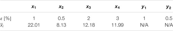
TABLE 1. Noise percentage and nominal signal values.

In addition to the calibration set, two other datasets are generated. The first is used to determine the number of PLS components needed while the classification performance of the specification regions is assessed using the second. Each of these datasets contains 10,000 observations. This number was selected in such a way that stable classification performance for each metric is obtained. Note that a large number of data points were generated as a mean to compare the direct mapping and inversion methods using a fair and sound statistical approach. However, both methods have already been demonstrated as effective on smaller datasets collected on simulated and industrial processes (Duchesne and MacGregor, 2004; Facco et al., 2015).

2.2 Definition of Product Acceptance

Establishing multivariate specification regions using a data-driven approach begins with identifying past lots of products of good and poor quality. This involves a product acceptance region in the Y-space. As the data used in this work are obtained from simulations, an indicator associated with the final quality of the product needs to be defined to identify good and bad products. The acceptance limit used in this study has an elliptical shape:

$\begin{array}{c}\left(\mathbf{y}-\overline{\mathbf{y}}\right){\mathbf{\Sigma }}_{\mathbf{y}}\left(\mathbf{y}-\overline{\mathbf{y}}\right)\text{′}\le \zeta \end{array}(8)$

where $\overline{\mathbf{y}}$ $(1\times K)$ is the vector containing the means of each y-variable, and ${\displaystyle {\Sigma }_y\left(K\times K\right)}$ is the y-covariance matrix. Parameter $\zeta$ is adjusted to specify the size of the region and to control the proportion of data assigned to good and bad quality. Once this parameter is selected, a binary variable was used to assign each observation to good and bad classes. In this work, $\zeta$ was chosen to ensure a proportion of good/bad products of 4:1. Even if the ratio of bad product is quite high compared to what is usually observed in industry, this choice was made to reduce the impact of class imbalance. There is no specific rule stating that a dataset should not be used as it is too imbalanced. However, in practice, ratios ranging from 2:1 to 10:1 are considered to be between marginally and modestly imbalanced (Weiss, 2013). Therefore, a choice was made to find a compromise between a realistic situation and balanced classes. When using industrial data, the ratio should be adjusted to obtain a more balanced dataset by oversampling the smallest class or under-sampling the most populated one (He and Garcia, 2009).

3 Methods

This section presents the direct mapping and PLS inversion-based approaches used to define multivariate specifications regions. As both techniques are based on PLS regression, a brief overview of this latent variable method is provided. Finally, the classification metrics used to quantify the performance are described.

3.1 Projection to Latent Structure Regression

Before building PLS models between X and Y, the data are mean-centered and scaled to unit variance. As the X and Y matrices contained collinear data, latent variable modelling techniques are suitable approaches. PLS regression is retained as it builds the best linear relationships between the X and Y while modelling the variability contained in both spaces.

Variability is extracted using a group of A orthogonal latent variables known as scores T ($N\times A)$. PLS regression is defined mathematically by the following set of equations:

$\begin{array}{c}\mathbf{X}=\widehat{\mathbf{X}}+\mathbf{E}=\mathbf{T}{\mathbf{P}}^{\prime }+\mathbf{E}\end{array}(9)$

$\begin{array}{c}\mathbf{Y}=\widehat{\mathbf{Y}}+\mathbf{F}=\mathbf{T}{\mathbf{C}}^{\prime }+\mathbf{F} \end{array}(10)$

$\begin{array}{c}\mathbf{T}=\mathbf{X}{\mathbf{W}}^{\ast }=\mathbf{XW}{\left({\mathbf{P}}^{\prime }\mathbf{W}\right)}^{-1}\end{array}(11)$

where E $(N\times M)$ and F $(N\times M)$ are the model residuals. C$\mathit{ }(K\times A)$ and P$\mathit{ }(M\times A)$ are the loadings of the Y and X spaces, respectively. The loadings and the score values are computed using the NIPALS algorithm (Wold et al., 2001). It also provides the weight matrices W$(M\times A)$ and W^∗$\mathit{ }(M\times A)$ allowing to make predictions of Y based on X.

Prior applying PLS to new X-data, it is important to ensure that they are consistent with historical data used to build the model. This is achieved by computing the squared prediction error SPEX and the Hotelling’s T², and verifying that they fall below their respective statistical limits. The SPEX is used to check consistency of the correlation structure of new data. It is defined as follows:

$\begin{array}{c}{\text{SPEX}}_{\text{i}}={\mathbf{e}}_{\mathbf{i}}{\mathbf{e}}_{\mathbf{i}}^{\prime }\end{array}(12)$

where ${\mathbf{e}}_i (1\times K)$ is the X-residual vector for the i^th observation:

$\begin{array}{c}{\mathbf{e}}_i={\mathbf{x}}_i-{\mathbf{t}}_{\text{i}}\mathbf{P}\end{array}(13)$

As the SPEX values follow approximately a ${\chi }^2$ distribution with $\frac{2m^2}{v}$ degrees of freedom (Nomikos and MacGregor, 1995), a (1-$\alpha$) upper control limit (UCL) can be obtained:

$\begin{array}{c}{\text{SPE}}_{\text{UCL}}=\frac{v}{2m}{\chi }_{\frac{2m^2}{v},\alpha }^2\end{array}(14)$

where v and m are respectively the variance and the SPE mean calculated during the model calibration.

The Hotelling’s T² is used to measure the distance of projected new observations from the origin of the latent variable space. It is typically used to confirm whether a new observation falls within the so-called knowledge space (KS). The KS represents the space spanned by historical data in the latent variable space of the PLS model. The T² value for the $i^{th}$ observation is obtained as follows:

$\begin{array}{c}{\text{T}}_{\text{i}}^2={\displaystyle \sum }_{a=1}^A{\left(\frac{t_{a,i}}{s_a}\right)}^2\end{array}(15)$

where $t_{a,i}$ is the score values obtained for the a^th component and $s_a$ its standard deviation calculated in calibration.

The T² values are known to follow a Fischer distribution approximately (Jackson and Edward, 1991). A (1-$\alpha )$ upper control limits as proposed by Weirda (Wierda, 1994) can be calculated using the number of points in the calibration dataset N and the number of components retained A using the following equation:

$\begin{array}{c}{\text{T}}_{\text{UCL}}^2=\frac{A\left(N^2-1\right)}{N\left(N-A\right)}{F}_{A,N-A,\alpha }\end{array}(16)$

where $F_{A,N-A,\alpha }$ is the value of the Fischer distribution for A and (N-A) degrees of freedom. This elliptical-shaped limit is typically drawn in the scores space. The length of each axis $r_a$ is equal to:

$\begin{array}{c}{r}_a=\sqrt{\frac{A\left(N^2-1\right)}{N\left(N-A\right)}{s}_a^2{F}_{A,N-A,\alpha }}\end{array}(17)$

which is deduced from Eq. 15 and Eq. 16.

One important step in the model development is to select the optimal number of components. The appropriate method depends on how the model will be used. If the objective is to build PLS models for making predictions, criteria such as cumulative predicted variance Q²Y or the root mean squared errors of prediction (RMSEP) in cross-validation or calculated on an external dataset should be used. For a classification problem, such as defining multivariate specification regions, the optimal number of components should be the one that maximizes the classification performance on an external dataset. Classification performance is obtained by using the accuracy as defined in a following section.

The same PLS model is used to establish multivariate specification regions using both DM and inversion techniques. The number of components maximizing classification performance may be different for both approaches, but a single value of A needs to be selected for the comparative study. As the direct mapping is based on a compromise between type I and type II errors, which is an additional degree of freedom compared to inversion, using direct mapping might introduce a bias when choosing the number of components. To overcome this issue, the number of components is determined by maximizing classification performance obtained with the inversion approach, and this number of components is also used for DM.

3.2 Direct Mapping Approach

Defining multivariate specifications using direct mapping is performed in two steps. First, a PLS model is built using the quantitative y-data. Second, the specification limit in the latent space is defined by mapping product quality in the scores space. In other words, the class assigned to the score values (i.e., good/bad) corresponds to that of the final product obtained for the same lot of raw materials. The goal is to define a region that allows the separation of the two classes. Note that the quality classes are only used to assess classification performance in the latent space and not for building discriminant PLS models (i.e., PLS-DA). The shape of the region is defined by the user. In this study, a similar shape as that of the product quality acceptance region is chosen for both methods. Since the limit in the Y-space is elliptical and the PLS model is linear, the region obtained in the score space by inversion is also elliptical. For this reason, the following elliptical-shaped specification region was selected for the DM approach:

$\begin{array}{c}\mathbf{t}\mathbf{\Lambda }{\mathbf{t}}^{\prime }\le \eta \end{array}(18)$

where Λ $(A\times A)$ is the score covariance matrix. The value of η is used to adjust the size of the elliptical region. The strategy used to select η depends on the context in which the specification will be used, and the consequence of each type of misclassification. One may prefer minimizing type I or type II error while another could seek a compromise between both. By definition, type I error represents a sample predicted as bad quality when it is good while a type II error is a sample of truly bad quality predicted as good. For this work, as there is no specific context or limitation, the value of η is chosen to be the one leading to the same percentage of type I and type II errors.

Prior to using the specified region for incoming new lots of raw materials, the correlation structure of each observation needs to be assessed to ensure the model validity for this lot. This is done by defining an upper control limit on SPEX during the PLS model calibration as discussed in the previous section. If a given lot violates the limit, it should be flagged as having an inconsistent correlation structure compared with historical data, and should be rejected unless it is desired to process it, and used it to update the model and/or improve the specification region definition.

3.3 Projection to Latent Structure Model Inversion

Alternatively, multivariate specification regions in the score space can be established by inverting the PLS model for each point lying on the final product quality acceptance limit. In other words, instead of adjusting a limit within the score space using product quality class assignments, the limit is propagated from the Y-space acceptance region using the model structure.

As the limit in the Y-space is elliptical in this study, its parametric equation is used to generate combinations of quality attributes $(y_1,y_2)$ lying on the ellipse to use for the inversion. The transformation for the matrix to the parametric equation is the following:

$\begin{array}{c}\left[{\mathbf{y}}_1,{\mathbf{y}}_2\right]=\mathbf{V}\sqrt{\mathbf{D}}\left[\cos \left(\mathbf{\theta }\right),\mathit{ }\sin \left(\mathbf{\theta }\right)\right]\end{array}(19)$

where D $(K\times K)$ is a diagonal matrix containing the eigenvalues of $\zeta {\mathbf{\Sigma }}_y$ and V $(K\times K)$ the corresponding eigenvectors while $\mathbf{\theta }$ contains value between 0 and $2\pi$.

For each combination $(y_1,y_2)$ which is named ${\mathbf{y}}_{\mathit{des}}$ ($1\times K$), the PLS inversion method proposed by Jaeckle and MacGregor (1998) and Jaeckle and MacGregor (2000) allows calculating the corresponding score vector ${\mathbf{t}}_{\mathit{des}} (1\times A)$. Computations begin with the PLS model equation for the Y-space:

$\begin{array}{c}{\mathbf{y}}_{\mathit{des}}={\mathbf{t}}_{\mathit{des}}{\mathbf{C}}^{\prime }\end{array}(20)$

where the dimensions of the loading matrix C yields three possible cases depending upon the number of PLS components A and the number of y-variables K, as described in the following subsections.

3.3.1 Case 1: A = K

This case is the simplest one since there is a unique solution (i.e., number of equations equal to number of unknown parameters). As C is a square matrix, solving for ${\mathbf{t}}_{\mathit{des}}$ from Eq. 20 yields the following result:

$\begin{array}{c}{\mathbf{t}}_{\mathit{des}}={\mathbf{y}}_{\mathit{des}}{\left({\mathbf{C}}^{\prime }\mathbf{C}\right)}^{-1}= {\mathbf{y}}_{\mathit{des}}{\left({\mathbf{C}}^{\prime }\right)}^{-1}\end{array}(21)$

which directly provides the score vector associated with a combination of y-variables lying on the product acceptance region. The two terms are equivalent since C is a square matrix.

3.3.2 Case 2: A < K

In this case, since the number of unknown parameters is lower than the number of equations, there is no solution. As the matrix C is not square, to obtain ${\mathbf{t}}_{\mathit{des}}$ from Eq. 20 a right inverse is used. The resulting equation is the following:

$\begin{array}{c}{\mathbf{t}}_{\mathit{des}}=\mathbf{yC}{\left({\mathbf{C}}^{\prime }\mathbf{C}\right)}^{-1}\end{array}(22)$

In fact, the solution is the result of an ordinary least squares prediction between y and C where the prediction error of y is minimized (Jaeckle, 1998).

3.3.3 Case 3: A > K

For DS estimation, this case is the one that happens the most frequently (Facco et al., 2015; Palací-López et al., 2019). Since there are more unknown parameters than equations, the number of solutions is infinite. To obtain all of the possible solutions, Jaeckle and MacGregor (1998), Jaeckle and MacGregor (2000) proposed the following approach. As ${\mathbf{C}}^{\prime }\mathbf{C}$ is singular, solving for ${\mathbf{t}}_{\mathit{des}}$ requires using the Moore-Penrose inverse. Prior to the inversion, Jaeckle and MacGregor (2000) suggested to transform the score vector t into two new matrices to facilitate proper scaling:

$\begin{array}{c}{\mathbf{y}}_{\mathit{des}}=\mathbf{t}{\mathbf{C}}^{\prime }= \mathbf{uS}{\mathbf{C}}^{\prime }\end{array}(23)$

where u $(1\times A)$ is an orthonormal vector and S $(A\times A)$ is a diagonal matrix where the diagonal values are equal to $\sqrt{{\mathbf{T}}^{\prime }\mathbf{T}}$ . Then, using the Moore-Penrose inverse for a combination of y-variables stored in ${\mathbf{y}}_{\mathit{des}}$, the predicted value ${\mathbf{t}}_{\mathit{pred}}$ is obtained:

$\begin{array}{c}{\mathbf{t}}_{\mathit{pred}}={\mathit{y}}_{\mathit{des}}{\left(\mathbf{C}{\mathbf{S}}^{\prime }\mathbf{S}{\mathbf{C}}^{\prime }\right)}^{-1}\mathbf{C}{\mathbf{S}}^{\prime }\mathbf{S}\end{array}(24)$

which is the solution that is the closest to the origin of the PLS model plane. The other possible solutions ${\mathbf{t}}_{\mathit{des}}$ are distributed along the null space:

$\begin{array}{c}{\mathbf{t}}_{\mathit{des}}={\mathbf{t}}_{\mathit{pred}}+{\mathbf{t}}_{\mathit{null}}\end{array}(25)$

where ${\mathbf{t}}_{\mathit{null}}$ spans an orthogonal subspace of $A-K$dimensions. To obtain ${\mathbf{t}}_{\mathit{null}}$ values, singular value decomposition is applied on $\mathbf{S}{\mathbf{C}}^{\text{′}}$ to extract the left singular vectors. Only the (A-K) vectors associated with null singular values are kept in matrix G₂$\mathit{ }(A\times \left(A-K\right))$. The ${\mathbf{t}}_{\mathit{null}}$ vector is then calculated as follows:

$\begin{array}{c}{\mathbf{t}}_{\mathit{null}}=\mathbf{\lambda }{\mathbf{G}}_2\mathit{\prime }\mathbf{S}\end{array}(26)$

by specifying a (A-K) vector of constants $\mathbf{\lambda }\left(1\times \left(\mathit{A}-\mathit{K}\right)\right)$ that represents a position along the null space.

As the specification region is defined using an infinite number of equations (i.e. one for each point of the ellipse in the y-space), determining whether an observation falls within the specification limits or not is not simple. Geometrical approaches such as triangularization or visual inspection of score plots when A < 4 are needed to determine the position of one observation towards the region. When A > 3, more complex manipulations and calculations are necessary to determine the position of the scores with respect to the specification limits. Hence, in this study, it was decided to limit the number of PLS components to A ≤ 3. Also, before projecting a new lot into the specification region, the same approach using the SPEX limit needs to be performed to ensure that the model is valid for new observations.

3.4 Classification Metrics

As the main objective of this study is to compare two methods for developing multivariate specification regions, metrics are needed to compare their classification performance. Five different metrics are considered. They are based on the elements of the confusion table, which is schematically represented in Figure 1A.

FIGURE 1

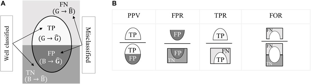
FIGURE 1. Schematic representation of the classification metrics: (A) confusion matrix (B) classification metrics.

The figure shows the relationship between the ground truth for good (G) and bad (B) final product, and the predicted class labels $\widehat{\text{G}}$ and $\widehat{\text{B}}$. In summary, a true positive TP is a good product well classified while false negative FN is a good product predicted as bad. On the other hand, a bad product which is misclassified is considered a false positive FP, and a true negative TN when it is well classified. It should be noted that FN and FP correspond to type I and II errors, respectively.

The first performance metric used is accuracy (ACC), which consists of the ratio of well-classified samples over the whole population:

$\begin{array}{c}\text{ACC}=\frac{\text{TP}+\text{TN}}{\text{TP}+\text{TN}+\text{FP}+\text{FN}}\end{array}(27)$

The next four metrics are shown in (Figure 1B) illustrated as the element of the confusion matrix. This allows a better visualization of the calculated ratios. Precision, also known as positive predictive value (PPV), is defined as:

$\begin{array}{c}\text{PPV}=\frac{\text{TP}}{\text{TP}+\text{FP}} \end{array}(28)$

which is the ratio of predicted good products to all the good observations. Recall, or true positive rate (TPR), is defined as follows:

$\begin{array}{c}\text{TPR}=\frac{\text{TP}}{\text{TP}+\text{FN}}\end{array}(29)$

It is the proportion of the well classified good product. False positive rate (FPR):

$\begin{array}{c}\text{FPR}=\frac{\text{FP}}{\text{FP}+\text{TN}}\end{array}(30)$

is used to quantify the percentage of misclassified bad products. The last metric is the false omission rate (FOR) which represents the percentage of errors made in assigning bad quality products to the right class:

$\begin{array}{c}\text{FOR}=\frac{\text{FN}}{\text{TN}+\text{FN}}\end{array}(31)$

4 Results and Discussion

The results are presented in three parts. First, a simple example considering a single quality attribute is shown to illustrate the methodologies, and to explain the main criteria used for comparing both techniques. Then, the impact of collinearity between the two quality attributes on the shape and size of the specification regions is presented. Finally, the main advantages and disadvantages of both techniques are highlighted based on the observations made during the analysis.

For ease of presentation, Table 2 summarizes all the information used to generate the different scenarios. The table is divided in three parts. First, the columns identified as Y-space definition show the values of the simulation model parameters selected for generating the datasets. This includes the coefficients $(k_i\times g_i)$ needed to define the y-variables, and the level of correlation between them, as well as the quality constant $\zeta$ that allows obtaining a 4:1 good/bad class ratio. The second part provides an overview of the PLS model performance in validation. The accuracy (ACC) obtained when inverting the model, which was used to choose the number of Latent Variables (LV) retained A, as well as the cumulative predicted explained variance Q²Y are shown in the table. The last part provides the values of the DM constant adjusting the size of the specification region, and the resulting percentage of type I and II error.

TABLE 2

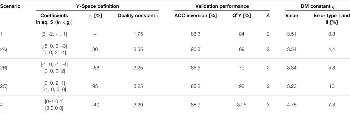
TABLE 2. Summary of the parameters involved in establishing specification regions with DM and PLS inversion, as well as some performance statistics for the different scenarios investigated.

4.1 Scenario 1–Illustration Using a Simple Example

The first scenario proposed is obtained by using one quality attribute. The output is simulated with all raw material properties affecting the quality attribute (i.e., $k_i\ne 0$) with a different value of $g_i$ for each x-variable as shown in Table 2. Then, the product quality acceptance zone is defined. Since the Y-space is univariate, the product acceptance region consists of lower and upper bounds using Eq. 8 where $\zeta$ = 1.75.

After mean-centering and scaling the data using the calibration dataset, the PLS model is built, and the number of components is selected to maximize classification accuracy for PLS inversion. Table 2 shows that an optimal accuracy of 88.3% is obtained using 2 components. The resulting model predicts 84% of the y-variance (Q²Y) based on the validation set. This model is then used to define the DM specification region by finding the value of $\eta$ that gives the same percentage of type I and type II errors. The obtained value of 3.51 leads to 8.8% of both types of errors.

At this point, both specification regions are defined and drawn in the latent space. For ease of visualization, Figure 2 shows a subsampling of the testing dataset where the proportion of each class is preserved. The solid black line represents the DM region obtained previously.

FIGURE 2

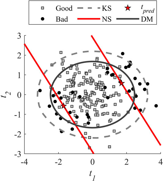
FIGURE 2. Score plot showing the multivariate specification regions obtained using both Direct Mapping and PLS Inversion for Scenario 1.

Since the number of components is higher than the number of quality attributes ($A>K)$, the specification region was determined using the inversion case 3 which considers the presence of a null space. The lower and upper y-limits are inverted to obtain the corresponding $t_{pred}$ values represented by red stars. The null-space (NS) is calculated and shown by the solid red line. Thus, all score values falling between these two lines are associated with good quality final product as per the inversion approach. However, this region is opened which may lead to misclassification as the predicted score values outside the knowledge space (KS) extrapolate. Therefore, the solution is constrained by the 95% upper Hotelling’s T² limit as advocated in some papers (Tomba et al., 2012; Facco et al., 2015; Bano et al., 2017). The gray dash line represents the KS.

It is observed in Figure 2 that the DM is already included inside the KS. This was expected because, the DM ellipse is designed to discriminate the classes using the calibration dataset which is the same used to define the KS. In addition, the inversion seems slightly better compared to direct mapping. Better performance might have been obtained if another shape was chosen for DM regions (i.e., the shape is an additional degree of freedom for DM).

Based on these observations, the performance in classification is analyzed using the classification metrics described in section Classification Metrics. Three different specification regions are considered. The first is the region obtained with the inversion alone (NS). The second is the NS region constrained by the KS $\left(\text{NS}\cap \text{KS}\right)$. The third is the DM region.

For all the metrics, the performance obtained with PLS inversion approaches are quite similar except for the false omission rate that is higher when considering the KS limit. Constraining the region within the KS generates more good samples predicted as bad, which increase the number of FN as shown in Figure 2.

When comparing direct mapping and inversion coupled with KS, Figure 3 shows that the performance are better for inversion for all the metrics. A particular attention should be paid to FPR and FOR for the DM as the difference is higher compared to other metrics. For the FPR, it can be seen in Figure 2 that the edge of the ellipse allows accepting more lots of bad quality which is not the case for the inversion. The higher FOR metric is caused by the bounding of the region with the KS limit.

FIGURE 3

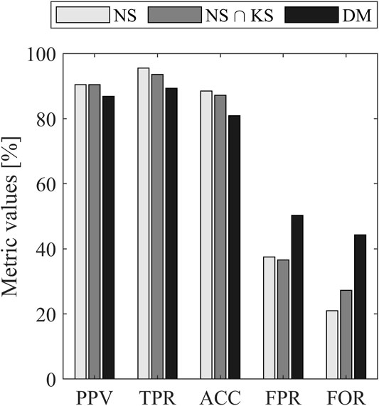
FIGURE 3. Classification performance metrics for Scenario 1.

Globally, Scenario 1 allowed to illustrate the methodology with a simple example using a univariate quality attribute. The basis is set to analyze more complex cases with multiple quality attributes. For the proposed example, the inversion is slightly better compared to direct mapping based on the five metrics. Also, the acceptance region is more restrictive for the direct mapping since its area is smaller compared to inversion. The performance might have been better if the shape of the DM regions would have been modified to exploit this additional degree of freedom.

4.2 Scenarios 2, 3 and 4: Impact of Collinearity Between Quality Attributes on the Specification Regions

The impact of collinearity between the two quality attributes is studied with respect to the three inversion cases (i.e.,$A<K$, $A>K$ and $A= K$). Initially, 400 combinations of two quality attributes were generated using the simulator (Eq. 5). For each of them, the number of components was chosen based on maximizing classification accuracy for PLS inversion. Figure 4 shows the number of y-combinations for the different levels of correlation, and the number of components retained when building the PLS model. Note that both negative and positive correlations were obtained, but the absolute value is shown in the figure.

FIGURE 4

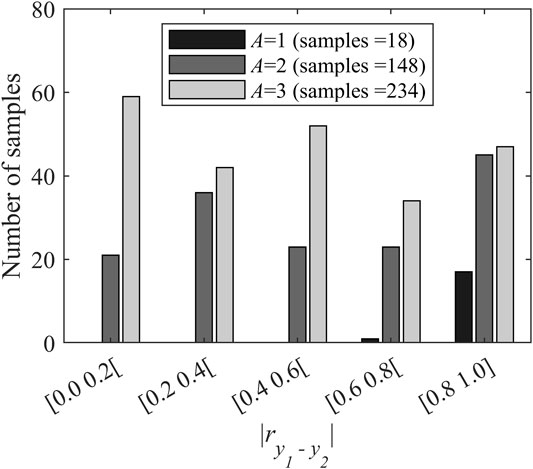
FIGURE 4. Distribution of the combinations of y-variables and the corresponding number of PLS components as a function of level of collinearity.

As it can be observed in Figure 4, 58.5% of the combinations require three components and they cover the full range of correlations. The samples associated with two components also spanned the entire range. This is not the case for the datasets where a single component is selected. Less than 5% of the combinations fall in this category and they concentrate in the zone of high levels of correlation i.e., with a value of $\left|r_{y_1-y_2}\right|$ greater than 80%. This was expected as when correlation coefficient tends toward unity, fewer components are needed since both y-variables are almost the same, and so is X.

It should be noted that the number of components retained depends strongly on the selected performance criteria. If another metric would have been selected or if the performance had been calculated using the direct mapping, the number of combinations associated with each inversion cases and their distribution relative to the level of correlation between both y-variables might have been different.

4.2.1 Scenario 2: Impact of Collinearity When A = K

In this scenario (involving inversion Case 1), the 148 combinations associated with A = 2 in Figure 4 are considered to analyze the impact of correlation between both y-variables. For each of them, the specification regions were defined with both techniques. Figure 5 shows the performance calculated with the test dataset for the different metrics. It should be noted that the FOR metric was not shown as in previous analysis, because it provides redundant information with TPR. To facilitate interpretation of the figure, the data were filtered using a moving average and a window of five samples to minimize the stochastic variations introduced by random generation of the model parameters in Eq. 5.

FIGURE 5

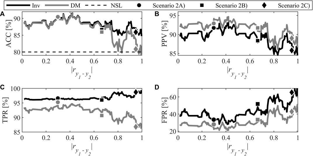
FIGURE 5. Classification performance for Scenario 2: (A) Accuracy, (B) Positive Predictive Value, (C) True Positive Rate, and (D) False Positive Rate. The symbols mark the specific combinations investigated further, and their color indicate the method (DM or inversion).

First, the accuracy is analyzed as it gives an overview of classification performance since it measures the proportion of well-classified samples. Classification performance is judged against the so-called no-skill line (NSL). The latter represents the accuracy that would be obtained if the samples were randomly assigned to a class. The performance of a useful classifier needs to be above the NSL. As the ratio of good to bad samples is 4:1 in this study, the NSL is set at 80%. Except for a few regions obtained from direct mapping with combination of highly-correlated quality attributes, the accuracy is above the no-skill line. This shows that both methods performed better than making random decisions. Also, for low to moderate levels of correlation (i.e., up to 60%) accuracy is almost the same for both methods. To discriminate both methods in this zone, other metrics need to be analyzed.

It is possible to observe that a distinction exists between both methods at all correlation levels. The PPV is greater for direct mapping which means the classifier has a better precision. However, the TPR rate is lower because the predictions for the positive class is better with the inversion. Usually, a compromise between TPR and PPV needs to be achieved to identify the best classifier. Also, it can be observed that the FPR is lower for direct mapping. This is considered an advantage for DM when the goal is to minimize the risk of producing bad quality products, since the probability of accepting a bad lot is lower.

For levels of correlation higher than 60%, the gap between the two methods widens especially for the TPR metric. The DM technique becomes more restrictive and generate more rejection of good lots of raw materials whereas the region obtained with inversion leads to accepting all the good lot as it tends toward 100%. For the FPR, a large increase is observed for both methods. However, even if the rate doubles and seems more drastic compared to the other metrics, it is normal to have higher values since there are fewer bad lots than good ones. Based on the ratio of bad and good samples, an increase of one FP leads to an increase of 4% of the FPR, while an increase of one FN causes a decrease of 1% of the TPR.

To better understand what happens when the level of correlation increases, three examples were drawn from the set of 148 combinations to compare the acceptance regions obtained with both techniques as collinearity between quality attributes increase. The simulator’s parameters used for these examples and their respective level of correlation is presented in Table 2 (Scenarios 2A–C). The classification metrics for all three examples are shown in Figure 5 using markers. The marker shape discriminates the level of collinearity, and its color is associated with the methods (DM or inversion).

As shown in Figure 6A, at low levels of correlation (here 30%), the two regions are almost the same. This explains why the accuracy was quite identical for DM and inversion. When collinearity increases to 66% (Figure 6B), a slight difference between the regions is observed. The largest region obtained by inversion increases acceptance of good lots at the expense of bad lots. The same observation can be made from Figure 6C when the correlation level is very high, i.e., 95%.

FIGURE 6

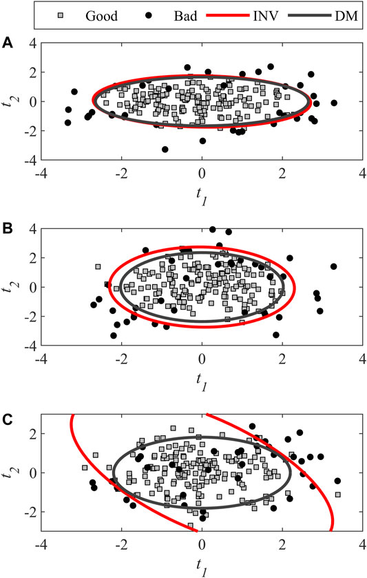
FIGURE 6. Score plot showing the specification regions obtained with DM and inversion for different levels of correlation between the quality attributes (Scenario 2): (A) 30%, (B) 66%, and (C) 95%.

The three examples need to be compared together to explain the cause of increasing FPR with collinearity. As the level of correlation increases, good and bad products in the score space overlap to a greater extent which increases the difficulty to obtain distinct classes. This can also be observed in Table 2 through the compromise between type I and II errors used for choosing the $\eta$ constant in direct mapping. The percentage of classification errors increases with collinearity to achieve the desired balance between the two types of errors. This does not seem to be caused by the model performance in prediction since at high levels of correlation the model has a Q²Y value of 90% as shown in Table 2, which is the case at low levels of correlation. The most likely cause for this behavior is that bad lots projecting near the origin of the scores space (i.e., generating a FP) are associated with observations in the y-space located in close to the edge of the product acceptance limit, but near the origin.

A particular attention should be paid to changes in the trends of TPR for both methods at high levels of correlation, which differ from those of other metrics. For DM, the TPR decreases and this may be explained similarly as for the increase in FPR. As the overlapping of the two product classes in score space is more important, the specification region needs to be more restrictive for good lots which generates more FN to obtain the same performance in terms of type I and II errors.

For PLS inversion, however, the trend is very different. The TPR increases to 100%, which means accepting all good lots of raw materials. Scenario 2C) in Figure 6C illustrates this situation. The ellipse obtained by inversion is stretched over the latent space which results in an acceptance region that includes a larger area where there are no or very few points (i.e., there is a risk of model extrapolation). The reason behind this behavior originates from the inversion of the ${\mathbf{C}}^{\text{'}}$ matrix. When the correlation increases between the two y-variables, this is reflected in the y-loading matrix $\mathbf{C}$, which eventually becomes ill-conditioned. Inverting this loading matrix increases of the norm of the scores and results in a larger ellipse. This is just like what happens to ordinary least squares regression parameters when highly correlated predictors are used.

Globally, Scenario 2 allowed showing that high correlation levels between both y-variables (i.e., higher than 80%) influences the classification performance of both methods. This may be caused by the proximity of observations to the product quality attribute acceptance limit in the y-space, the increasing overlap between both product classes in score space and model extrapolation for inversion. Concerning the classification performance itself, a distinction between both methods is observed for all the metrics. Direct mapping obtains a better FPR at the expense of TPR compared to the inversion where the relationship is opposite. Which one is best depends on the specific context and the relative cost of FPR vs. TPR.

4.2.2 Scenario 3: Impact of Collinearity when A < K

The third scenario illustrates the inversion Case 2 in which the number of PLS components is smaller than the number of y-variables. As the model investigated further in this section has only one component, the multivariate specification region in the latent space boils down to univariate limits (i.e., lower and upper bounds). Applying PLS inversion to several points on the product acceptance ellipse results in scores evolving between a minimum and a maximum value. These are used to define the univariate limits.

The simulations used to generate data in this study only led to a few combinations where A < K, and in all of those cases, A = 1 (see Figure 4). The 18 occurrences generated concentrate in the high correlation levels (i.e., mostly above 0.9). The classification performance is presented in Figure 7. Compared to Figure 5, the classification metrics are noisier due to the fact that the moving average was not apply due to the low number of samples.

FIGURE 7

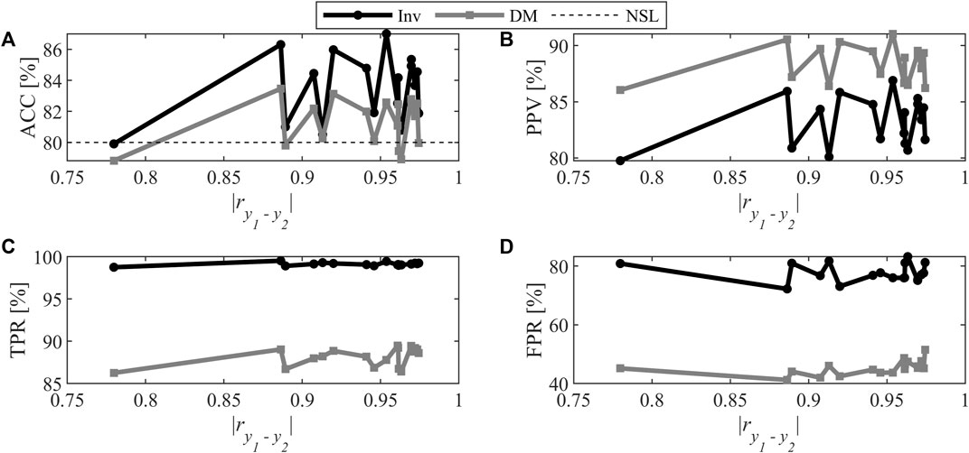
FIGURE 7. Classification performance for Scenario 3: (A) Accuracy, (B) Positive Predictive Value, (C) True Positive Rate, and (D) False Positive Rate.

Determining the impact of correlation is more difficult for this scenario since no information are available for the level of correlation ranging between 0 and 0.75. For the available data, a distinction between both methods can be observed in Figure 7 for each metric, and is comparable to Scenario 2. For the same range of correlation, the direct mapping provides similar performance for both scenarios. For the inversion, using one component leads to PPV and FPR that are slightly worse compared to what is obtained with two components. For the TPR, the same behavior is observed where the values tend toward 100%. This was expected since the inversion cases 1 and 2 are obtained by minimization of prediction errors (e.g., for case 1, the resulting objective function value is 0).

For the same range of levels of correlation, the conclusions drawn for Scenario 3 are similar to those of Scenario 2. However, if FPR in inversion had been chosen as the criteria to determine the number of components it might be expected that some of these samples would have been moved to Scenario 2 (A = K) since for the same range of correlation level, the FPR is lower when using A = K. This shows that the criteria used for determining the number of components influence the distribution of the sample between the three inversion cases.

4.2.3 Scenario 4: Impact of Collinearity When A > K

The last scenario considers the situations where A > K. In the context of this study, this means that three PLS components leads to the best accuracy in inversion. In contrast with Scenario 2, the specification regions obtained by inversion are not bounded due to the existence of a null space. For this reason, the specification regions were established in three ways and compared: inversion alone (NS), inversion constrained by the KS $\left(\text{NS}\cap \text{KS}\right)$, and DM. For the different levels of correlation, the performance of the methods is presented in Figure 8. As for Scenario 2, a moving average window was applied to remove noise and make the interpretation clearer.

FIGURE 8

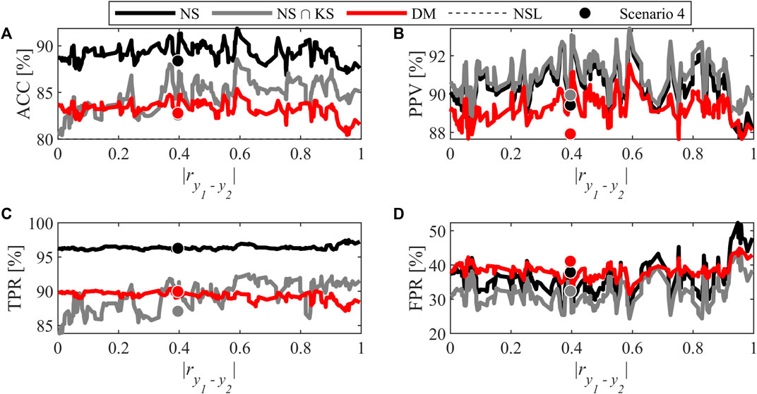
FIGURE 8. Classification performance for Scenario 4: (A) Accuracy, (B) Positive Predictive Value, (C) True Positive Rate, and (D) False Positive Rate. The symbols mark a specific combination investigated further, and their color is used to identify the method (DM or inversion).

For accuracy and TPR, a large gap exists in the inversion results when constraining the region to be within the KS or not. This makes sense since adding a limit on the knowledge space tightens the specification region, and makes it more restrictive. The chance of rejecting a good lot is increased, which leads to a reduced number of well-classified good lots. Considering these two metrics, when bounded, the inversion technique gives similar performance compared to the direct mapping.

However, for PPV and FPR, the performance of PLS inversion using both approaches are very similar. The KS bounding does not seem to have an impact or only a slight one on the misclassification of bad lots. The difference observed in ACC is then mainly caused by misclassification of good lots. By comparing the inversion and direct mapping, the PPV in Figure 8 shows that inversion is slightly better mainly because of lower FPR for this technique. However, the gap between the two techniques is smaller compared to Scenario 2. For the FPR in direct mapping for low to moderate correlation levels, adding one PLS component seems to double the rate when Figure 8 and Figure 5 are compared. This suggests that if the number of components had been selected using the FPR obtained by direct mapping, the partition of combinations might have been different. When testing this hypothesis, for almost all combinations, the number of components minimizing FPR is achieved using two components (i.e., A = K).

Figure 8 also allows interpreting the impact of the collinearity between the y-variables. Compared with Scenario 2, the correlation does not seem to have an impact on performance. Even when some fluctuations are present, the performance are relatively stable, and no systematic trend is observed in the different classification metrics. In addition, the performance at high levels of correlation does not degrade as observed in Scenario 2. In the latter, a unique solution exists for all combinations. For Scenario 4, the system of equations to solve is under-determined because the number of components (i.e. scores) is greater than the number of equations. The solution provided by Eq. 24 results from the minimization of the Euclidian norm of the score vector under the hard constraint imposed by Eq. 20. This forces the solution to be close to the origin of the latent space and results in a tighter and bounded specification region. The impact of collinearity between y-loading (i.e., c’s) seems less important, and the TPR tend to be more stable (i.e., no increase as for Scenario 2).

In addition, Scenario 4 allows showing that specifications in three dimensions are more difficult to use compared with Scenario 2. To illustrate the situation, an example named Scenario 4, is drawn from the different combinations of y-variables requiring three PLS components. Table 2 shows the parameters used to build the specification region while Figure 8 shows the performance metrics of the selected combination using a makers (dots). This example is representative of the average performance across all levels of correlation. Figure 9 shows the difference between inversion and DM in terms of the size of the specification regions. For ease of interpretation, the direct mapping and inversion are presented in different plots but using the same scale.

FIGURE 9

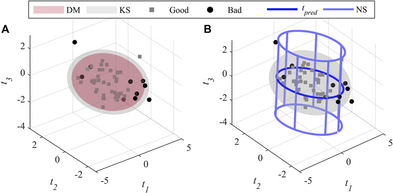
FIGURE 9. Example of an acceptance region for the case A > K using a 3 components PLS model obtained by (A) direct mapping, and (B) inversion.

As in Scenario 2, the DM technique shown in Figure 9A) leads to a smaller region included in the knowledge space compared to inversion. Figure 9B) presents the predicted score vector ${\mathit{t}}_{\mathit{p}\mathit{r}\mathit{e}\mathit{d}}$, the one that minimises the distance to the origin of the latent space for all the combination of y-variables. The null space representation is shown using a light color to provide a clearer image. In fact, the real representation is an elliptical cylinder where the periphery is modelled by an infinity of NS lines. If the region is unbounded, the new prediction needs to fall within the cylinder. When bounded, the point should fall at the intersection of the KS ellipsoid and the cylinder to be classified as a good lot. Thus, it is necessary to test the limit of the Hotelling T² first, and then to determine if the observation falls within the cylinder. Since the equation representing the specification region is unknown, it is more difficult to assess the position of a new observation using an automatic approach compared to DM.

4.3 Advantages and Drawbacks of the Methods

The various scenarios investigated allowed to identify the main advantages, and drawbacks of the two methods used for defining multivariate specification regions. This section wraps-up all the observations made through previous analyses and highlights the most important points to consider when choosing the method used to define the regions in Table 3.

TABLE 3

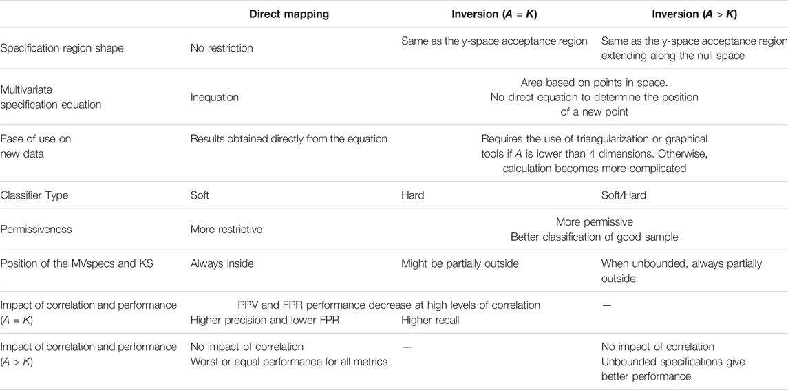
TABLE 3. Summary of the main features of direct mapping and inversion techniques.

Globally, the direct mapping approach is more restrictive in terms of volume/area compared with the inversion as the selected region is always included within the knowledge space. This can also be seen as an advantage since the user does not need to define a second limit to be within the KS. Furthermore, the DM allows a higher level of flexibility regarding the choice of the specification region shape. The inversion technique forces a similar shape to the product acceptance region in the y-space.

The type of classifier resulting from both approaches is different. Direct mapping provides a soft classifier since a choice is made by the user to set the limit. The limits can be adjusted by using the most relevant or important classification metric based on the specific objective of the case considered, for example to minimize acceptance of bad lots (i.e., FP). On the other hand, with inversion, no degree of freedom is available to adjust the position of the region based on the classification performance. The only exception is when choosing the number of components to use in the model. However, if the region is restricted to lie within the KS, the classifier becomes soft since the user needs to specify the confidence level of the T² limit.

The previous results have shown that it is easier to calculate the performance in classification and the location of a new sample against the specification region with direct mapping since it involves solving a simple inequality. To calculate performance using inversion, the equation of the resulting region is difficult to obtain, at the least. For example, the elliptical cylinder shown in Figure 9 is constructed with a series of points. The current technique to determine whether a point falls within the specification region obtained by inversion requires performing triangularization of the area. This leads to more complex calculation compared to direct mapping where it is straightforward to use the ellipsoid equations to determine if a new prediction is included or not in the acceptance region. For 2-dimensional cases, an easier way would be to use a graphical tool to check where the point fall compared with the region. The same approach could be used for 3 dimensions, but it would be more difficult to determine if the predicted point is within the specification region volume. For more than 4 components, further research is needed to find the best way to calculate the positioning of a new lot automatically.

Based on these analyses, identifying the best approach for defining specification regions is not straightforward and depends on the user’s objective. As classification performance is not superior for all the metrics for either method, one of them cannot be discarded. A compromise needs to be made during the development stage. PLS model inversion should be used when the cost of false negatives (FN) is higher than that of false positives (FP), and maximizing recall (or TPR) should be prioritized, and/or when the user prefers defining the shape of the specification regions using the PLS model structure. Otherwise, the direct mapping approach should be considered. Also, a careful attention should be paid when the y-variable are very correlated. This may lead to degradation of the classification performance. As a solution, using fewer y-variables to reduce redundancy or performing PCA on the y-space and using the scores to define the specifications could provide simple alternatives (Jaeckle, 1998).

5 Conclusion

The variability of raw materials is increasing, and affects the quality of the final product in many industries. To mitigate the situation, efforts are made to improve quality control. A key solution is to establish specifications regions for the properties of incoming lots of raw materials to detect unsuitable materials before processing it. In this work, a comparative analysis of two data-driven approaches for establishing multivariate specification regions using PLS models is proposed, namely the direct mapping and PLS inversion. Their classification performance is compared using multiple metrics. A focus was made on assessing the impact of collinearity in the y-space on the region classification performance.

It was shown that classification performance of bad quality lots of raw materials are poorer when quality attributes are highly correlated, when the number of PLS components is less than or equal to the number of y-variables. At low to moderate levels of correlation, the performance is slightly better for direct mapping when minimizing the false positive rate (TPR) or, alternatively Type II errors, is prioritized (i.e., reducing the risk of accepting poor quality raw materials). For the case where the PLS model has more components than the number of quality attributes, the performance is quite stable across the range of correlation levels. Both methods give similar classification performance when the specification region obtained by inversion is included within the knowledge space.

This study has shown that the decision of choosing a method for defining multivariate specification regions for raw materials depends on different factors. None of the method is superior in all possible cases. Direct mapping offers a higher degree of flexibility in the definition of the multivariate specification compared to inversion since the user can choose the shape of the region, and adjust its size/volume based on the most relevant criteria for a given industrial application. This technique is also advantageous in terms of computing resources as it requires solving an inequality to determine whether a new observation falls inside the region or not instead of the more complex approaches required with inversion. All in all, the work presented should be considered as a guide for establishing multivariate specifications regions for incoming raw materials. Knowing the main advantages/drawbacks, and selecting the most relevant classification metric for their application will help users choosing the most appropriate approach for defining their specification regions.

Data Availability Statement

The raw data supporting the conclusion of this article will be made available by the authors, without undue reservation.

Author Contributions

AP led this research, performed the simulations, analysed the results and wrote the manuscript. CD and ÉP supervised the work, and reviewed the manuscript.

Conflict of Interest

The authors declare that the research was conducted in the absence of any commercial or financial relationships that could be construed as a potential conflict of interest.

Publisher’s Note

All claims expressed in this article are solely those of the authors and do not necessarily represent those of their affiliated organizations, or those of the publisher, the editors and the reviewers. Any product that may be evaluated in this article, or claim that may be made by its manufacturer, is not guaranteed or endorsed by the publisher.

Acknowledgments

The authors acknowledge financial support of the Natural Sciences and Engineering Research Council of Canada (NSERC) (RGPIN-2019-04800 and ESD3-547424-2020) and the Fonds de Recherche Nature et Technologie (FQRNT) (Scholarship 287725).

References

Amsbary, R. (2013). Raw Materials: Selection, Specifications, and Certificate of Analysis. Quality Assurance & Food Safety [Online]. Available at: https://www.qualityassurancemag.com/article/aib0613-raw-materials-requirements/ (Accessed June 20, 2021).

Google Scholar

Azari, K., Lauzon-Gauthier, J., Tessier, J., and Duchesne, C. (2015). Establishing Multivariate Specification Regions for Raw Materials Using SMB-PLS. IFAC-PapersOnLine 48 (8), 1132–1137. doi:10.1016/j.ifacol.2015.09.120

CrossRef Full Text | Google Scholar

Bano, G., Facco, P., Meneghetti, N., Bezzo, F., and Barolo, M. (2017). Uncertainty Back-Propagation in PLS Model Inversion for Design Space Determination in Pharmaceutical Product Development. Comput. Chem. Eng. 101, 110–124. doi:10.1016/j.compchemeng.2017.02.038

CrossRef Full Text | Google Scholar

De Smet, J. (1993). Development of Multivariate Specification Limits Using Partial Least Squares Regression. Master. Hamilton, ON, Canada: McMaster University.

Google Scholar

Duchesne, C., and MacGregor, J. F. (2004). Establishing Multivariate Specification Regions for Incoming Materials. J. Qual. Technol. 36 (1), 78–94. doi:10.1080/00224065.2004.11980253

CrossRef Full Text | Google Scholar

Facco, P., Dal Pastro, F., Meneghetti, N., Bezzo, F., and Barolo, M. (2015). Bracketing the Design Space within the Knowledge Space in Pharmaceutical Product Development. Ind. Eng. Chem. Res. 54 (18), 5128–5138. doi:10.1021/acs.iecr.5b00863

CrossRef Full Text | Google Scholar

García-Muñoz, S., Dolph, S., and Ward, H. W. (2010). Handling Uncertainty in the Establishment of a Design Space for the Manufacture of a Pharmaceutical Product. Comput. Chem. Eng. 34 (7), 1098–1107. doi:10.1016/j.compchemeng.2010.02.027

CrossRef Full Text | Google Scholar

García-Muñoz, S. (2009). Establishing Multivariate Specifications for Incoming Materials Using Data from Multiple Scales. Chemometrics Intell. Lab. Syst. 98 (1), 51–57. doi:10.1016/j.chemolab.2009.04.008

CrossRef Full Text | Google Scholar

Godoy, J. L., Marchetti, J. L., and Vega, J. R. (2017). An Integral Approach to Inferential Quality Control with Self-Validating Soft-Sensors. J. Process Control. 50, 56–65. doi:10.1016/j.jprocont.2016.12.001

CrossRef Full Text | Google Scholar

Haibo He, H., and Garcia, E. A. (2009). Learning from Imbalanced Data. IEEE Trans. Knowl. Data Eng. 21 (9), 1263–1284. doi:10.1109/TKDE.2008.239

CrossRef Full Text | Google Scholar

ICH (2009). “Pharmaceutical Development Q8(R2). ICH Harmonised Tripatite Guideline [Online]. Available at: https://database.ich.org/sites/default/files/Q8%28R2%29%20Guideline.pdf (Accessed June 20, 2021).

Google Scholar

Jackson, J., and Edward, A. (1991). User’s Guide to Principal Components. New York: John Willey Sons. Inc., 40.

Google Scholar

Jaeckle, C. M., and MacGregor, J. F. (1998). Product Design through Multivariate Statistical Analysis of Process Data. Aiche J. 44 (5), 1105–1118. doi:10.1002/aic.690440509

CrossRef Full Text | Google Scholar

Jaeckle, C. M., and MacGregor, J. F. (2000). Industrial Applications of Product Design through the Inversion of Latent Variable Models. Chemom. Intell. Lab. Syst. 50, 199–210. doi:10.1016/S0169-7439(99)00058-1

CrossRef Full Text | Google Scholar

Jaeckle, C. M. (1998). Product and Process Improvement Using Latent Variable Methods. PhD. Hamilton, ON, Canada: McMaster University.

Google Scholar

MacGregor, J. F., and Bruwer, M.-J. (2008). A Framework for the Development of Design and Control Spaces. J. Pharm. Innov. 3 (1), 15–22. doi:10.1007/s12247-008-9023-5

CrossRef Full Text | Google Scholar

MacGregor, J. F., Liu, Z., Bruwer, M.-J., Polsky, B., and Visscher, G. (2016). Setting Simultaneous Specifications on Multiple Raw Materials to Ensure Product Quality and Minimize Risk. Chemom. Intell. Lab. Syst. 157, 96–103. doi:10.1016/j.chemolab.2016.06.021

CrossRef Full Text | Google Scholar

Nomikos, P., and MacGregor, J. F. (1995). Multivariate SPC Charts for Monitoring Batch Processes. Technometrics 37 (1), 41–59. doi:10.1080/00401706.1995.10485888

CrossRef Full Text | Google Scholar

Palací-López, D., Facco, P., Barolo, M., and Ferrer, A. (2019). New Tools for the Design and Manufacturing of New Products Based on Latent Variable Model Inversion. Chemom. Intell. Lab. Syst. 194, 103848. doi:10.1016/j.chemolab.2019.103848

CrossRef Full Text | Google Scholar

Tessier, J., and Tarcy, G. P. (2010). Multivariate Specifications of Raw Materials: Application to Aluminum Reduction Cells. IFAC Proc. Vol. 43 (9), 1–6. doi:10.3182/20100802-3-ZA-2014.00001

CrossRef Full Text | Google Scholar

Tomba, E., Barolo, M., and García-Muñoz, S. (2012). General Framework for Latent Variable Model Inversion for the Design and Manufacturing of New Products. Ind. Eng. Chem. Res. 51 (39), 12886–12900. doi:10.1021/ie301214c

CrossRef Full Text | Google Scholar

Weiss, G. M. (2013). “Foundations of Imbalanced Learning,” in Imbalanced Learning. Editors H. He, and Y. Ma (Piscataway, NJ: IEEE Press).

CrossRef Full Text | Google Scholar

Wierda, S. J. (1994). Multivariate Statistical Process Control-Recent Results and Directions for Future Research. Stat. Neerland 48 (2), 147–168. doi:10.1111/j.1467-9574.1994.tb01439.x

CrossRef Full Text | Google Scholar

Wold, S., Sjöström, M., and Eriksson, L. (2001). PLS-Regression: a Basic Tool of Chemometrics. Chemom. Intell. Lab. Syst. 58 (2), 109–130. doi:10.1016/S0169-7439(01)00155-1

CrossRef Full Text | Google Scholar

Yu, L. X., Amidon, G., Khan, M. A., Hoag, S. W., Polli, J., Raju, G. K., et al. (2014). Understanding Pharmaceutical Quality by Design. Aaps J. 16 (4), 771–783. doi:10.1208/s12248-014-9598-3

PubMed Abstract | CrossRef Full Text | Google Scholar