Synchronization-Free Multivariate Statistical Process Control for Online Monitoring of Batch Process Evolution

Introduction

Industrial sectors often rely on batch processes to produce their intermediate or final products. Batch processes consist of cyclic repetitions of an established recipe aiming at the production of products meeting specific quality specifications. They are also characterized by complex, dynamic and nonstationary behavior. Thus, monitoring a batch evolution in real-time is a challenging, but essential action to obtain end products with desired quality, reducing costs and increasing process understanding. (van Sprang et al., 2002; Rendall et al., 2019; Rato and Reis, 2020).

Nowadays, with the emergence of Industry 4.0, batch processes are monitored not only with typical process sensors, e.g., temperature, pressure, flow, etc, but also with advanced sensors probes based on spectroscopic techniques such as near-infrared (NIR), mid-infrared, and Raman (Cimander and Mandenius, 2004; Pöllänen et al., 2006; Ávila et al., 2012; Besenhard et al., 2018; Grassi et al., 2019; Avila et al., 2021). The collection and use of process sensor measurements from historical batches that followed the normal operating conditions (NOC) and reached the targeted product specifications is the basis for the development of multivariate statistical process control (MSPC) models and related charts, ready to be used to test the evolution of new batches (Kourti, 2005; Ferrer-Riquelme, 2009; Wold et al., 2009; Colucci et al., 2019; Vidal-Puig et al., 2019; França et al., 2021). Offline MSPC charts can be used to diagnose the root cause of a disturbance from a finished faulty batch. However, it is even more important the online use of MSPC charts for real-time monitoring of batch evolution to enable taking quick action in case of detection of process disturbances.

Process data measurements from a single batch consist of the collection of several variables, $J$, (process data and/or spectroscopic measurements) at different process points throughout the batch, $K_i$. These measurements are usually organized in a data matrix, ${\mathbf{X}}_{\mathbf{i}}$, with dimension $(K_i\times J)$ to be used for process monitoring and/or control purposes. Most data-driven modeling strategies aiming at building online MSPC charts to monitor process evolution require that data from several NOC batches, $I$, that have the same batch length, i.e. batch data matrices with the same numbers of rows $K, \text{and}$ follow the same and synchronized process dynamics. When this happens, the data can be arranged in a three-dimensional data array, $\underset{¯}{\mathbf{X}}$, with dimensions $I\times K\times J$. Most of the MSPC models are built based on data-driven multivariate analysis methods, such as principal component analysis (PCA) and partial least squares (PLS); for this purpose, different unfolding strategies of the $\underset{¯}{\mathbf{X}}$ array can be used according to the modeling approach used as originally introduced elsewhere (Nomikos and MacGregor, 1995; Wold et al., 1998). However, because of the inherent batch process complexity and nonstationary behavior, the batch duration, $K_i$, is not always the same and equally relevant, key process events do not occur at the same time point when comparing different NOC batch runs of the same process. This uneven and not synchronized batch data cannot be represented in this perfect three-dimensional data array, $\underset{¯}{\mathit{X}}$, unless adjusted using different batch synchronization tools to cope with this problem (González-Martínez et al., 2014b).

Great progress has been made to develop strategies for batch alignment based on a maturity index or indicator variable coming directly from a process variable or estimated by PLS models or using more advanced algorithms, such as correlation optimized warping or dynamic time warping (Kassidas et al., 1998; Ramaker et al., 2004; González-Martínez et al., 2014a; Liu et al., 2017; Spooner and Kulahci, 2018; Zhao et al., 2020). Most of these methods were designed for the monitoring of finished batches using offline MSPC models and only an attempt proposed by (González-Martínez et al., 2011) described a method based on time warping that allows batch alignment for online MSPC.

Despite the methodologies mentioned above, having naturally non-synchronized batches is the most common situation in practice and batch alignment is a delicate operation that can induce artifacts in the definition of MSPC models when scarce information is available or when is not properly applied. Hence, the need for MSPC approaches that can circumvent the synchronization step for online process monitoring and control. Very few attempts have been carried out in this direction. (Rato et al., 2017) used the translation-invariant wavelet decomposition and PCA for the monitoring of the semiconductor manufacturing process. Another method based on a search grid capturing the batch trajectory in the PCA score space was proposed by (Westad et al., 2015) and was used for the monitoring of two industrial processes.

In this paper, a new synchronization-free approach of multivariate statistical process control (MSPC) for online monitoring and diagnostics of batch processes is introduced. It is based on the modeling of an overall NOC historical batch trajectory, defined by individual non-synchronized NOC batches, and the subsequent construction of derived PCA-based local MSPC models covering the complete process, i.e., the complete overall NOC batch trajectory. These local models are used to identify whether new batch observations are inside the NOC trajectory and, when this is the case, to provide an estimate of the process progress. The approach is illustrated using two real examples of NIR-monitored batch processes but is readily applicable for the online monitoring of batch processes of different typologies monitored by one or more diverse sensors.

Process Case Studies and Data Sets

Two case studies from previous works are used to illustrate and test the online batch MSPC models for tracking process trajectories. A brief experimental description of these NIR-monitored processes with the related spectral preprocessing implemented is presented below.

Process 1: Fluidized Bed Drying of Pharmaceutical Granules

Batches of 500-g pharmaceutical wet granules (dry mass fraction of mannitol > 50% and excipients) were dried in a 4-L fluidized bed (4M8-Trix Formatrix, ProCepT, Belgium). The fluidized bed air inlet flow was controlled at 0.6 or 0.85 m³/min and a temperature range from 22 to 30°C. In-line NIR measurements were collected approximately every second using a spectrophotometer with a MEMS Fabry-Perot interferometer (N-Series 2.2, Spectral Engines, Finland) coupled to a diffuse reflectance immersion probe (OFS-6S- 100HO/080704/1, Solvias, Switzerland). The spectra covered a wavelength range from 1750 to 2150 nm at 1-nm intervals. For each batch, off-line reference moisture content analysis was carried out using a thermogravimetric moisture analyzer (MB120, Ohaus, Germany) from samples retrieved at 6-min intervals to detect drying endpoint (moisture < 2%). Because of different process conditions at the beginning and during each batch run, such as inlet air temperature and flow, different batch durations were required for each trial to reach the defined <2% moisture level, therefore, providing data matrices with uneven lengths. Faulty batches used in the testing of the proposed approach did not reach this moisture level. Suitable preprocessing was employed to filter out noise and baseline fluctuations on the NIR raw data observations before data analysis. The preprocessing steps included the application of a moving average of consecutive NIR observations followed by standard normal variate (SNV) normalization. For a detailed description of the experimental procedure and the visualization of the spectral data, the reader is referred to (Avila et al., 2020; de Oliveira et al., 2020). Some batches were selected from the previous work and additional faulty batches were used for model validation. Ten NOC batches, NOC1 to NOC10, were used for MSPC model building, and three for validation (one NOC, Batch NOC1, and two faulty batches, Batch Fault1 and Batch Fault2). This is an example of a batch process where the evolution of drying in time is not synchronized among batches since the initial and final material in every batch does not necessarily have the same moisture level.

Process 2: Automated Benchtop Batch Gasoline Distillation

Batches of 100-ml gasoline blends (mixture of pure gasoline and ethanol) were distilled in an automated batch distillation device designed for the in-line monitoring of distilled product with NIR spectroscopy. For every batch, vapor temperature readings and in-line NIR absorption spectra (900–2600 nm with 4 cm⁻¹ resolution; Rocket, ARCoptix ANIR, Switzerland) were recorded for every unit of percentage distilled mass fraction of initial sample weight, in the 5–90% range. Therefore, the data matrices obtained had the same number of NIR observations per batch (86 NIR spectra) and every observation was related to the same distillation process stage, as defined by the percentage (w/w) of distilled sample mass. The gasoline batches were prepared by mixing ethanol AR (99% Sigma-Aldrich) and pure gasoline (from Petrobras refinery, Brazil) at different volume ratios from 10 to 40%. Distillation batches of gasoline blends with 27% ethanol were defined as NOC batches and all batches with a different ratio as faulty, or out of specification according to Brazilian legislation. The preprocessing steps used in this data set were Savitzky-Golay derivative (1^st-order derivative, 2^nd-order polynomial function and 9-point window) for baseline correction followed by spectral normalization to mitigate signal intensity fluctuations of the NIR spectra. More detailed information related to the experiments and spectra preprocessing can be found elsewhere (de Oliveira et al., 2017). In this work, nine NOC distillation batches were used to build the MSPC control charts for tracking process trajectory (B1 to B3, B5 to B9 and B11), and three for validation, where one was NOC (B4) and two were faulty batches (B13, B19). In this case, batch process trajectories were synchronized because the percentage of distillation weight gives a direct reference for batch progress evolution.

Data Treatment

The online batch MSPC model building procedure for tracking process evolution in synchronized or non-synchronized batch processes is described below. The complete methodology involves the following steps:

a) Modeling of NOC batch process trajectories.

b) Construction of local MSPC models based on NOC batch process trajectories.

c) Use of an MSPC chart based on local MSPC models to track the evolution of new batches.

The first two steps are involved in the generation of the MSPC models, whereas the last step involves the use of the local MSPC models on new batches to test whether they follow the NOC trajectory or to detect faults. A detailed description of each step is presented below together with a visual description of the approach in Figure 1.

FIGURE 1

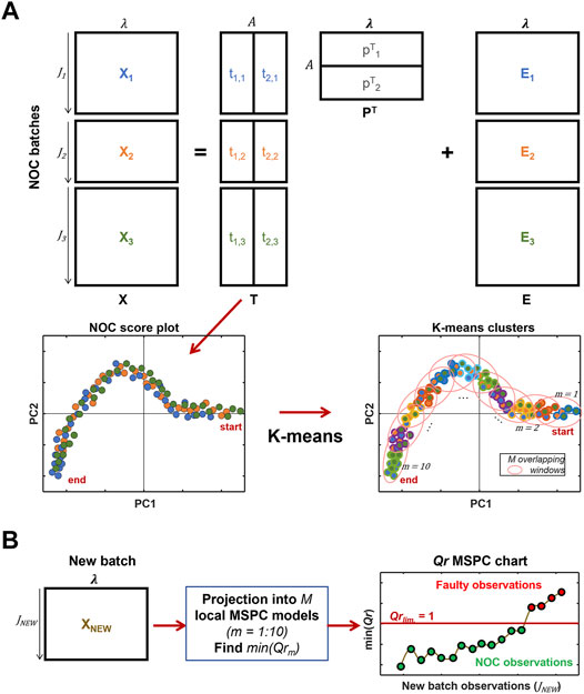
FIGURE 1. Illustrative description of the different steps involved in the implementation of the local MSPC models for online monitoring of batch evolution. (A) PCA modeling of original batch process data for several NOC batches, visualization of process trajectories in the scatter score plot and definition of local regions in the NOC trajectory using k-means. (B) Monitoring of the evolution of a new batch using the projection of each observation onto the local MSPC models. The related reduced Q-statistics control chart is obtained plotting the minimum Qr value obtained in all M model projections per each observation.

Modeling of NOC Batch Process Trajectories

The evolution of NOC batches, a.k.a “golden batches”, can be defined using different multivariate analysis modeling strategies, such as PCA, independent component analysis, multivariate curve resolution, parallel factor analysis, etc. (Haack et al., 2004; Mortensen and Bro, 2006; Skibsted et al., 2006; Bogomolov, 2011; de Oliveira et al., 2017; Gomes et al., 2019). In this work, we use PCA as the basis to define the general NOC batch process trajectory.

The NIR spectra obtained in a NOC batch i are structured in a data matrix ${\mathbf{X}}_{\text{i}}(K_i\times J)$, where $K_i$ are the number of spectra collected (related to time points for Process 1 and to % of distillation for Process 2) and $J$ are the NIR channels per spectrum.

When several NOC batches are used to define the general process trajectory, the data matrices from the different NOC batches, ${\mathbf{X}}_{\text{i}}(K_i\times J)$, are placed one on top of each other to build an augmented multiset structure $\mathbf{X}(N\times J)$, where $N$ is the number of rows related to the total number of observations from the $I$ NOC batches, that is, $N= {\displaystyle \sum }_i^I{K}_i$. Note that this strategy does not require resizing or synchronization of uneven batch lengths, since the only requirement is that all batches share a common spectral dimension, $J$ (Wold et al., 1998). The next step is to column mean-center this multi-batch structure and analyze it with PCA. This centering operation is not oriented to remove the mean trajectory of the batches in time, just to center the data and remove the average spectral shape in order to see the spectral process variation already from the first PC.

Principal component analysis (PCA) is used to obtain a global model of batch trajectories explaining the overall NOC process evolution. PCA is used to reduce the dimensionality of the preprocessed spectral data into a low-dimensional subspace of principal components (PC’s), orthogonal among them, that preserve the relevant information of the original data and explain the maximum non-random variance (Jolliffe, 2002). The PCA model for the augmented process data matrix $\mathbf{X}(N\times J)$ is expressed as in Eq. 1,

$\mathbf{X }= \mathbf{T}{\mathbf{P}}^{\mathbf{T}}+\mathbf{E}(1)$

where $\mathbf{T}(N\times A)$ is formed by the scores matrix, related to the observations of the batch process data, ${\mathbf{P}}^{\mathbf{T}}(A\times J)$ is the loadings matrix, related to the importance of the NIR variables in the description of the $A$ PC’s and $\mathbf{E}(N\times J)$ is the residual matrix after modeling. The number of principal components of the model, $A$, can be found using a suitable cross-validation method. The loading matrix, P^T, is common to all batches and the augmented score matrix, T, accommodates T_i blocks, related to every batch, that can be formed by a different number of observations, $K_i$. The multiset structure for three NOC batches and the related PCA model is illustrated in Figure 1A (top left), where λ represents the $J$ spectral channels of the NIR spectra.

Construction of Local MSPC Models Based on NOC Batch Process Trajectories

From the augmented score matrix of all NOC batches, individual batch score trajectories can be overlapped on a scatter score plot, as shown in Figure 1A (bottom left). The dots represent the scores for each observation and are colored according to the NOC batches used in the PCA model. Note that the overall trajectory evolution is the same for all NOC batches, but in a general non-synchronized case, the starting and endpoint of every batch do not need to coincide. The overlapped individual batch process trajectories define a global description of the variability of the NOC process evolution, helpful to observe whether a new batch process evolves as NOC batches or not, independently from the batch length and dynamics.

The evolution described by the overlapped NOC trajectories can be divided into a sufficient number of $C$ local regions using a cluster analysis methodology, such as k-means and fuzzy c-means clustering algorithms. In general, any algorithm allowing an even distribution of observations in the different clusters would be potentially valid in this step. The number of clusters used to set the local MSPC models will be closely related to the process progress resolution desired to study the batch evolution and will be limited by the number of available NOC observations. Hence, the higher the number of clusters, the higher process progress resolution will be obtained; however, care must be taken to avoid building local MSPC models with an insufficient number of observations that could lead to a non-representative description of the process stage to be controlled. Figure 1A (bottom right) illustrates these local regions for $C=11$, as indicated by the outer circle color of the neighbor observations inside each cluster. The seeding information for the local MSPC models is formed by the observations in two consecutive clusters. Therefore, the first local MSPC model contains the observations in the first two clusters of the process trajectory, the second local MSPC model uses the observations in clusters two and three and so forth until all the NOC process trajectory is covered. The observations used in consecutive local MSPC models overlap with each other so that all process trajectory regions are covered. As can be seen in Figure 1A, for a k-means analysis providing 11 clusters, 10 local MSPC models with overlapping information as defined by the red ellipses can be built.

The local MSPC models are built based on PCA and control chart limits are defined using the suitable local model statistics. The operational procedure to build each local MSPC model can be described as follows. First, the original observations, i.e. NIR spectra, for each local model are placed into a data matrix ${\mathbf{X}}_{\mathit{m}}(K_m\times J)$, where $m$ indicates the index of the local model (from 1 to M) and $K_m$ is the number of observations used to build the model. Then, this matrix is mean-centered and modeled with PCA, as in Eq. 1, generating the matrices of scores ${\mathbf{T}}_{\mathit{m}}(K_m\times {\text{A}}_{\text{m}})$, loadings ${\mathbf{P}}_{\mathit{m}}^{\mathbf{T}}(A_m\times J)$, and residuals ${\mathbf{E}}_{\mathit{m}}(K_m\times J)$. Note that the mean-center is performed using the mean of the matrix ${\mathbf{X}}_{\mathit{m}}$ not the global mean of the multi-bach structure. By doing so, since the local observations inside the matrix ${\mathbf{X}}_{\mathit{m}}$ should have similar spectral shape, the mean trajectory of the batch at that particular process stage is removed. Enough PC’s, $A_{\text{m}}$, are included in each local model to provide the best fit using cross-validation (Wold, 1978). Finally, the control limits of the local control charts can be derived using the residuals and the scores from the local PCA model (Rännar et al., 1998; Wold et al., 1998; Aguado et al., 2007). In this work, the controls charts are based only on the residual matrix, ${\mathbf{E}}_{\mathit{m}}$, deriving the Q-statistic control chart limit, $Q_{lim}$; however, other statistical parameters can readily be used to track the process evolution. The $Q_{lim}$ is calculated according to the equation proposed by (Jackson and Mudholkar, 1979). Thus, once the local MSPC models and their related multivariate control charts limits are set, the online process evolution of new batches can be tracked based on the local models defined.

Use of an MSPC Chart Based on Local MSPC Models to Track New Batch Evolution

Calculation of squared residuals statistics (Q)

For online batch monitoring of new batch observations (${\mathbf{X}}_{\mathbf{NEW}}$ in Figure 1B), every new observation is projected onto all local MSPC models and a set of the related sum of squared residuals statistics, , are obtained as shown in Figure 1B. Thus, for every new online observation, ${\mathbf{x}}_{\text{k}}$ (a NIR spectrum in X_NEW), its scores values, ${\mathbf{t}}_{\text{k},\text{m}}$, are obtained for each local MSPC model using its related PCA loadings, ${\mathbf{P}}_{\mathrm{m}}$, as follows,

${\mathbf{t}}_{\text{k},\text{m}} = {\mathbf{x}}_{\text{k}}{\mathbf{P}}_{\text{m}}(2)$

Then, the residuals for the new observation in each local model are obtained as,

${\mathbf{e}}_{\text{k},\text{m}} = {\mathbf{x}}_{\text{k}}-{\mathbf{t}}_{\text{k},\text{m}}{\mathbf{P}}_{\text{m}}^{\text{T}}(3)$

And the related $Q_{k,m}$ as:

$Q_{k,m}={\mathbf{e}}_{\text{k},\text{m}}{\mathbf{e}}_{\text{k},\text{m}}^{\mathbf{T}}(4)$

For an easier interpretation of the global multivariate control chart obtained from the outputs of the local MSPC models, reduced Q-statistics, $Q{r}_{k,m}$, are calculated by dividing the obtained $Q_{k,m}$ values by the related local model $Q_{lim}$. Thus, the control limits for all local MSPC models become equal to one, $Q{r}_{lim}=1$. The reduced Q values for every new observation, $Q{r}_{k,m}$, are checked to see whether they are above or below the $Q{r}_{lim}$. If all $Q{r}_{k,m}$ values for the observation $k$ are large and above one, this observation is diagnosed as faulty, and it is an indicator that the process is deviating from the NOC trajectory. Conversely, if one or more $Q{r}_{k,m}$ values are below the control limit, the observation follows the NOC trajectory. An easy way to visualize the diagnostic of every new observation by using a single Q chart is shown in Figure 1B (bottom right), where only the minimum $Qr$ parameter after the projection in all local models is displayed for every new observation. Observations that follow the NOC trajectory are depicted by the green dots below the $Q{r}_{lim}=1$, and the eventual deviations from it, with $\text{min}\left(Q{r}_{k,m}\right)>1$, in red. To assess the spectral variables making the greatest contributions to the deviation in $Q$ we can display the Q-statistics contribution plots for the sought observation by plotting the elements of the residual vector, ${\mathit{e}}_{\mathit{k},\mathit{m}}$. The residuals used for the contribution plots are calculated using the best local MSPC model related to the last NOC observation.

For NOC observations, it is also possible to estimate the process stage of every observation by identifying the local MSPC model providing the lowest $Q{r}_{k,m}$ value. This visualization approach will be provided for the real process applications studied in this work in the next section.

Results and Discussion

In this section, the results related to the construction of NOC trajectories and local MSPC models for each process case study are shown. Afterwards, the resulting MSPC charts for the online monitoring of new NOC and faulty batches are shown for each process. Complementary visualization of MSPC charts and fault diagnostics based on contribution plots are also presented.

Construction of NOC Trajectories and Local MSPC Models

The construction of PCA-based NOC trajectories for each process was calculated as explained in step a of the Data Treatment section using the training dataset, i.e. all NIR observations from selected complete NOC batches. This step was followed by k-means analysis on the overlapped individual NOC batch trajectories to define the clusters used to build the local MSPC models covering the overall NOC process trajectory (Data Treatment section step b). Figure 2 shows the PCA score scatter plot and the k-means clusters used to build the local MSPC models describing the overall NOC batch process trajectories for the drying (Process 1) and the distillation processes (Process 2).

FIGURE 2

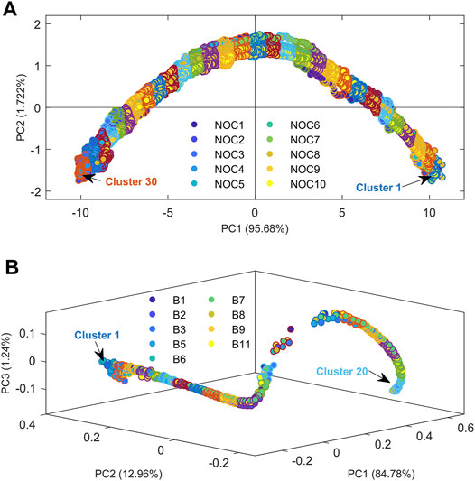
FIGURE 2. PCA score plot for the online NIR observations showing the NOC batch process trajectories and local clusters found by k-means for (A) Process 1, fluidized bed drying, and (B) Process 2, gasoline blend distillation. The inner part of the circles is colored according to the related NOC batch, whereas the outer part reflects the observations included in every cluster and, hence, in the related local MSPC model.

Principal Component Analysis of the NOC batches from Process 1 (Fluidized bed drying) allowed description of the process evolution using only two PC’s explaining a total of 97.61% of the data variance, as shown in the score plot of Figure 2A. The score plot described mostly the variation of the moisture content with the drying evolution from beginning to end of every NOC batch. Note that, because each batch had different initial and final moisture conditions, they started and finished at different points of the overall NOC trajectory; however, all individual batch trajectories followed the same evolution pattern, as shown in the PCA score plot. Once the overall NOC trajectory was defined, 30 clusters were defined using the k-means analysis along this trajectory, as displayed by the different outer circle colors associated with the observations inside each cluster in Figure 2A. For this example, 30 clusters and, hence, 29 local MSPC models, were considered sufficient to track in detail the process evolution. After that, a number indicating the process stage evolution was automatically assigned to each cluster according to the position in the overall NOC trajectory.

For Process 2 (Distillation), three components were required by PCA to explain 98.99% of NOC batches variance because of the complex gasoline sample and the continuous variation of the distilled material composition. The complex overall NOC trajectory associated with the distillation process is shown in the 3 PC score scatter plot in Figure 2B. Despite the higher complexity of the overall NOC trajectory linked to the distillation process, all individual batches trajectories followed the same evolution pattern with good reproducibility. In contrast to the drying process, the NIR observations of the distillation process were acquired at specific percentages of distillation weight; therefore, the observations were naturally synchronized according to the process evolution. Note that all batches started and finished at the same point of the overall NOC batch trajectory in the score plot. The k-means algorithm applied on the PCA scores of Figure 2B was used to set 20 clusters along the overall NOC batch trajectory, as displayed in Figure 2B. The number of clusters is lower than in the previous example because of the limited number of available observations per batch run (only 86) and the need to avoid having clusters with a very low number of observations to build the local MSPC models.

Once the overall NOC batch process trajectories were defined for each process case, the original NIR observations inside the suitable two consecutive k-means clusters were used as seeding information to build local MSPC models for each step of the batch trajectory, as described in the Data Treatment section (step b). Thus, a total of 29 and 19 local PCA-based MSPC models were built for Processes 1 and 2, respectively. Local MSPC control chart limits based on the Q-statistics with a 99% confidence interval were calculated for each local MSPC model to be used for the online tracking of new batches evolution, as shown in the next subsection.

Online Tracking of New Batch Evolution with Local MSPC Models

The results of the use of local MSPC models for the online tracking of new batch evolution are described separately for each process case, as shown below. The new batches used were identified in previous studies as NOC or faulty; therefore, they will be useful to demonstrate and validate the proposed methodology.

Application to Process 1 (Fluidized Bed Drying)

The tracking of every observation in new fluidized bed drying batches was performed as described in the Data treatment section (step c), using the 29 local MSPC models built as explained above (Supplementary Figure S1 and a related animation Supplementary Figure S2 of the help to display how the Qr values issued from every MSPC local model are obtained for every observation in a batch).

The Qr-based MSPC control charts for the online tracking of observations in two drying batches are shown in Figure 3. Figure 3A; Figure 3C are contour plots related to validation Batch NOC1 and Batch Fault1, respectively, that show all the Qr values calculated after the projection of each online NIR observation of the batch onto all local MSPC models. A log-scale colormap has been used to highlight the differences at low Qr values. The horizontal axis of the contour plot represents the batch time at which every observation was collected and the right vertical axis the indices related to the local MSPC model used to describe the Process 1 NOC batch trajectory, i.e. from 1 to 29. Additionally, in the left vertical axis, each local MSPC model index is associated with a percentage of the process progress from 0–100%, defined making a linear scaling that links the initial local model to 0% process progress and the final local model to 100% process progress. The process progress in this approach plays the same role as the process maturity concept proposed by other authors (Wold et al., 1998; Westad et al., 2015).

FIGURE 3

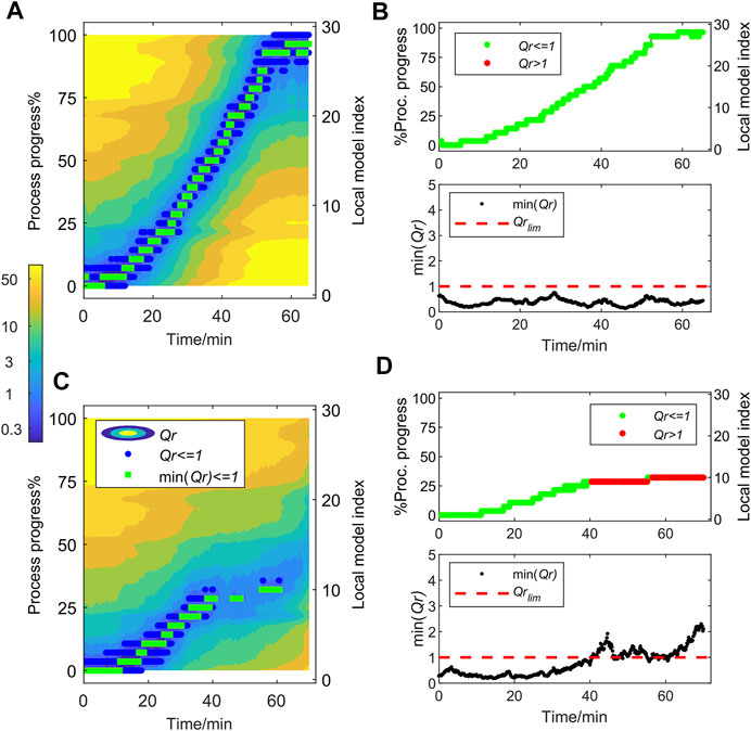
FIGURE 3. Qr-based MSPC charts for fluidized bed drying (Process 1) batch NOC1 (A and B) and batch Fault1(C and D). (A and C) Contour plots of the Qr values calculated after the projection of each NIR observation onto the local MSPC models. Blue dots show values of Qr < 1 (control limit), green squares the min (Qr < 1). (B and D) Charts show the min (Qr) value (bottom panel) and the related process progress associated with it (top panel) for every batch observation. In the process progress plot, NOC observations are displayed in green and faulty observations in red.

Thus, to track the behavior of an observation of a new batch, their related Qr values (associated with a specific process time) are examined. In the contour plots in Figure 3A; Figure 3C, the Qr values below the control limit, i.e. Qr < 1, are depicted as blue dots and the min (Qr < 1) for every observation in green. If an observation shows a NOC behavior (as all do in Figure 3A related to Batch NOC1), there will always be one or more Qr values below 1; i.e., all observations will show one or more blue dots and a green dot. Instead, when an observation deviates from the NOC trajectory, as in Batch Fault1 (Figure 3C), all Qr values related to that observation are above the control limit of 1 and neither blue nor green dots are observed.

To facilitate the interpretation and summarize the relevant information of the results in the contour plots, graphics displaying the min (Qr) value and the related process progress for every batch observation are proposed (see Figure 3B and Figure 3D for batches NOC1 and Fault1, respectively). Figure 3B shows that all observations for batch NOC1 followed the NOC batch trajectory, seen because all min (Qr) values were below the control limit of 1 (bottom panel) and that the process progress covered the complete range (0–100%) (top panel). Figure 3D shows that batch Fault1 deviated from the NOC trajectory after approximately 40 min of batch time as flagged by the Qr above the local MSPC control limits (min (Qr) > 1) (bottom plot). When a fault happens, the related observations are displayed in red in the process progress plot to indicate that the evolution of the process is abnormal (top plot).

Detailed results and interpretation of the abnormal behavior for the online tracking of two faulty batches, Fault1 and Fault2, are shown in the Supplementary Figure S3; Figure 4 (left plots), respectively. Supplementary Figure S3A; Figure 4A show the deviations of the two batches by displaying the score plot projections of NIR observations of these new batches onto the global PCA model used to describe the NOC batch trajectory. The score plot shows all training NOC batch trajectories as gray dots whereas the NOC observations from the new batches are overlayed as green dots when identified as NOC and as red dots when faulty. Supplementary Figures S3B, S3C; Figure 4B show the batch process progress and min (Qr) MSPC chart for the tracking of the online observations, where the abnormal observations are associated with min (Qr) values higher than 1 and flagged in red color in the process progress plot. Moreover, Q contribution plots from two faulty observations selected from each batch are shown in Supplementary Figure S3D; Figure 4C. The contribution plots were used to understand the reasons for the deviations from the NOC batch trajectory, as described below for each batch.

FIGURE 4

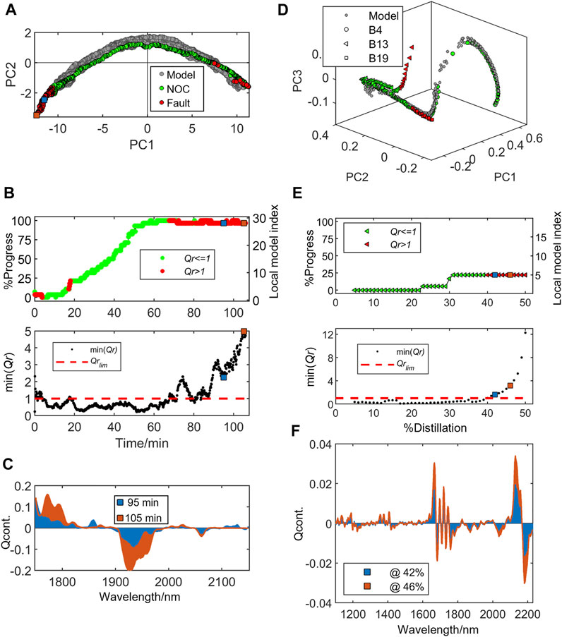
FIGURE 4. Online tracking of new batch evolution using the local MSPC models for process 1 (fluidized bed drying) left plots (A to C) and process2 (gasoline blend distillation) right plots (D to F). (A) Process 1 PCA score plot showing the training NOC batches trajectories (gray dots) and validation batch Fault2 trajectory in green (NOC observations) and red dots (faulty observations). (B) MSPC chart showing the process progress (top panel) and min (Qr)-based MSPC chart. (C) Q contribution (Qcont.) plots for two faulty observations at 95 and 105 min of batch Fault2 drying time represented by the blue and orange squares in the MSPC control chart. (D) Process 2 PCA score plot showing the training NOC batches trajectories (gray dots) and three validation batches (B4 circles, B13 triangles and B19 squares) trajectories in green (NOC observations) and red dots (faulty observations). (E) MSPC chart showing faulty batch B13 process progress (top panel) and min (Qr)-based MSPC chart. (F) Q contribution (Qcont.) plots for two faulty observations at 42 and 46% of distillation represented by the blue and orange squares in the MSPC control chart. Green and red marker face color in process progress chart indicate that the observation is inside or outside the trajectory confidence limits, respectively.

The deviation of drying batch Fault1 from the NOC trajectory was detected after approximately 40 min of batch time, see Supplementary Figures S3B, S3C. Although in Supplementary Figure S3A the faulty observations (red dots) right after 40 min were still close to the NOC trajectory, the related min (Qr) after projection onto local MSPC models was above the control limit indicating a deviation, which became even larger after ca. 65 min of batch time, see Supplementary Figure S3C. To help to diagnose this deviation, contribution plots are shown in Supplementary Figure S3D for two faulty observations selected at 64 and 69 min of batch time. These observations are marked in blue and orange squares in the score plot and MSPC charts. The Q contribution plots show that the absorption bands that gave higher contributions to Q were around 1750 and 1900 nm related to the 1^st overtone of CH and OH bonds. No clear trend was observed when comparing the contribution plots of the two observations suggesting that this deviation may have been caused by changes of heterogeneity or particle comminution of the pharmaceutical granules.

During the tracking of the additional batch, Fault2, three clusters of faulty observations were detected, see Figure 4B. The first faulty observations were detected during the first few minutes of the batch process. This deviation was related to the initial moisture content higher than the common starting point for the NOC batches used to build the MSPC models at the beginning of the process trajectory. However, after a few minutes of drying, the online observations fell inside the confidence interval. The second faulty situation occurred after ca. 18 min of batch time during just four consecutive observations, but it quickly returned inside the control limit. This probably was related to a fast change of moisture content sensed by the NIR probe due to granule heterogeneity. This can be noticed by the fast change in process progress just before minute 20 in Figure 4B (top panel). From this point until approximately 60 min of batch time, the batch followed the NOC trajectory reaching 100% of batch progress, that is, reaching the minimum moisture level of the NOC batches used to train the local MSPC models at the end of the process trajectory, see Figure 4 (top panel). However, this batch was left to overdry reaching moisture levels lower than the endpoint of the historical NOC batches used for model training. The consequence of this action was successfully detected after approximately 70 min of the batch time by the MSPC chart, Figure 4 (bottom panel), where almost all consecutive observations were above the control limit. Looking at the bottom left of Figure 4A it can be observed how the PCA projections of these faulty observations were outside the NOC trajectory, but still following the drying process trend. Finally, two faulty observations at the end of this validation batch (at 100 and 105 min) were selected to check the contribution plots. These observations are marked in blue and orange squares in the score plot and MSPC charts. The Q contribution plots in Figure 4C show that the absorption bands that contributed more to Q were around 1750 and 1950 nm related to the 1^st overtone of CH and OH bonds, respectively, being the band at 1950 nm identified generally as the most dominant water band. The Q contribution positive and negative sign for the bands at 1750 and 1950 nm, respectively, indicates that the moisture level for these two observations was lower than the endpoint of the historical batches used in the model building. Also, when comparing the two faulty contribution plots, the systematic growth of the Q contributions at 1750 and 1950 nm bands, indicates the continuing moisture content decrease. It is important to note that this overdrying batch was used in this work to demonstrate the ability of the local MSPC models to detect such situations. In real-time monitoring, this batch would have been terminated once reached 100% of process progress, thus, avoiding energy waste and possible detrimental effects due to the excessive granules processing time.

Application to Process 2 (Gasoline Distillation)

The local MSPC models built to track the batch gasoline distillation were tested. Three validation batches were used: one batch of on-specification gasoline blend with 27% of ethanol (batch B4) and two off-specification gasoline distillation batches, B13 and B19, with 15 and 30% ethanol blends, respectively. The results for all testing batches are shown in Figure 4 (right plots) and Supplementary Figure S4.

The scatter score plot projections of the NIR observations for all three validation batches in the global PCA model used to build the Process 2 NOC batch trajectory are represented in Figure 4D (same as Supplementary Figure S4A). In the score plot, gray dots identify the observations from the training batches describing the NOC batch trajectory, while the circles, triangles and squares are the projected observations from testing batches B4, B13 and B19, respectively. For the testing batches, the symbol face color indicates whether the observation was detected by the MSPC charts as faulty (red) or not (green). Process progress and min (Qr) MSPC charts for the testing batches are shown in Figure 4E for batch B13 and Supplementary Figures S4B, S4C for batches B4 and B19, respectively. Additionally, Q contribution plots for two selected faulty observations are shown in Figure 4F; Supplementary Figure S4D for batches B13 and B19, respectively.

The projections of the validation batch B4 in the global PCA model (Supplementary Figure S4A) followed the NOC batch trajectory described by the cloud of gray dots. Indeed, when looking at the MSPC charts in Supplementary Figure S4B, all observations are below the Qr control limit and the batch process progressed accordingly to the on-specification gasoline batches. On the other hand, when looking at the projections of batch B13 observations to the global PCA model, an obvious deviation of the NOC batch trajectory was observed, see the red triangles in Figure 4D. This deviation was detected by the min (Qr) local MSPC charts (Figure 4E bottom panel) after 40% of the initial batch weight was distilled. Note the interruption of the process progress after this point and all consecutive observations. The off-specification batch B19 deviation from the NOC batch trajectory was lightly noticed by the PCA score plot projections in Supplementary Figure S4A (red squares). However, this batch deviation was still detected by the local MSPC charts in Supplementary Figure S4C (bottom panel). Note that this sensitivity is important since batch B19 contains 30% alcohol (v/v), only a 3% more than the NOC batches. Similarly, the fault was first detected after ca. 40% of the distillation batch and all consecutive observations since then were detected outside the confidence interval for all local MSPC models.

The contribution plots (Figure 4F) for the selected fault observations at 42% (in blue) and 46% (in orange) fraction of distilled material of the B13 batch show that the two bands covering the 1650–1700 nm and 2100–2200 nm NIR contributed the most to the Q. The absolute increase of Q contributions at 1665, 2130 and 2180 nm indicated a possible increment of mid and high-density hydrocarbon fractions at these distillation points. Additionally, the negative contribution at 1685 nm indicated a lower content of ethanol and light hydrocarbon compounds. This agrees with the expected distillation behavior for off-specification gasoline blends with low ethanol content. This is confirmed when looking at the distillation profiles obtained by Multivariate Curve Resolution-Alternating Least Squares (MCR-ALS) for these compounds presented in our previous work for this specific batch (de Oliveira et al., 2017). For batch B19, Supplementary Figure S4D shows the contribution plots for the faulty observation at 44% (in blue) and 50% (in orange) of the batch distillation. The high negative contribution between 1680 and 1700 nm suggested the presence of a lower content of mid and heavy hydrocarbons fraction than expected for NOC batches at this point of distillation. These ethanol-rich fractions were related to the fact that this off-specification gasoline batch had a slightly higher ethanol content (30%) than NOC gasolines (27%).

Conclusion

The present work introduces a new approach for online monitoring of spectroscopic-monitored batch process evolution through the design of local MSPC models covering an overall NOC batch process trajectory, defined from the PCA modeling of non-synchronized NOC batches. The key element in this approach is that the different NOC batches follow a similar NOC trajectory in the PCA score map and this fact is clearly visible and can be used to build derived MSPC models without the need of batch synchronization. The tracking of the evolution of new batches does not require synchronization either. The methodology has been demonstrated with the building and validation of online MSPC charts for the monitoring of two real batch process data of different nature using in-situ NIR measurements. In both process examples, the implementation of local MSPC charts has been successfully validated for the tracking of well-known new batches that followed or deviated from the overall NOC batch trajectory. The use of Q contribution plots was helpful to identify the sources of process abnormalities based on the chemical information provided by the NIR signal.

The fact that the proposed methodology does not require batch synchronization makes the data analysis pipeline simpler and flexible and offers many advantages for real-time process monitoring, from the building of the reference MSPC models to the test of new batches. Thus, the designed methodology allows the model building with historical NOC process data acquired with different online sampling rates and spanning evolution in different time (or process variable) ranges. The monitoring of new batches is also independent of the sampling rate used in the model building, which allows for changes in the sampling interval if required. Furthermore, the fact that the exam of the quality of new batch observations provides additionally a good indication of the process progress enables the potential use of this online tracking methodology for end-point detection, providing a single tool to control both the evolution and the end of the process. The presented methodology has been applied to NIR monitored processes but could be readily adapted to deal simultaneously with the output from several sensor outputs in a sensor fusion scenario, since a common trajectory for NOC batches would be seen. That would allow an integral control of the process evolution by combining the output from advanced sensors with other process data (temperature, flow, pressure, etc.).

Data Availability Statement

The data analyzed in this study is subject to the following licenses/restrictions: Distillation process data are available upon request to the authors. Drying data are not available due to confidential reasons. Requests to access these datasets should be directed to RR, rodrigo.rocha@ub.edu.

Author Contributions

RR: Conceptualization, Methodology, Investigation, Data Curation, Visualization, Software, Formal analysis, Writing—original draft, Writing—review and editing. AJ: Conceptualization, Methodology, Supervision, Formal analysis, Writing—original draft, Writing—review and editing, Funding acquisition.

Funding

Spanish government. PID 2019-1071586B-IOO. Catalan Government: Excellence research group (2017 SGR 753).

Conflict of Interest

The authors declare that the research was conducted in the absence of any commercial or financial relationships that could be construed as a potential conflict of interest.

Publisher’s Note

All claims expressed in this article are solely those of the authors and do not necessarily represent those of their affiliated organizations, or those of the publisher, the editors and the reviewers. Any product that may be evaluated in this article, or claim that may be made by its manufacturer, is not guaranteed or endorsed by the publisher.

Supplementary Material

The Supplementary Material for this article can be found online at: https://www.frontiersin.org/articles/10.3389/frans.2021.772844/full#supplementary-material

Abbreviations

MCR-ALS, multivariate curve resolution—alternating least squares; MSPC, multivariate statistical process control; NIR, near infrared; NOC, normal operating conditions; PCA, principal component analysis; PC, principal component; PLS, partial least squares regression.

References

Aguado, D., Ferrer, A., Ferrer, J., and Seco, A. (2007). Multivariate SPC of a Sequencing Batch Reactor for Wastewater Treatment. Chemom. Intell. Lab. Syst. 85, 82–93. doi:10.1016/j.chemolab.2006.05.003

CrossRef Full Text | Google Scholar

Ávila, T. C., Poppi, R. J., Lunardi, I., Tizei, P. A. G., and Pereira, G. A. G. (2012). Raman Spectroscopy and Chemometrics Foron-Linecontrol of Glucose Fermentation bySaccharomyces Cerevisiae. Biotechnol. Prog. 28, 1598–1604. doi:10.1002/btpr.1615

PubMed Abstract | CrossRef Full Text | Google Scholar

Avila, C. R., Ferré, J., de Oliveira, R. R., de Juan, A., Sinclair, W. E., Mahdi, F. M., et al. (2020). Process Monitoring of Moisture Content and Mass Transfer Rate in a Fluidised Bed with a Low Cost Inline MEMS NIR Sensor. Pharm. Res. 37, 84. doi:10.1007/s11095-020-02787-y

PubMed Abstract | CrossRef Full Text | Google Scholar

Avila, C., Mantzaridis, C., Ferré, J., Rocha de Oliveira, R., Kantojärvi, U., Rissanen, A., et al. (2021). Acid Number, Viscosity and End-point Detection in a Multiphase High Temperature Polymerisation Process Using an Online Miniaturised MEMS Fabry-Pérot Interferometer. Talanta 224, 121735. doi:10.1016/j.talanta.2020.121735

PubMed Abstract | CrossRef Full Text | Google Scholar

Besenhard, M. O., Scheibelhofer, O., François, K., Joksch, M., and Kavsek, B. (2018). A Multivariate Process Monitoring Strategy and Control Concept for a Small-Scale Fermenter in a PAT Environment. J. Intell. Manuf. 29, 1501–1514. doi:10.1007/s10845-015-1192-8

CrossRef Full Text | Google Scholar

Bogomolov, A. (2011). Multivariate Process Trajectories: Capture, Resolution and Analysis. Chemom. Intell. Lab. Syst. 108, 49–63. doi:10.1016/j.chemolab.2011.02.005

CrossRef Full Text | Google Scholar

Cimander, C., and Mandenius, C.-F. (2004). Bioprocess Control from a Multivariate Process Trajectory. Bioproc. Biosyst. Eng. 26, 401–411. doi:10.1007/s00449-003-0327-z

PubMed Abstract | CrossRef Full Text | Google Scholar

Colucci, D., Prats-Montalbán, J. M., Fissore, D., and Ferrer, A. (2019). Application of Multivariate Image Analysis for On-Line Monitoring of a Freeze-Drying Process for Pharmaceutical Products in Vials. Chemom. Intell. Lab. Syst. 187, 19–27. doi:10.1016/j.chemolab.2019.02.004

CrossRef Full Text | Google Scholar

de Oliveira, R. R., Pedroza, R. H. P., Sousa, A. O., Lima, K. M. G., and de Juan, A. (2017). Process Modeling and Control Applied to Real-Time Monitoring of Distillation Processes by Near-Infrared Spectroscopy. Anal. Chim. Acta 985, 41–53. doi:10.1016/j.aca.2017.07.038

PubMed Abstract | CrossRef Full Text | Google Scholar

de Oliveira, R. R., Avila, C., Bourne, R., Muller, F., and de Juan, A. (2020). Data Fusion Strategies to Combine Sensor and Multivariate Model Outputs for Multivariate Statistical Process Control. Anal. Bioanal. Chem. 412, 2151–2163. doi:10.1007/s00216-020-02404-2

PubMed Abstract | CrossRef Full Text | Google Scholar

Ferrer-Riquelme, A. J. (2009). “Statistical Control of Measures and Processes,” in Comprehensive Chemometrics, 97–126. doi:10.1016/B978-044452701-1.00096-X

CrossRef Full Text | Google Scholar

França, L., Grassi, S., Pimentel, M. F., and Amigo, J. M. (2021). A Single Model to Monitor Multistep Craft Beer Manufacturing Using Near Infrared Spectroscopy and Chemometrics. Food Bioprod. Process. 126, 95–103. doi:10.1016/j.fbp.2020.12.011

CrossRef Full Text | Google Scholar

Gomes, F. P. C., Garg, A., Mhaskar, P., and Thompson, M. R. (2019). Data-Driven Advances in Manufacturing for Batch Polymer Processing Using Multivariate Nondestructive Monitoring. Ind. Eng. Chem. Res. 58, 9940–9951. doi:10.1021/acs.iecr.8b05675

CrossRef Full Text | Google Scholar

González-Martínez, J. M., Ferrer, A., and Westerhuis, J. A. (2011). Real-time Synchronization of Batch Trajectories for On-Line Multivariate Statistical Process Control Using Dynamic Time Warping. Chemom. Intell. Lab. Syst. 105, 195–206. doi:10.1016/j.chemolab.2011.01.003

CrossRef Full Text | Google Scholar

González-Martínez, J. M., de Noord, O. E., and Ferrer, A. (2014a). Multisynchro: A Novel Approach for Batch Synchronization in Scenarios of Multiple Asynchronisms. J. Chemom. 28, 462–475. doi:10.1002/cem.2620

CrossRef Full Text | Google Scholar

González-Martínez, J. M., Vitale, R., De Noord, O. E., and Ferrer, A. (2014b). Effect of Synchronization on Bilinear Batch Process Modeling. Ind. Eng. Chem. Res. 53, 4339–4351. doi:10.1021/ie402052v

CrossRef Full Text | Google Scholar

Grassi, S., Strani, L., Casiraghi, E., and Alamprese, C. (2019). Control and Monitoring of Milk Renneting Using FT-NIR Spectroscopy as a Process Analytical Technology Tool. Foods 8, 405. doi:10.3390/foods8090405

PubMed Abstract | CrossRef Full Text | Google Scholar

Haack, M. B., Eliasson, A., and Olsson, L. (2004). On-line Cell Mass Monitoring of Saccharomyces cerevisiae Cultivations by Multi-Wavelength Fluorescence. J. Biotechnol. 114, 199–208. doi:10.1016/j.jbiotec.2004.05.009

CrossRef Full Text | Google Scholar

Jackson, J. E., and Mudholkar, G. S. (1979). Control Procedures for Residuals Associated with Principal Component Analysis. Technometrics 21, 341–349. doi:10.1080/00401706.1979.10489779

CrossRef Full Text | Google Scholar

Jolliffe, I. T. (2002). Principal Components Analysis. 2nd ed. New York: Springer.

Google Scholar

Kassidas, A., Macgregor, J. F., and Taylor, P. A. (1998). Synchronization of Batch Trajectories Using Dynamic Time Warping. Aiche J. 44, 864–875. doi:10.1002/aic.690440412

CrossRef Full Text | Google Scholar

Kourti, T. (2005). Application of Latent Variable Methods to Process Control and Multivariate Statistical Process Control in Industry. Int. J. Adapt. Control. Signal. Process. 19, 213–246. doi:10.1002/acs.859

CrossRef Full Text | Google Scholar

Liu, Y.-J., André, S., Saint Cristau, L., Lagresle, S., Hannas, Z., Calvosa, É., et al. (2017). Multivariate Statistical Process Control (MSPC) Using Raman Spectroscopy for In-Line Culture Cell Monitoring Considering Time-Varying Batches Synchronized with Correlation Optimized Warping (COW). Anal. Chim. Acta 952, 9–17. doi:10.1016/j.aca.2016.11.064

PubMed Abstract | CrossRef Full Text | Google Scholar

Mortensen, P. P., and Bro, R. (2006). Real-time Monitoring and Chemical Profiling of a Cultivation Process. Chemom. Intell. Lab. Syst. 84, 106–113. doi:10.1016/j.chemolab.2006.04.022

CrossRef Full Text | Google Scholar

Nomikos, P., and MacGregor, J. F. (1995). Multivariate SPC Charts for Monitoring Batch Processes. Technometrics 37, 41–59. doi:10.1080/00401706.1995.10485888

CrossRef Full Text | Google Scholar

Pöllänen, K., Häkkinen, A., Reinikainen, S.-P., Rantanen, J., and Minkkinen, P. (2006). Dynamic PCA-Based MSPC Charts for Nucleation Prediction in Batch Cooling Crystallization Processes. Chemom. Intell. Lab. Syst. 84, 126–133. doi:10.1016/j.chemolab.2006.04.016

CrossRef Full Text | Google Scholar

Rännar, S., MacGregor, J. F., and Wold, S. (1998). Adaptive Batch Monitoring Using Hierarchical PCA. Chemom. Intell. Lab. Syst. 41, 73–81. doi:10.1016/S0169-7439(98)00024-0

CrossRef Full Text | Google Scholar

Ramaker, H.-J., Van Sprang, E. N. M., Westerhuis, J. A., and Smilde, A. K. (2004). The Effect of the Size of the Training Set and Number of Principal Components on the False Alarm Rate in Statistical Process Monitoring. Chemom. Intell. Lab. Syst. 73, 181–187. doi:10.1016/j.chemolab.2003.12.015

CrossRef Full Text | Google Scholar

Rato, T. J., and Reis, M. S. (2020). An Integrated Multiresolution Framework for Quality Prediction and Process Monitoring in Batch Processes. J. Manuf. Syst. 57, 198–216. doi:10.1016/j.jmsy.2020.09.007

CrossRef Full Text | Google Scholar

Rato, T. J., Blue, J., Pinaton, J., and Reis, M. S. (2017). Translation-Invariant Multiscale Energy-Based PCA for Monitoring Batch Processes in Semiconductor Manufacturing. IEEE Trans. Automat. Sci. Eng. 14, 894–904. doi:10.1109/TASE.2016.2545744

CrossRef Full Text | Google Scholar

Rendall, R., Chiang, L. H., and Reis, M. S. (2019). Data-driven Methods for Batch Data Analysis - A Critical Overview and Mapping on the Complexity Scale. Comput. Chem. Eng. 124, 1–13. doi:10.1016/j.compchemeng.2019.01.014

CrossRef Full Text | Google Scholar

Skibsted, E. T. S., Boelens, H. F. M., Westerhuis, J. A., Witte, D. T., and Smilde, A. K. (2006). Simple Assessment of Homogeneity in Pharmaceutical Mixing Processes Using a Near-Infrared Reflectance Probe and Control Charts. J. Pharm. Biomed. Anal. 41, 26–35. doi:10.1016/j.jpba.2005.10.009

CrossRef Full Text | Google Scholar

Spooner, M., and Kulahci, M. (2018). Monitoring Batch Processes with Dynamic Time Warping and K-Nearest Neighbours. Chemom. Intell. Lab. Syst. 183, 102–112. doi:10.1016/j.chemolab.2018.10.011

CrossRef Full Text | Google Scholar

van Sprang, E. N. M., Ramaker, H.-J., Westerhuis, J. A., Gurden, S. P., and Smilde, A. K. (2002). Critical Evaluation of Approaches for On-Line Batch Process Monitoring. Chem. Eng. Sci. 57, 3979–3991. doi:10.1016/S0009-2509(02)00338-X

CrossRef Full Text | Google Scholar

Vidal-Puig, S., Vitale, R., and Ferrer, A. (2019). Data-driven Supervised Fault Diagnosis Methods Based on Latent Variable Models: a Comparative Study. Chemom. Intell. Lab. Syst. 187, 41–52. doi:10.1016/j.chemolab.2019.02.006

CrossRef Full Text | Google Scholar

Westad, F., Gidskehaug, L., Swarbrick, B., and Flåten, G. R. (2015). Assumption Free Modeling and Monitoring of Batch Processes. Chemom. Intell. Lab. Syst. 149, 66–72. doi:10.1016/j.chemolab.2015.08.022

CrossRef Full Text | Google Scholar

Wold, S., Kettaneh, N., Fridén, H., and Holmberg, A. (1998). Modelling and Diagnostics of Batch Processes and Analogous Kinetic Experiments. Chemom. Intell. Lab. Syst. 44, 331–340. doi:10.1016/S0169-7439(98)00162-2

CrossRef Full Text | Google Scholar

Wold, S., Kettaneh-Wold, N., MacGregor, J. F., and Dunn, K. G. (2009). “Batch Process Modeling and MSPC,” in Comprehensive Chemometrics (Elsevier), 163–197. doi:10.1016/B978-044452701-1.00108-3

CrossRef Full Text | Google Scholar

Wold, S. (1978). Cross-Validatory Estimation of the Number of Components in Factor and Principal Components Models. Technometrics 20, 397–405. doi:10.1080/00401706.1978.10489693

CrossRef Full Text | Google Scholar

Zhao, J., Li, W., Qu, H., Tian, G., and Wei, Y. (2020). Real-time Monitoring and Fault Detection of Pulsed-spray Fluid-Bed Granulation Using Near-Infrared Spectroscopy and Multivariate Process Trajectories. Particuology 53, 112–123. doi:10.1016/j.partic.2020.02.003

CrossRef Full Text | Google Scholar