Unique Observational Constraints on the Seasonal and Longitudinal Variability of the Earth’s Planetary Albedo and Cloud Distribution Inferred From EPIC Measurements

Introduction

Model/data comparisons are essential for improved understanding of the Earth’s climate system. But, as illustrated in Figure 1, this seemingly straightforward task is not simple. Climate GCMs and the real world are quasi-chaotic in behavior. So, there is no reason to expect agreement except for averages taken over sufficiently large space and time scales. Moreover, most climate system variables exhibit strong diurnal variability (e.g., Eastman and Warren, 2014). Whereas GCM output data are computed uniformly over the globe at uniform time-steps, and uniformly averaged into monthly-mean latitude-longitude tables such as the planetary albedo and total cloud cover in Figure 1 (Left panels), the observational data typically use sequential space-time sampling from a sun-synchronous satellite track, such as the CERES planetary albedo data (Top Right), with considerable uncertainty as to how the diurnal cycle might have been averaged or referenced. The European Centre for Medium-Range Weather Forecasts Reanalysis Interim (ECMWFs ERAI) total cloud cover, which is a global re-analysis product of observations acquired over the past 3.5 decades. These data comparisons show qualitative similarity, but with substantial small-scale differences. Even for monthly-mean averages, considerable meteorological weather noise remains. By averaging data over the entire globe, the weather noise can be minimized, as in Figure 1 Bottom. The seasonal CERES Energy Balanced and Filled (EBAF) planetary albedo for 2003 to 2019 (Loeb et al., 2009, Loeb et al., 2018) is the reference. The GISS ModelE2 planetary albedo seasonal change shown by the black squares. There is a close similarity, but the off-sets are difficult to interpret quantitatively. All data comparisons are useful, but they focus on different aspects of the climate variables. The longitudinal slicing methodology used here describes an approach that averages out the weather noise, but retains important intra-seasonal and longitudinal variability that is not simple to extract from conventional data.

FIGURE 1

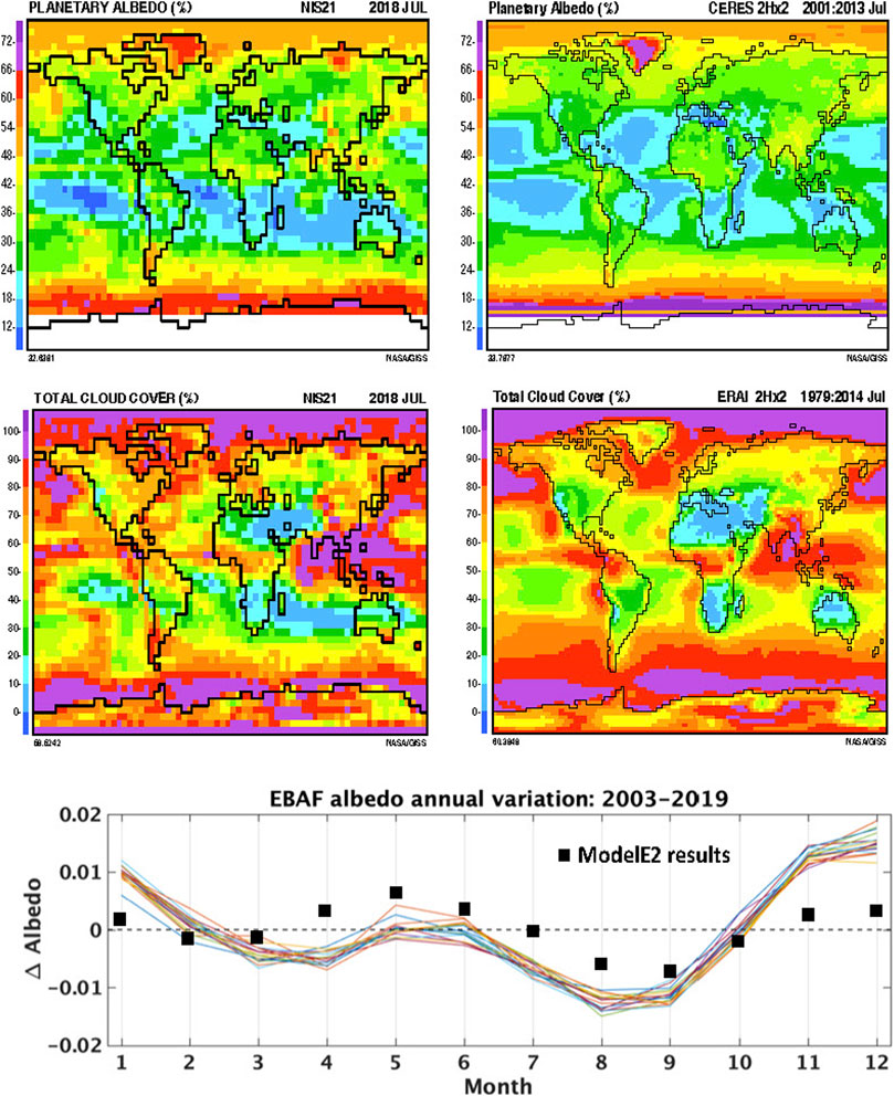
FIGURE 1. ModelE2 4 × 5 degree horizontal resolution monthly-mean planetary albedo (Upper Left) and total cloud cover (Middle Left) computed for July 2018. The corresponding observational counterparts are the CERES planetary albedo (Upper Right) on a 2 × 2.5 degree grid averaged over the years 2001–2013, and the ECMWF Re-Analysis-Interim (ERAI) total cloud cover (Middle Right) also on a 2 × 2.5 degree grid averaged over the years 1979–2014. Seasonal CERES EBAF planetary albedo (Bottom) for 2003–2019 (Loeb et al., 2009; 2018) with the ensemble annual mean subtracted. For comparison, the black squares depict the ModelE2 decadal-mean seasonal variability of the global planetary albedo for years 2000–2010 with the annual mean subtracted.

Epic-Derived Climate Constraint

EPIC makes full-disk images of the Earth’s sunlit hemisphere in 10 narrow spectral band channels with a 1024 × 1024 (download) spatial resolution. Depending on telemetry rate, 13 to 22 images per day are acquired from the Lissajous orbit at the Lagrangian L1 point 1.4 to 1.6 × 10⁶ km from the Earth in the direction of the Sun. The procedure for converting the EPIC spectral radiances into EPIC reflected SW fluxes is described by Su et al., 2018; Su et al., 2020. Using MODIS/CERES-based regression relationships, the spectral radiances are first converted into broadband SW radiances. They are then transformed into radiative fluxes using the CERES angular distribution models. All these tasks are performed at the pixel level, then integrated over the entire sunlit hemisphere (as viewed from the Lagrangian L1 point) to convert each EPIC image into a single climate-style data point for the sunlit hemisphere-mean reflected SW flux. Without loss in precision, these reflected SW fluxes are normalized relative to CERES global annual-mean SW radiative flux (Loeb et al., 2018), and divided by the Total Solar Irradiance (TSI) (Kopp and Lean, 2011) to obtain the planetary albedo.

For each day’s-worth of 13–22 images, the EPIC derived SW fluxes are interpolated to their nearest Greenwich-Mean (GMT) hour to align the data points in longitude. Thus, the 5,000 to 6000 EPIC images per year are transformed into 12 × 24 monthly-mean tables of planetary albedo points, plotted in Figure 2 (Upper). The color-coded longitudes cover the full rotation of the Earth in 1-h time-steps (24 h of GMT, and 15^o steps in longitude). The data are grouped into five broad longitude ranges color-coded as follows: Pacific Ocean (dark blue), East-Asia (green), Africa-Asia (magenta), Atlantic Ocean (light blue), and North America (orange). Key meridians of the five longitude ranges are further identified by their heavier solid color and black dots that depict their monthly-mean value at their mid-month position, which also include the sub-satellite latitude listed at the bottom of the figure. The group members are further identified by a different line-style. Each color-coded meridian is identified by its Greenwich-Mean time (GMT) of noon-time sun. Thus, the international Date Line is identified by its 0 GMT. In addition to the GMT designation, each meridian is also identified by a geographic reference to help identify its relative location.

FIGURE 2

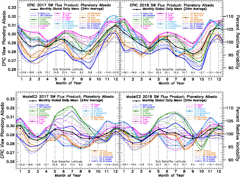
FIGURE 2. Planetary albedo from EPIC reflected SW flux for 2017 and 2018 (Upper Left and Upper Right), normalized by the CERES global annual-mean SW radiative flux (Loeb et al., 2018), and divided by the seasonal Total Solar Irradiance (Kopp and Lean, 2011). The longitudinal slicing is depicted by the colored lines, which represent longitudinally contiguous regions, and which correspond to Greenwich-mean time of high-noon meridians that are also tagged with the geographic location of the illuminated hemisphere-center meridian. The representative members of each colored longitude grouping is identified by its designated black dot monthly-mean position. Geographically, the colored lines proceed westward from the international date line at 1-hourly intervals (15° of longitude). The heavy black line is the daily-mean average over a full rotation of the Earth. The mid-month DSCOVR sub-satellite latitude is depicted at figure bottom. Bottom Left and Bottom Right are the corresponding planetary albedo results for 2017 and 2018 obtained from GISS ModelE2 simulations running with prescribed current-climate sea surface temperatures, and using in-line sampling of the GCM output data using SHS sampling in accord with the DSCOVR Ephemeris viewing geometry.

The key takeaway from Figure 2 Bottom panels is that, over the East-Asia area (3 GMT, black-dot green), ModelE2 overestimates clouds during the NH summer season (since clouds are the principal contributors to Earth’s planetary albedo, e.g., Stephens et al., 2015). Meanwhile, the cloud reflectivity over the continental Africa-Asia land areas (8 GMT, black-dot magenta) is strongly underestimated. By comparison, the EPIC results in the Figure 2 Top panel show planetary albedo to be highest over the Africa-Asia region, in strong contrast to the ModelE2 longitudinal dependence.

A likely explanation for this striking model/data difference is the use of a globally uniform relative humidity criteria for the onset of cloud condensation in the ModelE2 cloud scheme, which involves utilizing a critical (less than 100%) relative humidity criteria for the statistical overlap of water vapor and temperature probability distributions, becoming sufficient to achieve the relative humidity threshold for cloud condensation over some fraction of the grid box. Due to the broader water vapor and temperature probability distributions that exist over land compared to ocean, conditions are more favorable for cloud formation over land compared to the ocean. Thus, using a globally uniform cloud condensation onset will overestimate clouds over the ocean and underestimate clouds over land. Using land/ocean dependent relative humidity criteria to make it more difficult to form clouds over ocean, and easier over land, would lead to improved agreement with observations by reducing the cloud radiative effect over the ocean while increasing the cloud contribution to planetary albedo over land.

Other significant differences are the daily-mean of the seasonal variability depicted by the heavy black line, which resembles the general EPIC data variability, but has less than half of seasonal amplitude of the EPIC planetary albedo, and the ModelE2 planetary albedo during NH summer months, which has little resemblance to the EPIC planetary albedo. However, there is some similarity in that ModelE2 planetary albedo exhibits similar longitudinal ordering and slope during the winter months, from January to March and also from October to December.

The Figure 2 “spaghetti-line” planetary albedo data is shown in Figure 3 in Hovmöller format with the EPIC planetary albedo at figure Left, and corresponding ModelE2 results at figure Right. The Hovmöller format has specific value for displaying space-time variability, whereas the line format provides a more quantitative comparison for the amplitude of the seasonal and longitudinal variability. In the Hovmöller (1949) format, the Y-scale has time increasing upward (with some implicit latitudinal perspective). The X-scale depicts the longitudinal dependence (including the noon-time GMT of EPIC image acquisition). To help locate GMT and longitude points in their geographic perspective, world maps in 4^o x 5^o GCM resolution are displayed in Figure 4.

FIGURE 3

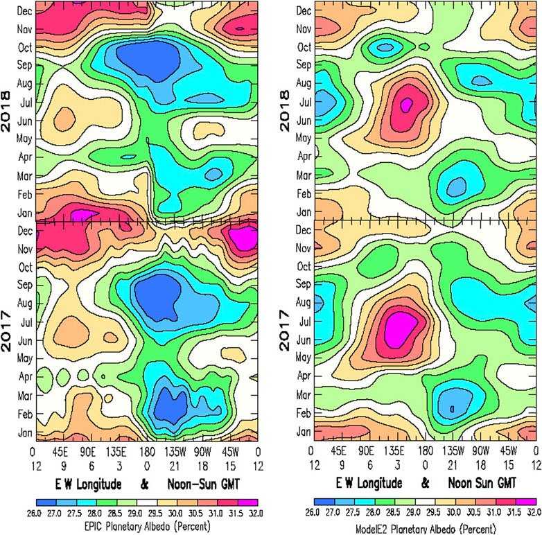
FIGURE 3. Hovmöller plots of the EPIC (Left) and ModelE2 (Right) planetary albedo for 2017 and 2018 for the same data presented in Figure 2. The Y-scale has time running upward starting with January 2017 at the bottom through December 2018 at the top. The X-scale is longitude running from 0° E longitude at the left and 0° W longitude at the right. The X-scale references the GMT of the noon-time Sum, starting at GMT = 0 at the Date Line at the center, proceeding westward toward the left as the Earth rotates. The input data for the Hovmöller plots is precisely the same 12 × 24 tables of monthly-mean sunlit hemisphere averages for the 24 uniformly spaced GMT for both EPIC and ModelE2, respectively. In the color bar, magenta identifies the highest planetary albedos, deep blue the lowest.

FIGURE 4

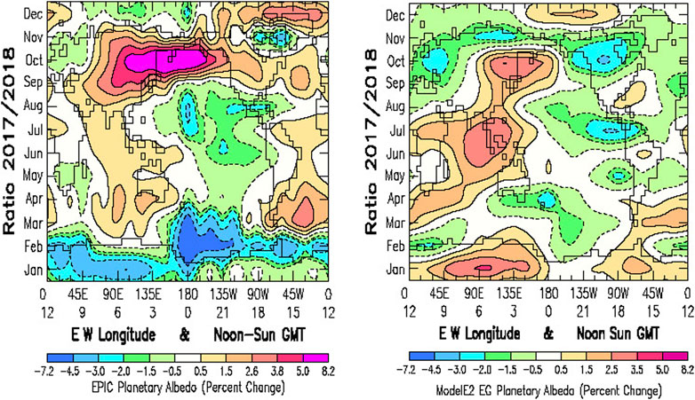
FIGURE 4. Hovmöller-style ratio plot of year 2017 divided by year 2018 of the EPIC (Left) and ModelE2 (Right) planetary albedo plotted in Figure 3. The Y-scale has time running upward starting with January at the bottom through December at the top. As in Figure 3, the X-scale is longitude running from 0° E longitude at the left to 0° W longitude at the right. GMT references the location of high-noon Sun. The world map is included for geographic reference.

Year 2017 has been identified as a La Niña year (Zhang et al., 2019). Presumably related to this, there is the significantly greater space-time variability evident in 2017 than in 2018. Most notable is the sharp decrease in planetary albedo (Figure 3, Bottom Left) over the Central Pacific region during February-March of 2017.

Also remarkable are the enigmatic oscillations (with a peak-to-peak periodicity spanning ∼ 30° in longitude) that appear over the Eastern Pacific in February and November, and over the Indian Ocean in April. In contrast, year 2018 appears to be a uniformly quiescent year having apparently reverted back to ENSO-neutral conditions. As for identifying the geographic epicenter and its spatial extent of the features responsible, that is not within reach, based just on the hemisphere-averaged longitudinal variability information that is available. These features appear to be of limited extent in size and duration in time. Yet their radiative impact is clearly evident on the hemisphere-mean EPIC derived planetary albedo. La Niña activity is identified by fluctuations in sea surface temperature that then induce the atmospheric response in cloud cover. It may be that the space-time variability of the EPIC planetary albedo can serve as an indicator of La Niña/ENSO activity.

The 2017 April oscillations over what is likely the Indian Ocean, are unique in that they are limited in their time duration as well as in spatial extent. Like the February and October-November oscillations in this area, they have peak-to-peak ∼ 30^° extent in longitude, but have a time duration that is only about a month. Their location in longitude extends basically from South Africa to Australia. It is unclear whether these Indian Ocean oscillations might be related to the La Niña phenomenon, or if they are just simply a different member of the ubiquitous climate system oscillations.

Interestingly, there are several longitudes that exhibit extended periods of steady monotonic change in planetary albedo. One such example is the 2017 (and 2018) Atlantic Ocean region, represented by West Africa (13 GMT, black-dot light blue) in Figure 2 Top, and in Figure 3 Left along the GMT = 13 longitude, which has its season minimum planetary albedo in August that keeps increasing steadily through December.

The Figure 3 Right Hovmöller comparison of ModelE2 results to EPIC shows little resemblance, due largely to the overestimated northern hemisphere (NH) summer cloudiness over the East-Asia and Western Pacific, which appear as the isolated large regions high albedo near left-center of the annual panels. Perhaps the most disappointing is the absence in the ModelE2 results of the strong decrease in planetary albedo over the Central Pacific in February is the Figure 3 Bottom Left EPIC results. It is plausible that this might be an artifact due to initialization issues of switching on the prescribed current-climate SSTs for 2017 and 2018 from their climatological spin-up versions, and not allowing sufficient time for the atmosphere and clouds to adjust to the prescribed SSTs. Otherwise, there are only modest perceptible differences between the ModelE2 results for the 2017 La Niña year and 2018. There is little evidence of the persistent oscillations that are so prominent in the EPIC results in Figure 3 Bottom Left.

Figure 4 is a ratio plot of the 2017 and 2018 Hovmöller maps in Figure 3. With 2018 as the reference year, ratioing isolates the La Niña atmospheric (and cloud) response by removing the large seasonal climatological variability. Except for the still glaring absence of the February La Niña signature in the ModelE2 results, there is otherwise substantial agreement in the ModelE2 response to the 2017 La Niña SST changes that are seen in the EPIC results, such as decreased planetary albedo across the Central and Eastern Pacific and increased planetary albedo over the East-Asia region.

Overall, ModelE2 does not reproduce the strong EPIC February decrease in planetary albedo, or the sharp increase in October, which appears to be caused by a shift in the seasonal increase planetary albedo between 2017 and 2018. Also, assuming 2018 to be a ENSO-neutral year, there would appear to be a possible La Niña precursor occurring over the Indian Ocean during January 2017 with a strong decrease in the EPIC planetary albedo.

The “spaghetti” line plots in Figure 2 and the Hovmöller contour maps in Figure 3 are two very different ways to represent and compare precisely the same data, in this case, the tabulated data of longitudinally sliced EPIC planetary albedo and the similarly sampled ModelE2 GCM output data. The data have been strongly averaged, thus making small differences of a percent or less to be meaningful. The Figure 2 line plots provide the more quantitative representation of the differences in the seasonal variability between neighboring longitudes or longitude groups, showing quantitatively the GCM deficiencies in longitudinal cloud distribution.

Clearly, the Figure 3 Hovmöller maps are best in displaying the patterns of variability, showing convincingly the La Niña signature in the EPIC planetary albedo data. And the Hovmöller ratio plots of years 2017 and 2018 in Figure 4, by removing the largest common variability, could readily identify the similarities between the EPIC and ModelE2 planetary albedo results that were not apparent from the Figure 2 or Figure 3 comparisons. This same approach is applicable for examining the patterns of variability of cloud properties to see how they contribute to the planetary albedo.

Epic Hemispheric Composite Data

Since clouds are the principal contributors to planetary albedo, the next step is to access the changes in cloud properties and the cloud distribution that produce the observed variability in planetary albedo. For this purpose, the necessary cloud property data are conveniently available in the form of the EPIC Composite data.

In the process of generating the EPIC-based radiative SW fluxes, Su et al. (2018) constructed the 5-km resolution EPIC composite database, which includes detailed cloud properties such as cloud fraction, cloud-top altitude, and cloud optical depth, water/ice phase, and particle size, compiled from multiple imagers in low earth orbit (LEO) and geostationary (GEO) satellites, with the data selection tuned to closely match the EPIC observations in time and viewing geometry. Monthly-mean and sunlit hemisphere averages are thus available for longitudinal slicing analyses that match those for the radiative fluxes. With the EPIC composite data, it becomes possible to see the actual causes that lead to the radiative climate symptoms.

The key component of this transformation is the 5-km resolution global composite data product with its optimally merged together cloud properties from Low Earth Orbit (LEO) satellites, and from geostationary (GEO) satellites, based on cloud property retrievals using a common set of retrieval algorithms (Minnis et al., 2008; Minnis et al., 2011). The 5-km composite data product is aggregated from LEO/GEO data for closeness in time and viewing geometry to the EPIC observation time, then convolved to the EPIC grid.

Ancillary data, such as surface type, snow/ice, skin temperature, and precipitable water, are also included in the EPIC composite data (Khlopenkov et al., 2017). CERES Edition4 angular distribution models (Su et al., 2015) are then used to compute SW anisotropic factors for converting EPIC broadband radiances into reflected SW fluxes, which are integrated over the sunlit hemisphere to provide a basic calibration reference for NISTAR measurements, and serve as reference for climate GCM longitudinal slicing comparisons.

Figure 5 Top Panel shows the seasonal variability for the EPIC derived all-cloud sky fraction for 2017 and 2018. The highest cloud fractions are found over the Pacific Ocean (22 GM, black-dot blue) and over the East-Asia region (3 GMT, black dot-green), except for the large dip in September-October of 2018 when North America (18 GMT, orange) is surging to its top value in October-November. The lowest cloud fractions are seen over the Atlantic West Africa region (13 GMT, black-dot light blue). We use the term “dayurnal” here to refer to the variability seen at the Lissajous orbital vantage point during a full day’s rotation of the Earth, and “dayurnal mean”, for the average over all 24 longitude views (heavy black line), which is a global dawn-to-dusk diurnal average, given that each longitude view incorporates a range of diurnal samples from the neighboring longitudes, but its viewing locality is at the Lissajous orbit. This is to differentiate this from the term “diurnal mean”, which already has an established meaning of referring to a local 24-h average. The saving grace for using this term, is that the dayurnal mean is identically reproduced for both EPIC and GCM data sampling.

FIGURE 5

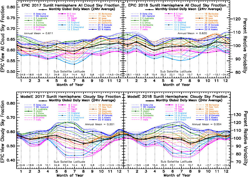
FIGURE 5. All-cloud cloudy sky fraction (Top Panel) from EPIC Composite analysis results for the year 2017 (Top Left) and 2018 (Top Right). (Bottom Panel): All-cloud cloudy sky fraction from GISS ModelE2 SHS in-line sampling results for the year 2017 (Bottom Left) and 2018 (Bottom Right).

The Figure 5 Bottom Panel depicts the seasonal variability of the ModelE2 cloudy sky fraction for the years 2017 and 2018, which corresponds to the EPIC all-cloud sky fraction that is shown in the Figure 5 Top Panel. Here again, the one redeeming feature of the ModelE2 all-cloud sky fraction is that ModelE2 tends to reproduce the overall longitudinal ordering of the EPIC all-cloud sky fraction results, at least in the NH summer months. For ModelE2 and EPIC, the highest cloud fractions occur over East-Asia (3 GMT, black-dot green) and Pacific Ocean (23 GMT, black-dot dark blue) regions, while the lowest occur over Atlantic (13 GMT, black-dot light blue) and Africa-Asia (8 GMT, black-dot magenta) regions. The North America (18 GMT, black-dot orange) meridians are in between, exhibiting a biannual variability with maxima occurring in April-May and in October-November. For ModelE2, the dayurnal amplitude of the seasonal cloud fraction amplitude is at maximum and also at minimum during the NH summer months, with strong constriction of the cloud fraction amplitude, during the NH winter months. Both EPIC and ModelE2 show a small increase in cloud fraction going from 2017 to 2018, with the EPIC cloud fraction increasing by about 1.5%, and ModelE2 by about 0.5%.

Figure 6 displays the cloudy sky fraction data from Figure 5 in Hovmöller format with the EPIC cloud fraction at Figure 6 Left, and the ModelE2 results at Figure 6 Right. The Hovmöller results basically echo the spaghetti line plot results in showing the highest cloud fractions over the Pacific Ocean region with the lowest over the Atlantic, including also much of Europe and Africa and the eastern parts of North and South America.

FIGURE 6

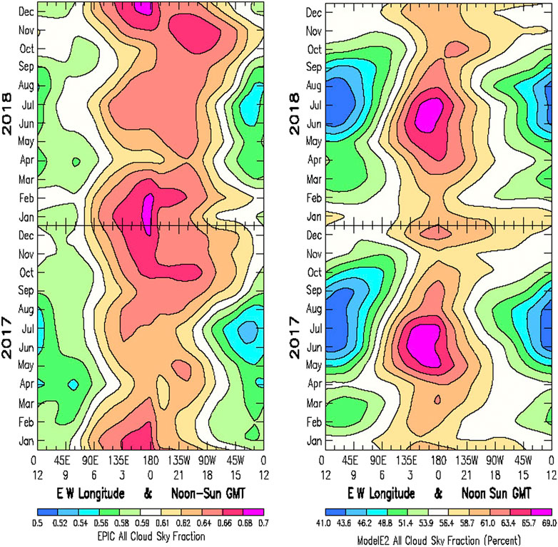
FIGURE 6. Hovmöller plots of the EPIC (Left) and ModelE2 (Right) cloudy sky fraction for 2017 and 2018. The Y-scale has time running upward starting with January 2017 at the bottom through December 2018 at the top. The X-scale is longitude running from 0° E longitude at the left and 0° W longitude at the right. The X-scale references the GMT of the noon-time Sum, starting at GMT = 0 at the Date Line at the center, proceeding westward to the left as the Earth rotates. In the color bar, magenta identifies the highest cloud fractions, deep blue the lowest.

In comparing the EPIC cloud fraction variability between the year 2017 (La Niña) and 2018, there are no significant differences in small-scale fluctuations between the 2 years. Except perhaps for a couple of points in April 2017 that appear to be coincident with similar isolated small-scale points occurring in April 2017 of the EPIC planetary albedo fluctuations in Figure 3, the 2 years are similarly quiescent. Given the totally different nature of these two measurements, it is not necessarily surprising. The EPIC planetary albedo is derived directly from a single set of observed spectral radiances. On the other hand, cloud changes involve more options. For example, with favorable meteorological conditions for cloud condensation, clouds can increase vertically in optical depth, rather than spreading out horizontally. Moreover, for the EPIC cloudy sky fraction, thresholds are involved in deciding whether a given pixel is declared to be mostly clear, or mostly cloudy, and that for some threshold, optically thin clouds might be missed altogether.

For ModelE2, cloud fraction is defined in a still different way. Based on grid-box-mean meteorological conditions, a cloud fraction is determined at each grid box. A random number is then used to decide whether radiative calculations are to be performed for either a totally clear or totally cloudy grid box. Thus, as a computing time saving device, ModelE2 clouds are treated as being fractional in time rather than being fractional in space. Radiatively, for monthly-mean averages, it all averages out. Perhaps it is remarkable that the EPIC and ModelE2 cloud fractions agree as well as they do. As for the strong constrictions in dayurnal amplitude of ModelE2 cloud-top altitude during winter months, there appears to be no explanation.

While changes in cloud-top altitude have only minimal impact on the planetary albedo, they have a profound effect on the outgoing LW radiation due to the direct temperature dependence of thermal radiation that is emitted to space from the cloud-top region. As a result, cloud-top altitude is an important climate variable that is directly involved in defining the Earth’s radiative energy balance, but on the thermal outgoing LW radiation side. Thermal LW radiation is not currently included in the EPIC Composite data collection, so comparing cloud altitude and its LW radiative effects is beyond the scope of this model/data comparison.

Nevertheless, cloud-top altitude is one of the key cloud properties that are tabulated as part of the EPIC Composite Data (Su et al., 2018). The cloud property information is retrieved from multiple imagers in low Earth orbit (LEO) satellites that include MODIS, VIIRS, and AVHRR, and also geostationary (GEO) satellites such as GOES-13, GOES-15, METEOSAT-7, METEOSAT-10, MTSAT-2, Himawari-8. Cloud properties were deduced using a common set of algorithms based on the CERES cloud detection and retrieval system (e.g., Minnis et al., 2008; Minnis et al., 2011). Cloud properties from the LEO/GEO imagers are merged together to provide a global composite data product with 5-km resolution by using an aggregated rating system that optimizes the space-time viewing geometry characteristics to provide the best match with EPIC observations. The global composite data are then remapped into the EPIC grid so as not to degrade the EPIC Composite cloud fraction information (Khlopenkov, et al., 2017).

The Figure 7 Top Panels display the seasonal and longitudinal variability of the EPIC Composite cloud-top altitude. Interestingly, both the highest and lowest cloud altitudes occur in July, and more broadly, during the NH summer months for both 2017 and 2018, when the dayurnal cloud-top amplitude has its largest variability. The highest cloud-top altitudes are experienced over the West China continental region (6 GMT, dot-dash magenta), while simultaneously, the lowest cloud-top altitudes occur over the North America region epitomized by the Iowa (18 GMT, black-dot orange) meridian. The cloud-top minima in the dayurnal amplitude are seen in April and October in 2017, with a somewhat deeper minimum occurring in October-November of 2018. The annual-mean cloud-top altitude remains basically unchanged between 2017 and 2018 (registering a small 1.3% increase).

FIGURE 7

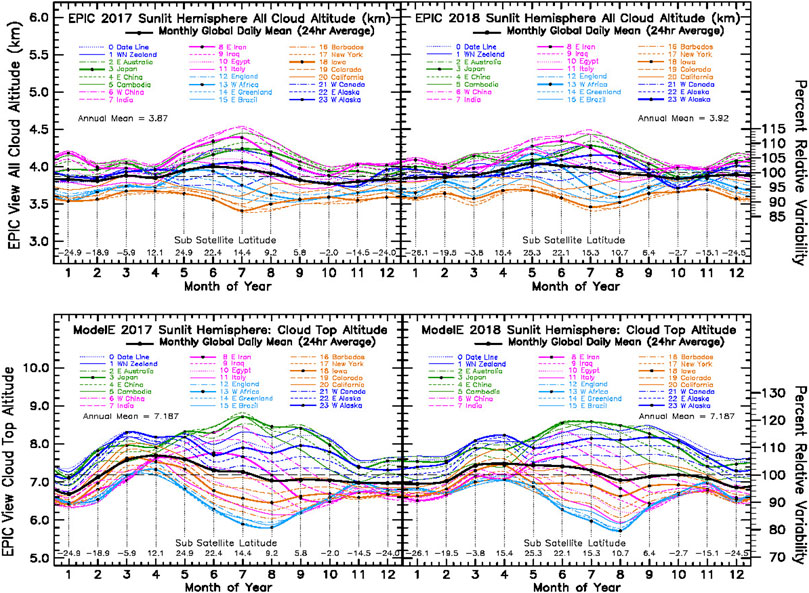
FIGURE 7. Top Panel: All-cloud cloud-top altitude from EPIC Composite analysis results for the year 2017 (Top Left) and for the year 2018 (Top Right). Bottom Panel: All-cloud cloud-top altitude (km) from GISS ModelE2 climate simulations for the year 2017 (Bottom Left) and 2018 (Bottom Right) sampled using the Sunlit Hemisphere Sampling (SHS) simulator and employing the DSCOVR Ephemeris viewing geometry.

The Figure 7 Bottom Panel shows the seasonal and longitudinal variability of the GISS ModelE2 cloud-top altitude. There are some similarities in the overall shape of the seasonal variability of the cloud-top altitude between the EPIC and the ModelE2 results, in that the GCM also has a July centered NH summer maximum, with a mirror minimum, in the cloud-top dayurnal amplitude, but with a more extended (January to May) spring minimum, and a shortened (December) winter minimum. Moreover, there is substantial ramp-up in the dayurnal-mean of the cloud-top altitude from January to April, (heavy black line) followed by a steady deline. The same behavior is seen in the EPIC dayurnal-mean (Top Panel), but with a greatly reduced amplitude. However, the one big difference between the EPIC and ModelE2 cloud-top altitude variability is the difference in the longitudinal ordering. For EPIC, cloud-top altitude maxima are centered over West China (6 GMT, dot-dash magenta), whereas the ModelE2 cloud-top altitude maxima are centered over East-Asia (3 GMT, black-dot green). Similarly, the EPIC, cloud-top altitude minima are centered over North America region epitomized by Iowa (18 GMT, black-dot orange), whereas the ModelE2 cloud-top altitude minima are centered more over the Atlantic Ocean region (13 GMT, black-dot light blue).

The apparent shift in longitude between the cloud-top altitude location between the EPIC observational data and the ModelE2 climate simulation is made far more clearly evident in the Hovmöller representation of the cloud-top altitude variability, as demonstrated in Figure 8. The Hovmöller format shows both the maxima and the minima to be longitudinally aligned, and that his holds for both EPIC (Left) and ModelE2 (Right). For EPIC, the ridge of cloud-top altitude maxima for 2017 and 2018 are persistently located along the 6 GMT (90^° E longitude) meridian running through central Asia (W China). Similarly, a broad valley of cloud-top altitude minima for years 2017 and 2018 are persistently located along the 17 GMT (−75^° W longitude) meridian that runs through New York of the North America longitude group. Extremes in cloud-top maximum and minimum altitudes both occur during the NH summer season centered on July.

FIGURE 8

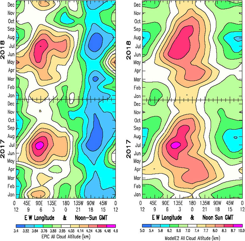
FIGURE 8. Hovmöller plots of the EPIC (Left) all-cloud cloud-top altitude from EPIC Composite analysis results for 2017 and 2018, and ModelE2 (Right) from GISS ModelE2 climate simulations for the years 2017 and 2018, for the corresponding line plots of cloud-top altitude in Figure 7.

A similar pattern in the seasonal and longitudinal variability of cloud-top altitude appears also to hold for ModelE2, as shown in Figure 8 Right. The principal difference is a general eastward shift by about 45^° in longitude of the ridge of cloud-top maxima, and an eastward shift by about 60^° in longitude for the cloud-top minima.

Another difference between EPIC and ModelE2 cloud-top altitude variability is the more limited range of variability for the ModelE2 cloud-top maximum altitudes, and a larger range of variability for the cloud-top minimum altitudes, compared to EPIC.

Perhaps the biggest difference, but also one of less significance, is the large difference in the cloud-top altitude depicted in Figure 7, which shows the mean cloud-top altitude for EPIC to be about 4 km, while the average cloud-top altitude for ModelE2 clouds is about 8 km. The reasons for this difference arise from the limited ability of satellite remote sensing measurements to detect optically thin clouds, and also the retrieved, or inferred, cloud-top altitude refers to the optical depth τ = 1.0 level. For ModelE2 clouds, cloud-top pressure is known precisely for all of the model generated clouds, which includes significant numbers of optically thin (τ < 0.1) high altitude cirrus clouds (that automatically constitute the grid-box cloud-top). Also, since the ModelE2 diagnostics assign the cloud layer’s top edge as the cloud-top, this is setting the ModelE2 cloud top at the optical depth τ = 0 level, which further biases higher the ModelE2 cloud-top results. Since all of the ModelE2 cloud optical depth information is available at the SHS diagnostic data sampling aggregation, it should be possible to establish a thin-cloud threshold, compute the optical depth τ = 1.0 level, and re-define the ModelE2 cloud-top altitude to more closely coincide with the observational cloud-top data.

Also of interest, because the EPIC Composite LE/GEO cloud products are retrieved separately for liquid water and ice clouds (Minnis et al., 2021), the differences in the seasonal and longitudinal variability for the ice cloud the water cloud altitude can thereby be also examined separately, as done in Figures 9, 10.

FIGURE 9

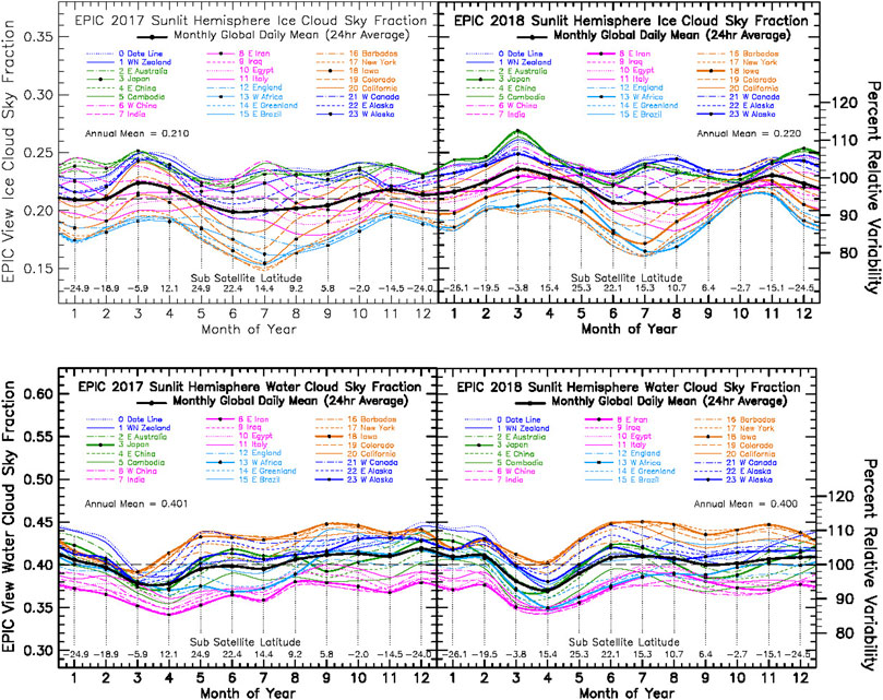
FIGURE 9. Top Left: Ice cloud sky fraction from EPIC Composite analysis results for year 2017, and Top Right: ice cloud sky fraction for year 2018. Bottom Panel Left: Water cloud sky fraction from EPIC Composite analysis results for year 2017, and Bottom Right: water cloud sky fraction for 2018.

FIGURE 10

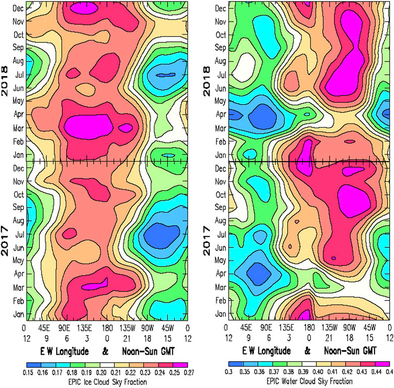
FIGURE 10. Left: Hovmöller format ice cloud sky fraction from EPIC Composite analysis results for the year 2018 (Upper Left) and 2017 (Lower Left). Right Panel: Water cloud sky fraction from EPIC Composite analysis results for the year 2018 (Upper Right), and for year 2017 (Lower Right).

Epic Composite: Ice and Water Clouds

In addition to the all-cloud category, the EPIC Composite database also separates clouds into ice cloud and water cloud categories. The GISS ModelE2 also generates ice and water clouds, with precise internal knowledge of the ice and water cloud radiative properties and distribution. But due to unbridgeable differences in definition, direct comparison of the EPIC and ModelE2 ice and water cloud properties is not warranted, as this could lead to false conclusions. The EPIC Composite ice/water cloud differentiation is tied to the Minnis et al. (2021) retrieval algorithms that are used in CERES and MODIS retrievals, and this differentiation would be difficult to reproduce from within the GCM output data. Accordingly, the EPIC/ModelE2 cloud property comparisons have been limited just to the more physically based all-cloud sky fraction and cloud altitude.

Thus, it makes good sense to intercompare the EPIC Composite ice cloud and water cloud properties against each other, with the caveat that an increase in ice cloud fraction could have come at the expense of a decrease in water cloud fraction, and vice versa. The same algorithms have been applied uniformly for years 2017 and 2018, so the relative changes should be meaningful. Clearly, the La Niña event has significantly disrupted the cloud distribution, so it is of interest to see how the clouds have changed between 2017 and 2018, even if just from the EPIC Composite data. Bender et al.

(2017) have demonstrated the existence of a convincingly strong positive relationship between cloud albedo and cloud fraction, i.e., that cloud albedo increases with increasing cloud fraction, and that the increase in cloud albedo becomes increasingly greater as the cloud fraction approaches unity, although this relationship does not have an explicit dependence on cloud optical depth.

Figure 9 Top shows the seasonal variability of the EPIC ice cloud fraction, with Figure 9 Bottom showing the corresponding water cloud variability. Compared to the roughly uniform all-cloud sky fraction in Figure 5 Top, counter-acting changes are seen during January-March with the ice cloud fraction increasing and the water cloud fraction decreasing in both 2017 and 2018. Interestingly, the longitudinal ordering of the ice cloud dayurnal variability exhibits similarity to the ModelE2 all-cloud fraction longitudinal variability (Figure 5 Bottom) with the East-Asia (3 GMT, black-dot green) and Central Pacific (23 GMT, black-dot blue) regions near the top, and the Atlantic region (13 GMT, black-dot light blue) near the bottom. Also, there is some tendency for the dayurnal range of the EPIC ice cloud fraction variability to ‘bulge’ in the NH summer months, like the ModelE2 results, with both the maximum and minimum occurring in July. Perhaps most notable is the strong constriction in the ice cloud dayurnal amplitude in November 2018, which again shows some similarity to the ModelE2 results.

A broad range of longitudes from the Date Line 0 GMT, blue dot line) to India (7 GMT, long dash magenta line) appear near the top of the ice cloud sky fraction in Figure 9 Top. It is of interest that the East-Asia (3 GMT, black-dot green line) and Central Pacific (23 GMT, black-dot blue) regions also exhibit some of the sporadic small-amplitude 60-days oscillations during January-March of 2017 and 2018, and from August to December of 2017. Longer periods of 4-to-6-months duration, are also evident in this longitude region. More specifically, the Date Line longitude (0 GMT, blue dot line) appears to be aliasing the changing land/ocean fraction, which is being sampled on 1-h intervals as the Earth rotates (described in more detail in Figure 15). Also prominent in Figure 9 Top is the long period ice fraction variability over the West Africa region (13 GMT, black-dot light blue line), which exhibits the lowest cloud fractions, and is interrupted by some low-amplitude shorter-period 60–90-days oscillations from November 2017 to April 2018.

On the other hand, for the water cloud sky fraction in Figure 9 Bottom, shows that for the most part, the North America region Iowa (18GMT, black-dot orange line) exhibits the largest water cloud sky fraction from 2017 through 2018, and that similarly the Africa-Asia, East Iran region (8 GMT, black-dot magenta line) displays the lowest water cloud sky fractions. Both of these regions also exhibit a couple of the low-amplitude 60-days oscillations from October 2017 to April 2018, with the Date Line longitude (0 GMT, blue dot line) also popping up to the top during this time period. Figure 9 Bottom shows a strong decrease in the water cloud sky fraction centered on March in 2017 for essentially all longitudes, broadening toward April in 2018. The EPIC water cloud fraction accounts for ∼ 2/3 of the all-cloud sky fractions.

Figure 10 shows the seasonal and longitudinal variability of the ice cloud (Left) and water cloud (Right) sky fraction expressed in Hovmöller format. The Hovmöller plots show a clear separation in longitude of the ice cloud and water cloud sky fraction regions of maximum concentration, with the ice cloud sky fraction favoring the longitudes spanning the Indian Ocean, East-Asia, and Central Pacific Ocean, from roughly 45E to 135W. The water cloud sky fraction dominates from the Eastern Pacific (135W to the North and South America continent longitude (45W). The maximum in ice cloud sky fraction occurs in March, with March 2018 being considerably more intense than March 2017. Consistent with the counteractive nature of the ice/water cloud phase determination, the ice cloud maxima coincide with the prominent breaks in the column of the water cloud sky fraction in March 2017 and again in March 2018. As noted in Figure 9 Top, the ice cloud sky fraction increased by nearly 5% from 2017 to 2018, In contrast, Figure 9 Bottom shows essentially no change in the annual mean of the water cloud sky fraction from 2017 to 2018, though there are substantial changes in the longitudinal distribution of the water cloud sky fraction. There is the appearance of a parallel longitudinal column along the Central Pacific Date Line (0 GMT) with less intensity but greater seasonal variability than along the principal water cloud longitudinal column along 90W (18 GMT). Also of note is the relative minimum in the ice cloud longitudinal column occurring in May of 2017 and 2018 when the DSCOVR Spacecraft is at its northern-most position viewing the maximum in land fraction. During December-January, when the Spacecraft is viewing maximum ocean fraction (at 0 GMT), the water cloud sky fraction appears to have a local maximum.

Figure 11 Top shows the seasonal variability in ice cloud altitude for the years 2017 and 2018. There is an overall smoothness and symmetry in the seasonal cloud-top altitude change with a broad NH summer maximum occurring in July and a small secondary SH summer maximum in January, with remarkably little change between 2017 and 2018. The Africa-Asia region, as epitomized by India (7 GMT, long-dash magenta) and East Iran (8 GMT, black-dot magenta), has the highest ice cloud altitude. This is followed by East-Asia (3 GMT, green), Pacific (22 GMT, blue), and Atlantic (13 GMT, light blue), with the North America (18 GM, orange) exhibiting the lowest cloud-top altitude. The same longitudinal order holds for 2018, but with some distortion in the winter months.

FIGURE 11

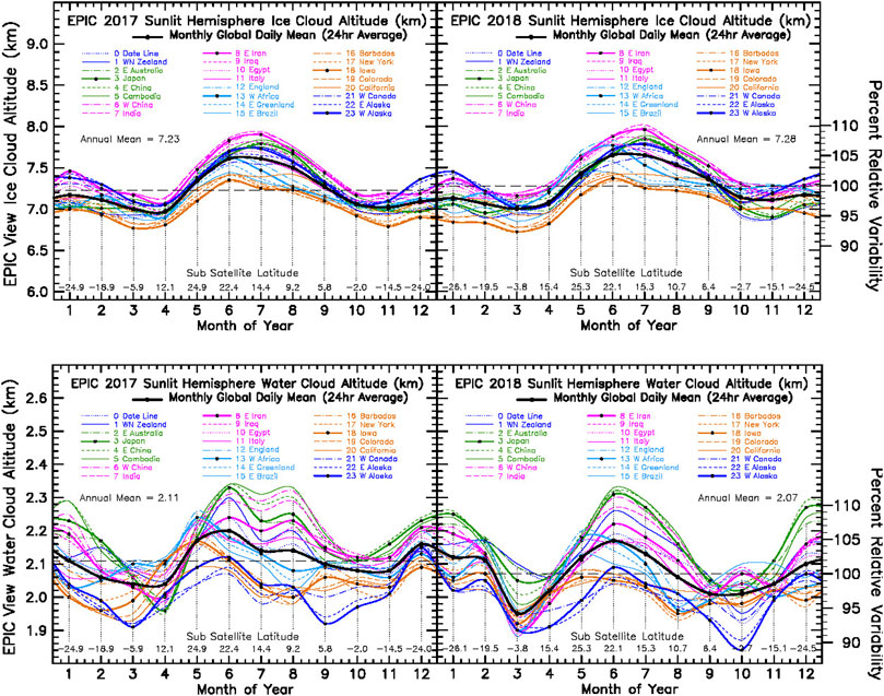
FIGURE 11. Top Left: Ice cloud altitude from EPIC Composite analysis results for the year 2017, and Top Right: ice cloud altitude for the year 2018. Bottom Panel Left: Water cloud altitude from EPIC Composite analysis results for the year 2017, and Bottom Right: water cloud altitude for 2018.

Figure 11 Bottom shows the corresponding seasonal variability of the water cloud-top altitude, which, in contrast to the ice cloud altitude, exhibits more chaotic variability, especially for year 2017, which has been identified as the La Niña year. The water cloud altitude has a broad NH summer maximum with a secondary SH summer maximum in January, thus exhibiting what appears to be a biannual oscillation in global cloud structure. The minima in the water cloud-top altitude occur in March-April and in October, which is the same as the ice cloud seasonal pattern. In 2018, the water cloud summer maximum narrows, and the minima become deeper and broader.

The longitudinal ordering of the water cloud-top maximum has East-Asia region as represented by Cambodia (5 GMT, green) and East China (4 GMT, dash green), at top, followed by neighboring West China (6 GMT, dot-dash magenta) and India (7 GMT, dash magenta), with the minima in water cloud altitude occurring over the East Pacific region, as represented by West Alaska (23 GMT, black-dot blue). The raggedness in the 2017 water cloud altitude variability might be indicative of potential La Niña related activity that is not present in 2018, but the ice cloud shows no such change.

Figure 11 shows some traces of low-amplitude 60-days oscillations in ice cloud altitude, at a number of longitudes from October 2017 to April 2018, with many being 180° out of phase with each other. Perhaps the most persistent are the low-amplitude oscillations over the North America region (18 GM, black-dot orange) beginning in April 2017 and continuing through 2018. Figure 11 Bottom shows similar 60-days oscillations at multiple longitudes, but with a somewhat larger amplitude, the most prominent of those being over the longitude range from New Zealand (1 GMT, solid blue) to India (7 GMT, long dash magenta) from June to August of 2017. There are also oscillations in the January-March time period that might be related to the EPIC La Niña planetary albedo variability. In any case, there are far more of the low-amplitude 60-days oscillations in the 2017 water cloud altitude variability than in non-La Niña 2018.

Nevertheless, representing the water cloud altitude variability in Hovmöller format in Figure 12 does not significantly enhance its discrimination capability to distinguish between the 2017 La Niña conditions and the 2018 non-La Niña conditions the same way that the Hovmöller format could enhance the EPIC planetary albedo in Figure 3 relative to Figure 2. The purported La Niña discrimination in Figure 12 Bottom Right panel does exhibit more variability in 2017 than in 2018, but that variability occurs more along the time dimension than in longitude.

FIGURE 12

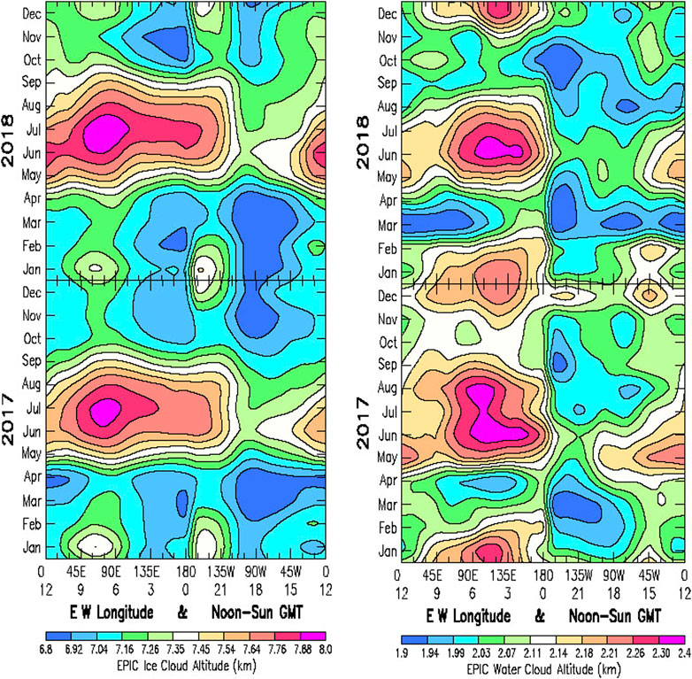
FIGURE 12. Left: Hovmöller format ice cloud altitude from EPIC Composite analysis results for the year 2018 (Upper Left) and 2017 (Lower Left). Right Panel: Water cloud altitude from EPIC Composite analysis results for the year 2018 (Upper Right), and for year 2017 (Lower Right).

However, what does seem to be more unusual about Figure 12, is the near-vertical alignment along longitude lines, as well as also the strong seasonal alignment. The ice cloud altitude in Figure 12 Left shows islands of secondary cloud altitude maxima occurring in December-January along the 7-to-8 GMT and the 22-to-23 GMT longitudes. December-January is the time when the EPIC-view is focused most strongly on Antarctica. The 7-to-8 GMT and the 22-to-23 GMT time periods correspond to the longitudes of maximum and minimum planetary albedo in Figure 2 Top, respectively. The seasonal islands of the strong NH summer maxima in 2017 and 2018 both exhibit a steep rise to maximum in May, and an equally steep decline in August-September. There is a similarly steep longitudinal gradient for these NH summer maxima the extends from May on to September at their eastern edge at 120° W longitude, while tapering off more gradually at their western edge, after spanning nearly the entire globe. Broad regions of ice cloud minimum altitude extend from October to April of the following year. They appear to be offset from the longitude of ice cloud maxima by essentially 180°. The ice cloud altitude variability shows little change between 2017 and 2018, except for the increase in June over England (0 GMT).

On the other hand, it is the water cloud altitude (Figure 12 Right) that exhibits the more significant features that differentiate the La Niña year 2017 from 2018. Most noticeable are the 60-days (time dependent) oscillations that occur during March to August of 2017 over a broad swath of longitudes reaching from the Central Pacific to the Indian Ocean (0–9 GMT). These are the same time dependent oscillations that were readily identifiable in the line plot in Figure 11 Bottom. There appears to be some degree of correlation of this time dependent variability of the water cloud altitude with the water cloud sky fraction variability in Figure 9 Bottom Left, and in Figure 10 Bottom Right, but not with the EPIC planetary albedo variability in Figure 3 Bottom Left. Also, the prominent February-March longitudinal variability feature in the EPIC planetary albedo, is absent in the water cloud altitude plot, but still coinciding the overall space-time location of this feature.

There is the additional June-July longitudinal wave feature in Figure 9 Bottom Right, appearing over the Eastern Pacific Ocean with peak-to-peak variability (17–21 GMT) extending over 7,000 km. Similar variability in water cloud altitude also appears in the year 2018 in March-April, also over the Eastern Pacific Ocean region.

However, the most curious feature of the water cloud altitude variability is the apparent longitudinal discontinuity at the 0 GMT Date Line, with the water cloud altitudes rising steeply to the west, and decreasing steeply to the east. If this were really real, it would require an explanation as to the underlying cause. It is also possible that this demarcation might be a selection criteria artifact in the EPIC Composite data matching process that switches between the different LEO/GEO data sources to select the closest match to the EPIC image time and viewing geometry.

The artificial-looking demarcation and longitudinal alignment along the 0 GMT meridian that stands out prominently in Figure 12 Right, is evident, a least to some extent, in previous Hovmöller plots of EPIC data, such as the sharp longitudinal gradient in the planetary albedo near the 0 GMT meridian during January-March of 2018 in Figure 3 Left, but is not reproduced in the Hovmöller ratio plot in Figure 4 Left. This appears to be an interpolation bias that arises from interpolating EPIC image data points to a uniform GMT grid. Due to telemetry limitations, there are only 13 EPIC images on some days, instead of the normal 22 images per day, which creates wider data gaps in the 0 GMT vicinity that need to be bridged. This interpolation bias persists from year to year and appears to be more pronounced for larger gradients near 0 GMT.

The basic objective of the Hovmöller ratio plots is to isolate the atmospheric and cloud property changes that take place between the 2017 (La Niña) and 2018, by removing the common seasonal and longitudinal variability due to the Lissajous orbital perspective, as well as the surface contributions from Antarctica and continental boundaries that undergo little change. In the process, data artifacts common to both years are also eliminated.

The Hovmöller ratio plots in Figure 13 show little evidence of longitudinal demarcation for the EPIC Composite ice cloud and water cloud sky fraction and cloud altitude results from Figures 10, 12. Figure 10, with cloud fraction uniformity near 0 GMT, had little evidence of longitudinal artifacts from the start. The presence of strong cloud fraction gradients and longitudinal artifacts near 0 GMT in Figure 12, and their elimination by the Hovmöller ratioing tends to confirm their nature as interpolation biases.

FIGURE 13

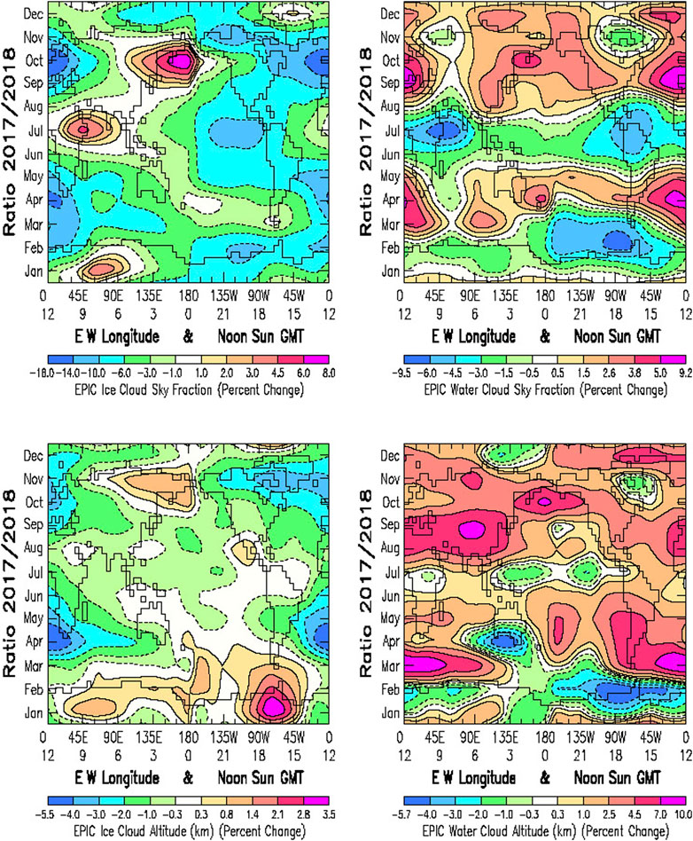
FIGURE 13. Hovmöller ratio contour plots of the percent change for year 2017 relative to reference year 2018 of the EPIC Composite cloud property data for: Upper Left: the ice cloud sky fraction for years 2017/2018 from Figure 10 left; Upper Right: the water cloud sky fraction for 2017/2018 from Figure 10 right; Lower Left: the ice cloud altitude (km) for years 2017/2018 from Figure 12 left; Lower Right: the water cloud altitude (km) for 2017/2018 from Figure 12 right.

The Hovmöller ratio plots for the individual EPIC Composite ice cloud sky fraction and altitude (Figure 13 Left, Top and Bottom), and the water cloud sky fraction and altitude (Figure 13 Right, Top and Bottom), are directly comparable to the Figure 3 EPIC planetary albedo Hovmöller ratio. These four individual cloud components show significant variability and have only several features that coincide with the EPIC planetary albedo features. Moreover, they have but a few features that coincide with each other, and show nothing that might resemble a La Niña signature. Yet, acting together, they must reproduce the space-time variability of the planetary albedo, demonstrating convincingly that independent component comparisons are no substitute for a wholistic quantity.

The Hovmöller ratio plot in Figure 14 Left is the 2017/2018 ratio of the all-cloud EPIC Composite sky fraction from Figure 6 Left, which is also the combined result of the individual ice cloud and water cloud sky fraction components from Figure 13 Top. The EPIC Composite database contains only the all-cloud and the ice cloud components. Given that it is a binary choice for database clouds to be either ice or water cloud, the water cloud variable is defined as a separate entity by the difference between the all-cloud and the ice cloud categories.

FIGURE 14

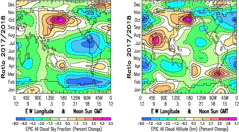
FIGURE 14. Left: Hovmöller ratio plot of the percent change for year 2017 relative to reference year 2018 for the all-cloud sky fraction, combining the results of the separate ice cloud and water cloud sky fractions in Figure 13, top left and top right, respectively. Right: All-cloud sky fraction, combining the results of the separate ice cloud and water cloud altitude in Figure 13, bottom left and bottom right, respectively.

Interestingly, the all-cloud sky fraction ratio in Figure 14 Left compares far more favorably with the EPIC planetary albedo ratio (Figure 3 Left) than the ice cloud and water cloud sky fraction ratios considered separately as in Figure 13 Top. The two most prominent features of the EPIC planetary albedo ratio are the strong February albedo decrease stretching from 180° W to 0° W longitude, and the strong October increase in albedo that stretches from 90° E to 135° W longitude. Both of these year-2017 “La Niña” features are reproduced in the all-cloud sky fraction ratio plot, especially the February strong decrease in sky fraction, also stretching from 180° W to 0° W longitude. Since cloud fraction correlates well with cloud albedo (Bender et al., 2017), these changes in cloud fraction are consistent with the space-time changes in the EPIC planetary albedo variability. However, there is an additional “strong decrease in all-cloud sky fraction” occurring in July from 135° W to 45° W longitude in the all-cloud fraction ratio, which has no similar feature in the EPIC planetary albedo ratio.

Similarly, the all-cloud altitude ratio in Figure 14 Right also compares far better with the EPIC planetary albedo ratio pattern of variability than the separate ice cloud and water cloud altitude ratios shown in Figure 13 Bottom. The improved agreement is not specifically in achieving a closer match-up for the principal features, but rather in a more general alignment of the peripheral pattern of variability surrounding a more or less quiescent Pacific Ocean region during the April to September time period. Since the cloud altitude change by itself has only minimal impact on the planetary albedo, the actual improvements in agreement with the planetary albedo variability patterns must originate from radiative effects that arise from changes in the other accompanying cloud properties. The cloud altitude changes would more directly affect the outgoing LW thermal radiation, which may potentially have its own unique “La Niña” response signature.

Despite the apparent agreement of the all-cloud sky fraction in reproducing the principal February decrease in planetary albedo, there is a potentially significant difference in that the prominent 30° period longitudinal oscillations in the EPIC planetary albedo variability, which, except for the interval from 45° E to 180° E, effectively span the entire globe, but which are not reproduced in the all-cloud sky fraction variability. It may be that the reason for this is due to differences in data resolution. The EPIC planetary albedo, or rather the reflected solar SW radiance measurements at the pixel level are unitary wholistic measurements that record and tabulate the reflected radiances at a high digital resolution. Cloud cover, on the other hand, is the result of a binary decision of clear of cloudy, depending on some arbitrary threshold. There is no way for the retrieval algorithm to know if at the sub-pixel level, the entire pixel is filled with an optically thin cloud, or if it is only a small fraction of the pixel that may contain an optically thick cloud. Thus, it may be that for reflected solar SW radiation, as a unitary wholistic measurement, tiny changes that contain the global-scale oscillation signal can be reliably tabulated and recorded across the entire sunlit hemisphere, whereas such tiny changes that might be present in the different cloud properties, never get a chance to be tabulated by getting wiped out by the clear/cloudy threshold.

From the foregoing, it appears that it may be the unitary wholistic nature of the EPIC radiance measurements that enable the planetary albedo data to provide the best representation for comparing the year-to-year space-time variability that may be contained within the sunlit hemisphere EPIC measurements. Such comparisons of year-to-year changes in the EPIC data planetary albedo are being examined here to see if characteristic differences can be identified between 2 years of data, such as the 2017 La Niña year and 2018, which is representative of more ENSO-neutral conditions. While cloud radiative properties may be the fundamental building blocks of the planetary albedo, cloud properties do not vary lockstep as clouds change in the climate system. Thus, selection of a cloud property to serve as an indicator in the year-to-year comparisons does not lead to greater clarity in interpretating the comparison results, but rather serves to magnify the diversity of the different cloud property radiative effects. Knowing quantitatively how the different cloud properties contribute toward the planetary albedo is important in itself, but the planetary albedo is also robust as a measure of the Earth’s global energy balance.

The changing DSCOVR-view Lissajous orbital perspective of the EPIC data is a significant contributing factor to the seasonal and longitudinal variability that is seen in the longitudinal slicing comparisons of EPIC and ModelE2 data. Averaging data over the Earth’s sunlit hemisphere averages out meteorological weather noise as well as the latitudinal and longitudinal information. The rotation of the Earth retrieves the longitudinal component of the planetary scale variability via longitudinal slicing. Likewise, some significant fraction of the latitude dependent information is retained by the combined change in solar declination and the Lissajous orbital motion of the DSCOVR Satellite as depicted by the sub-satellite latitude at figure bottom (Figure 15 Top) that is varying from its southern extreme position in January, to its northern extreme in May, and then back to its southern extreme in December.

FIGURE 15

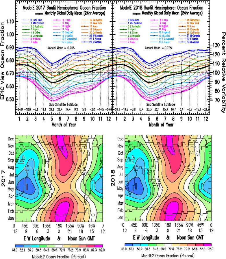
FIGURE 15. Upper Left: Line plot of the ModelE2 ocean fraction for the year 2017. Upper Right: Line plot of the ModelE2 ocean fraction for the year 2018. Lower Left: Hovmöller contour map of the ModelE2 ocean fraction for year 2017. Lower Right: Hovmöller contour map of the ModelE2 ocean fraction for year 2017. The seasonal change in ocean fraction is due to the DSCOVR Spacecraft Lissajous orbital motion as denoted by the Sub-Satellite latitude at figure bottom. The tiny differences in the line and Hovmöller plots between years 2017 and 2018 arise from the slow orbital drift of the DSCOVR Spacecraft in its Lissajous orbit.

The land/ocean fraction is another significant contributor to the seasonal and longitudinal variability in the longitudinal slicing comparisons of EPIC and ModelE2 data. Except for a small seasonal change in sea ice, the ocean fraction is static in time. Hereby, we identify and quantify the net effect that these otherwise invariant contributors have on the line format and Hovmöller contour map comparisons between the EPIC observational, and the ModelE2 climate GCM results for planetary albedo and cloud properties.

Figure 15 Top is the line plot of the (static) ocean fraction for years 2017 and 2018. As to be expected, the Pacific Ocean region (black-dot blue) corresponds to the largest ocean fraction, and the Africa-Asia region (black-dot magenta) the smallest with the Atlantic region (black-dot light blue) nearby. The East Asia (green) and the North and South America regions (orange) undergo significant seasonal variability, showing time dependent oscillations of 4-to-6 months duration, in particular during the July to November time frame. More importantly, the dayurnal and seasonal variability of the ocean fraction does not generate the higher frequency 60–90 days oscillations that are abundantly present in the EPIC planetary albedo and cloud property data.

Figure 15 Bottom shows the Hovmöller contour map of the (static) ocean fraction for year 2017 (Left) and for 2018 (Right). The objective of these plots is to show that while the seasonal effects of the Lissajous orbital and solar declination motion are significant, the effect of the year-to-year Lissajous orbital shift is practically imperceptible. The minimum ocean fraction occurs in May over Iraq (9 GMT). With world map superimposed, the time dependent oscillations in the line plot are visible in the East Asia region from May to September, as is the constriction in ocean fraction near the 0 GMT Date Line. No longitudinal oscillations are discernable.

Discussion

The current model/data comparison study arose from a brute-force effort to calibrate the NISTAR Band-B full-disk sunlit hemisphere measurements. Fully calibrated; with the ability to reliably convert near-backscattered radiances into SW fluxes, NISTAR data would, on their own, be able to reproduce the EPIC planetary albedo results in Figures 2, 3. To this end, Su et al. (2018) converted the EPIC image 1024 × 1024 narrow-band, backscattered radiances into the 12 × 24 tables of monthly-mean, SW reflected hemisphere-mean fluxes for years 2017 and 2018, that constitute the planetary albedo comparisons of this study.

Spectral radiances from 5388 EPIC images for 2017, and 5,351 for the year 2018 were processed and converted into the 12 × 24 (monthly-mean, GMT-hourly) tables of reflected SW fluxes. The EPIC-viewable sunlit-hemisphere fractions generated annual-means of 204.63 and 202.90 Wm⁻², respectively, with ∼ 1.0 Wm⁻² standard deviation. The EPIC Composite cloud properties have similar data reliability out to the third decimal. Because of Lissajous orbital motion, the EPIC-viewable fraction of the sunlit disk varies from ∼ 92 to ∼ 97 percent of the full disk, introducing some uncertainty as to the total full disk reflected radiation. Accordingly, both the EPIC and the ModelE2 annual-mean planetary albedo have been normalized to the 29.1% CERES value (Loeb et al., 2018) to focus more on comparing the space-time patterns of variability rather than interannual change.

Moreover, it is important to note that planetary albedo contains both atmospheric and surface contributions. The DSCOVR vantage point combined with the seasonal change in the tilt of the Earth’s rotational access results in a time changing contribution from the polar regions which maybe further enhanced in the EPIC observations due to the backscatter viewing geometry. Explicit treatment of the scattering enhancement at near back-scattering angles introduces an uncertainty in both the calculation of the shortwave flux from the EPIC observations and the model. Thus, while the signature of these surface contributions is apparent in the figures shown in this paper, quantitative evaluation of these surface driven model/observation differences requires additional research and is beyond the scope of this investigation. To ensure that we are not mixing this type of surface contribution into our analysis, we examine the ratios two individual years since orbital and surface contributions will be minimized allowing us to focus on the atmospheric changes.

With quasi-chaotic meteorological weather-scale noise averaged out, the EPIC and the similarly sampled ModeE2 data are uniquely positioned for a climate-style model/data comparison with excellent space-time data sampling self-consistency. EPIC image acquisition on the near-hourly basis coincides closely with the climate GCM (GISS ModelE2) 1-h radiation time-step radiation calculations that are performed ‘instantaneously’ for all GCM grid boxes.

The only real requirement on the part of the GCM in the sunlit hemisphere averaging of output data, is to use Solar and DSCOVR Satellite Ephemeris information to impose Lissajous orbital viewing geometry and projected area weighting of the individual grid box contributions to the sunlit hemisphere average. All this ensures that the diurnal cycle is sampled the same way by the GCM as by EPIC, with high noon sub-satellite meridian, and sliding noon-to-dusk, and noon-to-dawn, diurnal contributions from neighboring longitudes to east and to the west, properly aggregated.

In this way, weather noise and the latitudinal and longitudinal dependence in the sunlit hemisphere are averaged out. Differences in spatial resolution between the EPIC and GCM data are similarly side-stepped. Remaining in the data is the seasonal and planetary scale variability. Longitudinal dependence is made accessible by the rotation of the Earth. Some latitudinal dependence is captured by the seasonal change in solar declination and also as a result of the Lissajous orbital motion of the DSCOVR Satellite.

The Figure 2 line plots are the first longitudinal slicing EPIC and ModelE2 planetary albedo comparisons, showing the seasonal change in dayurnal variability of the planetary albedo in 1-hourly time-steps as the Earth rotates. The immediate take away of this comparison is that while the overall envelope of planetary albedo variability is comparable, the ModelE2 dayurnal amplitude is too large during the northern hemisphere (NH) summer months and too small during the winter months, and it is only during the winter months that the longitudinal ordering of the dayurnal variability matches that of EPIC.

The biggest mismatch is that during the NH summer months, ModelE2 significantly overestimates the planetary albedo, hence clouds, over the ocean areas, and underestimates clouds over the continental land areas. This was a problem stemming from the use of a globally uniform relative humidity threshold in ModelE2 that the GISS GCM modeling group had been aware of, and have already implemented a rigorous physics-based cloud treatment for the GISS ModelE3 version. The Figure 2 comparison makes this a quantitative climate GCM performance diagnostic showing the largest overestimate to be over the East-Asia region (3 GMT, black-dot green line), while the EPIC data show t the maximum NH summer planetary albedo to be occurring instead over the continental Africa-Asia region (8 GMT, black-dot magenta line).

The model used in this study was the GISS coarse-grid coupled atmosphere-ocean 4^° x 5^° ModelE2 version (Schmidt et al., 2014), utilizing a mass-flux cumulus parameterization that is based on a cloud base neutral buoyancy flux closure originally described by Del Genio and Yao (1993), with stratiform clouds based on a Sundqvist-type prognostic cloud water approach, with diagnostic cloud fraction (Del Genio et al., 1996). Tuning is used to bring the empirical parameterizations of physical processes in acceptable agreement with observations (Schmidt et al., 2017). This involves establishing a critical relative humidity criteria for the onset of cloud condensation in a GCM grid box, based on the statistical overlap of water vapor and temperature probability distributions to achieve relative humidity conditions for cloud condensation.

Replotting the planetary albedo data in Hovmöller format in Figure 3 Left produced an unexpected result by bringing out detail in the EPIC planetary albedo variability that was not apparent in the Figure 2 line plots. It turns out that there is far more of the characteristic (monthly, and 30^° longitude) variability in planetary albedo in year 2017, compared to the more quiescent appearance in 2018. Most notable it the strong decrease in planetary albedo during February 2017 over the Central Pacific Ocean longitudes.

This difference in planetary albedo variability between the years 2017 and 2018 is further enhanced and isolated to atmospheric changes by the 2017/2018 Hovmöller ratio plot in Figure 4 Left, by canceling out the seasonal variability patterns that are common to both years (e.g., the surface contribution from Antarctica shown by the magenta areas in Dec/Jan evident in the upper left of the two right panels of Figure 3). The sharp February decrease in the EPIC planetary albedo stretches from 180° W to 0° W longitude, which exhibits superimposed (30° extent) longitudinal oscillations. There is also a strong October increase in the planetary albedo that stretches from 90° E to 135° W longitude.

Year 2017 has been identified as a La Niña year (Zhang et al., 2019), which is typically associated by the appearance of colder sea surface temperatures (SSTs) in Central and Eastern Pacific, with strong winds blowing ripples of warm water westward. Thus, there is reason to associate the increased variability in the EPIC planetary albedo occurring in the year 2017 relative to 2018 with ongoing La Niña activity. Since clouds are principal contributors to planetary albedo, it then becomes pertinent to investigate is there are characteristic cloud changes that might be associated with La Niña conditions. This is where the EPIC Composite database of cloud properties generated in the Sue et al. (2018) conversion of the EPIC spectral radiances into radiative SW fluxes, provide the essential context of how the cloud radiative properties might have changed between the 2017 La Niña year and 2018.

Figure 5 Top shows a 1.5% increase in the EPIC all-cloud sky fraction, with most of it occurring in March of 2018, and some in December of 2018. Also, Figure 7 Top shows the corresponding increase by 1.3% in the all-cloud cloud-top altitude. The EPIC Composite database breaks down of the cloud properties into ice and water cloud categories. Thus, Figure 9 shows the ice and water cloud changes in cloud fraction to be a 4.8% increase for the ice cloud fraction, and a 0.25% decrease for the water cloud fraction in going from 2017 to 2018. Similarly, Figure 11 shows the ice cloud altitude increasing by 0.7%, and the water cloud altitude decreasing by 1.9% from 2017 to 2018.

Hovmöller contour plots of the EPIC cloud property variability for years 2017 and 2018, along with the corresponding ModelE2 cloud property variability, are shown in Figure 6 and Figure 8 for the all-cloud sky fraction and the all-cloud altitude, respectively. There is general agreement between the EPIC and ModelE2 cloud fraction variability, although impacted by the ModelE2 longitudinal land/ocean cloud distribution differences relative to the EPIC data. However, the all-cloud altitude comparison in Figure 8 shows an eastward shift by ∼ 45° in longitude of the longitudinally aligned all-cloud altitude maximum and minimum all-cloud altitude ridges in the ModelE2 data compared to EPIC. It is possible that this might also be related to the ModelE2 land/ocean cloud distribution problem.

However, the apparent shift by nearly 90° between the EPIC ice cloud and water cloud longitudinal sky fraction distribution maxims and minima locations in the Figure 10 Hovmöller plots could well be real, since the cloud ice and water phase separation in the EPIC Composite database is a binary differentiation. On the other hand, the apparent longitudinal demarcations in the Figure 12 Hovmöller plots along the 0 GMT meridian for the ice and water cloud altitude, in both 2017 and 2018, appear to be interpolation artifacts arising from interpolation between sparse EPIC data points in the 0 GMT vicinity where wider data gaps exist due to telemetry limitations. The fact that these longitudinal discontinuities are all eliminated in the Figure 13 by the Hovmöller 2017/2018 ratio plots, which cancel out any variability that is common to both years.

The Hovmöller ratio plots in Figure 13 for the ice and water clouds properties and Figure 14 for the all-cloud cases, of year 2017 relative to 2018, are designed to extract changes in cloud properties of the 2017 La Niña year relative to 2018 ENSO-neutral conditions. These Hovmöller ratio plots, along with the Figure 4 Left Hovmöller ratio plot of the EPIC planetary albedo, describe the relationship of planetary albedo, and the La Niña impact, with respect to variability changes in Earth’s global energy balance, where the planetary albedo has a unitary wholistic relationship to the global energy balance, and so apparently does the La Niña impact. This makes the planetary albedo an adequate representative of the La Niña impact, and thus a convenient indicator of La Niña activity. Individually, cloud properties are only partial contributors to the planetary albedo, and thus can only account for a part of the La Niña impact on planetary albedo, and in proportion to their contribution.

Thus, the all-cloud sky fraction Hovmöller ratio in Figure 14 Left shows remarkable similarity to the EPIC Hovmöller ratio in Figure 4 Left, in agreement with the Bender et al. (2017) results that show a close relationship between cloud fraction and cloud albedo. The all-cloud altitude Hovmöller ratio in Figure 14 Right also shows some similarity to the EPIC Hovmöller ratio results, even though the cloud altitude, by itself, makes no significant contribution to the planetary albedo. The cloud altitude is however a principal contributor to the outgoing LW thermal radiation. Hence, the reason for the similarity of cloud altitude Hovmöller ratio to the planetary albedo variability must be implicit though its LW thermal impacts, which are not addressed in this study.

On the other hand, the Hovmöller ratio plots in Figure 13 show little resemblance to the EPIC Hovmöller ratio in Figure 4 Left, thus confirming their role as minor independent contributors to the EPIC planetary albedo, or as indicators of La Niña activity. Still, like the planetary albedo, they continue to have their unique role as observational constraints in climate GCM diagnostic comparisons. But even in this role, the contributing constituents are not equal. Having precise self-consistent space-time sampling is not enough. There must also exist a close agreement in the physical definition of the climate variables that are being compared in the longitudinal slicing comparisons between the observational retrieval results and their corresponding climate GCM equivalents.

Cloud fraction and cloud-top altitude are undoubtedly the most robust of the cloud properties, as has also been corroborated by the intercomparison of the principal satellite and ground-based cloud datasets using comprehensive spectral analysis techniques (Li et al., 2015). Yet even for these cloud properties, there are substantial issues regarding the self-consistency of the operational definition of these quantities between observational limitations and climate GCM representations. For example, in observational retrievals, arbitrary thresholds are involved in deciding whether a given pixel might be mostly clear or cloudy, or if some optically thin atmospheric layer is really a cloud, or an aerosol.

Thus, the EPIC/ModelE2 cloud fraction and cloud altitude comparisons are only partially successful due to threshold and physical definition differences that still persist in the comparisons. The large difference in cloud-top altitude in Figure 7, where the ModelE2 mean cloud altitude is ∼ 7 km, compared to ∼4 km for the EPIC results, is one such example. The cloud-top altitude in satellite retrievals is typically determined by the pressure level where the cloud optical depth is unity. In ModelE2, the pressure level of the top-most cloud is known precisely. But that top-most cloud is often an optically thin cirrus cloud that might not even be recognized as a cloud in satellite retrievals. Knowing whether the cloud altitude is being defined relative to sea level, or to the surface topography is another source of uncertainty.

The cloud water/ice phase is another important cloud property in tracking the dynamically active storm regions that are typically accompanied by the presence of ice clouds. However, the ice cloud identification, by means of cloud-top temperature, or other means, refers only to the cloud-top region, with no information available on the rest of the cloud structure. Thus, whatever is inferred at the top-cloud level, is what is used to separate the all-cloud sky fraction into its ice cloud and water cloud components. Differentiating clouds from aerosol also impacts the cloud fraction definition.

In ModelE2, differentiating between clouds and aerosols is no problem. However, as for the ModelE2 cloud fraction, clear and cloudy grid-boxes are accurately tabulated. But, ModelE2 uses a fractional-in-time vs fractional-in-space cloud radiative fraction definition that go back to the early days of GCM development (Hansen et al., 1983) whereby (to save computing time) grid-box level fractional clouds are interpreted as being fractional-in-time with a random number selection deciding when to perform radiative calculations (with 100% cloud cover). On a monthly-mean basis, the fractional-in-time approach achieves the same effective cloud fraction as the fractional-in-space approach, but at a significantly reduced computing cost.

The cloud optical depth and cloud particle size are the more difficult cloud properties to determine by remote sensing. Optical depths for ice clouds in particular are difficult to retrieve from remote sensing radiance measurements. The radiative transfer calculations are tractable only for plane-parallel geometry and for homogenous clouds, thus requiring numerous approximations and assumptions. Also, ice clouds come in many shapes and sizes that range from rosettes to columns to oriented flat plates.

The cloud properties from EPIC cloud composite data are compiled from multiple GEO and LEO imagers (Minnis et al., 2008, Minnis et al., 2021), and are dominated by GEO contributions because they are most closely matched to the EPIC image time especially within 60°S-60°N. Thus, the cloud properties within EPIC cloud composite data are subject to changes in GEO imagers that occur from year-to-year, as in early 2018, when Meteosat-10 switched to Meteosat-11, and GOES-13 switched to GOES-16. Since these changes in GEO imagers also involve retrieval algorithms, some of the changes in cloud properties between 2017 and 2018 could be due to changes in GEO imagers and algorithms.

The EPIC Composite cloud optical depths and particle sizes show suspiciously large discontinuous decreases between 2017 and 2018. Also, the physical definition of the cloud optical depths and particle sizes between the EPIC Composite cloud data and ModelE2 results differ significantly. Accordingly, we have not included these cloud properties in the EPIC/ModelE2 comparisons.

We have examined this type of problem previously by using empirical orthogonal function spectral analysis techniques (e.g., Li et al., 2015 for cloud properties; and Li et al., 2014a, Li et al., 2014b for aerosol space-time variability), which are specifically designed to quantitatively establish correlations, and to identify and quantify data artifacts in global datasets that may arise from calibration and algorithm changes. The Li et al. (2015) study verified that cloud fraction and cloud-top altitude variability was robust among the different cloud property determinations, but that the cloud optical depth and cloud particle size determinations were problematic. Such spectral analysis techniques should also be applied to the EPIC composite cloud property data, especially since they are all independently retrieved, to identify possible data artifacts.

Also relevant to the 2017 La Niña is the finding by Loeb et al. (2021) of a decrease in the Earth’s absorbed solar radiation by about 0.8 Wm⁻² going from 2017 to 2018 (which translates to a global-mean planetary albedo increase by about 0.23% in going from 2017 to 2018). Loeb et al. attribute most of the global decrease in absorbed solar radiation to clouds, noting that the Niño 3.4 SST index was decreasing in 2017, and increasing during 2018. The EPIC Composite all-cloud sky fraction increase by 1.5% is fully consistent with an increase in planetary albedo. The increase in all-cloud altitude by 1.3 % would have no significant impact on the planetary albedo. But the possible decrease in the cloud optical depth, if true, would imply a planetary albedo contribution in the downward direction.

On the climate GCM side of the ledger, a basic closure exists naturally since the GCM planetary albedo automatically includes the radiative contributions from all contributors from the ground on up. Moreover, the GCM explicit radiation modeling capability would make attribution calculations possible, which would make the model/data comparisons a two-way street. But there too many missing pieces of information from the observation side to make reliable closure calculations a reality.

For successful longitudinal slicing comparison, the key factors that assure self-consistent space-time sampling are to replicate the viewing geometry of the DSCOVR/EPIC imaging of the Earth’s sunlit hemisphere in the GCM output data sampling, and to align the timing of the model/data comparison for the same identical GMT longitudinal sequencing. Also, the closer the match between the model and data of the physical definition of the variable that is being compared, the more effective the comparison. But there is also a more subtle factor, and that is a numerical detail in how the integration over the sunlit hemisphere is performed. As a case in point, there is a large difference in planetary albedo between EPIC and ModelE2 during December-January when the DSCOVR view is turned most strongly toward the Antarctic ice cap. Both Figures 2, 3 show the ModelE2 albedo in this region to be significantly lower than that of EPIC. Does this mean that the surface albedo of Antarctica in ModelE2 is much too low, or is EPIC overstating the Antarctic contribution? The Hovmöller ratio plot in Figure 4 does not show any interannual variability, suggesting either a surface contribution, or artifact in the model, or data processing, common to both years, that cancels out in the Hovmöller ratio.

The most plausible explanation is some mismatch in the sunlit hemisphere integration. Once the EPIC image pixels and GCM grid boxes corresponding to the DSCOVR-view geometry are determined, how specifically the integration over the viewable area is performed is not a sensitive issue, as long as it is the same for both EPIC and ModelE2. This may not be the case and could be further investigated by comparing the EPIC sunlit hemisphere-mean to the NISTAR full-disk measurements, since NISTAR sees the sunlit hemisphere as a projected area. Still further, there is also a small correction to the viewable fraction of the sunlit hemisphere due to the changing Earth-Satellite distance because of the radial component of the Lissajous orbital motion. Being beyond the scope of this investigation, these details will be examined in future studies of EPIC and NISTAR data comparisons.

Looking at Data: What is There to See?

Different views of data stem from different capabilities and point to different objectives to extract information that may be submerged. The relatively coarse (4^° x 5^°) resolution planetary albedo and cloud cover maps of the GISS ModelE2 in Figure 1, and of the corresponding observational data, illustrate the qualitative nature of these comparisons. Nevertheless, they demonstrate the fact that climate GCMs, like the real world, operate in quasi-chaotic fashion. Not shown are the 1024 × 1024 higher resolution full-disk EPIC images of the sunlit hemisphere of the Earth, which are all readily available on the internet at https://epic.gsfc.nasa.gov.

No two EPIC images are alike. They show the evolving quasi-chaotic nature of the climate system. Figure 1 Bottom addresses the energy balance of the climate system in response to the seasonal changes in solar radiative forcing, but only in a global-mean sense. This is where the unique DSCOVR Mission viewing perspective makes significant improvement in model/data comparison possible.

For Figures 2, 3, the input data are identical, i.e., the same 12 × 24 monthly-mean tables of the longitudinally sliced, climate-quality planetary albedo with the weather noise averaged out. The plotted results look very different, but are complementary. They show different aspects of the climate system variability with optimized focus directed to isolating these different aspects.

The important feature in the Figure 2 line plots is the quantitative nature of comparison for the seasonal dependence of the dayurnal amplitude variability. In Figure 2, there are 24 color-coded curves, one for each hour of GMT, or every 15^° of longitude (far beyond the canonical line limit that can be counted on the fingers of one hand). These longitude curves are grouped into five contiguous regions, with individual liens further differentiated by their line structure, and tagged by a geographic location in addition to their GMT tag. The results show that the highest planetary albedos occur over the Western China to Egypt (6–10 GMT, magenta) region during NH summer months, while the GISS ModelE2 has the highest planetary albedos occurring over the East Asia and Western Pacific (2–5 GMT, green) region, implying unequivocally that MoelE2 overestimates clouds over the ocean areas, while underestimating clouds over the continental land areas.

The Figure 5 EPIC cloud fraction line plot shows low amplitude oscillations for virtually the entire year of 2017 to February 2018 over the Central Pacific (23 GMT, black-dot blue line), and perhaps also over the Indian Ocean (8 GMT, black-dot magenta line). Also noticeable are the October 2017 to October 2018 cloud fraction oscillations over the North America longitudes (18 GMT, black-dot orange line). The EPIC cloud altitude plot in Figure 7 also exhibits low amplitude oscillations from roughly October 2017 to June 2018 at nearly all of the longitudes. Most prominent are the December 2017 to April 2018 oscillations over Japan (3 GMT, black-dot green line) and West Africa (13 GMT, black-dot light blue line) that are virtually 180° out of phase.

This is where the Hovmöller (1949) contour maps demonstrate their worth. They are designed to display and study the principal patterns of the climate system variability by averaging out the latitudinal dimension over its range, and plotting the results as contour maps with time running downward along the Y-axis, and with the X-axis displaying the longitudinal dependence. The EPIC data also get averaged over the longitudinal dimension in the sunlit hemisphere averaging (which eliminates the weather noise). But the rotation of the Earth preserves the longitudinal dependence of the large intra-seasonal changes that occur in the climate system. By accounting explicitly for the longitudinal location of the same 12 × 24 data points used in the Figure 2 line plots, a remarkably different picture emerges in the Figure 3 Hovmöller contour maps for the 2017 and 2018 planetary albedo variability. There is now a much more structured difference in the EPIC seasonal variability of planetary albedo that clearly differentiates the 2017 La Niña year from the more quiescent variability that is the characteristic norm for 2018.

The Hovmöller ratio plots in Figure 4 cancel out the basic seasonal climatological variability to further isolate the La Niña signature. This clearly identifies February over the Central Pacific (21–24 GMT), and October over the Western Pacific Ocean (0–5 GMT), as the months exhibiting the largest change in planetary albedo based on the EPIC data.

The EPIC data are unique in several important ways. First, the EPIC measurements from the DSCOVR mission vantage point at the Lagrangian L1 point provide a clear view of the Earth’s sunlit hemisphere, including a full view of the daytime diurnal cycle of cloud changes across the entire sunlit hemisphere. Second, the EPIC backscattered spectral radiance measurements are highly leveraged against other more specialized satellite data sources. The internal information content of the EPIC spectral radiances is not sufficient to deduce full-spectrum radiative fluxes and cloud properties from just the internal information, but it has been more than sufficient to successfully select and incorporate the ancillary satellite data to generate a physically more complete EPIC data product. As a result, it makes sense to analyze together the EPIC planetary albedo and the EPIC composite cloud products since they are intimately related, though not on a closure basis, as would be the case for the MoelE2 counterparts.

Some Future Considerations

It has been known since the early days of satellite measurements that, on an annual basis, the reflected solar SW radiation from the Northern and Southern hemispheres is nearly identical despite the large difference in the hemispheric land-ocean distribution (Vonder Haar and Suomi, 1971). Given the major differences in land-ocean surface albedo, this implies significant compensation by the climate system in order to achieve the hemispheric symmetry in reflected solar SW radiation. This SH-NH hemispheric conundrum has been further analyzed and quantified (e.g., Voigt et al., 2013, Voigt et al., 2014; Stephens et al., 2015). The Bender et al. (2017) analysis, based on 13 years of CERES and MODIS data, finds differences in tropical, subtropical, and midlatitude cloud fraction, as well as cloud albedo distributions that exhibit zonal dependence.

As amply demonstrated, the longitudinal slicing of the EPIC cloud fraction and planetary albedo data retains the longitudinal and intra-seasonal variability. Integration over the sunlit hemisphere to suppress the weather noise, has also averaged out latitudinal information. However, much of that latitudinal information can be retained by piecewise integration over the sunlit hemisphere, setting up, as a minimum, longitudinal slicing over the southern and northern hemispheres, and preferably, with even higher zonal resolution.

The sunlit hemisphere data sampling could also be conducted separately over specified land and ocean regions for a more precise characterization of the differing cloud property and radiative flux correlations over land and ocean areas noted by Stephens et al. (2015). With such coordinated data sampling between EPIC and the GCM, the self-consistent space-time sampling will provide a more quantitative assessment of cloud interactions in the climate system.

As another significant topic, ice clouds tend to have a bi-modal distribution in optical depth, given that they are associated both with the dynamic meteorological activity, and also with fair-weather conditions. This typically involves large optical depths in the former case, and small optical depths in the latter. Since all-cloud optical depths are available at the EPIC Composite data level, separating the ice clouds into their small optical depth (τ < 1.0) fair-weather cirrus categories, and large (τ > 1.0) optical depths characteristic of storm systems, should be feasible. Such considerations are equally applicable for separating ice cloud optical depth categories in the climate GCM output data.

From the GCM perspective, virtually all of the climate diagnostic variables are available for sunlit hemisphere sampling. The sunlit hemisphere averaging and longitudinal slicing offer a unique and quantitative way to compare directly the space-time variability of climate system variables with their observational counterparts on regional and planetary spatial-scales, as well as intra-seasonal and inter-annual time scales.

Longitudinal data slicing provides a convenient platform with a uniform perspective for a broad range of climate GCM performance assessments, including model numerics. Would ModelE2, using a higher horizontal resolution of 1^° x 1^°, fare better than the current 5^° x 4^° version? Or the GISS ModelE2.2 version, with more than double the vertical resolution, that is optimized for middle atmosphere simulations (Rind et al., 2020)? For the rectangular grid, polar grid-boxes become smaller than those along the equator, with undesirable dynamic consequences. As a potential remedy, there is also the GISS icosahedral grid (Russell et al., 2018), which utilizes equal-sized triangular grid-boxes. Basically, the SHS DSCOVR-view sampling can be implemented in any climate GCM setting to accumulate a year’s worth of longitudinal slicing data.

Conclusions

This paper describes a new model/data comparison technique that uses sunlit hemisphere averaging to average out the weather-scale noise, and longitudinal slicing by the rotation of the Earth, to conduct self-consistent space-time sampling of observational and model-generated data. For observational data this comparison technique uses EPIC images of the sunlit hemisphere of the Earth collected by the DSCOVER Mission spacecraft from its Lissajous orbit around the Lagrangian L1 point. The climate GCM comparison data are similarly compiled, using identical space-time sampling, based on DSCOVR-view viewing geometry, to aggregate GCM diagnostic output data over the Earth’s sunlit hemisphere for the longitudinal slicing comparison. The standard line plots and Hovmöller contour maps bring out the different aspects of variability that are present in the same hemisphere averaged input data.

Comparison of the seasonal and dayurnal variability of Earth’s planetary albedo derived from EPIC measurements with the GISS ModelE2 generated planetary albedo shows unequivocally that the GCM results are significantly overestimating cloudiness over ocean areas, while underestimating clouds over the continental land areas. The longitudinal slicing comparison also shows that the overall seasonal dayurnal amplitude of the daily-mean planetary albedo of ModelE2 is less than half of the EPIC planetary albedo, but that during the northern hemisphere winter months, the GCM does reproduce the longitudinal ordering and the seasonal slope of the EPIC planetary albedo variability.

With the weather-scale noise averaged out, seasonal line plots and Hovmöller contour and ratio maps of the EPIC longitudinal slicing data for the years 2017 and 2018 appear to detect 60–90 days Madden-Julian-type (MJO) oscillations within the planetary albedo variability patterns. The most notable in the 2017/2018 Hovmöller ratio map is the stand-alone feature of a sharp decrease in planetary albedo that appears in February-March 2017 over Central Pacific longitudes, exhibiting longitudinal oscillations that are 30° in extent, spanning ∼ 3,000 km peak-to-peak, in strong support of identifying 2017 as an active La Niña year.

EPIC planetary albedo data, augmented by the EPIC Composite database, form a solid foundation for a unique type of model/data comparison. Sunlit hemisphere-averaging removes weather-scale noise, allowing model/data comparisons to target planetary-scale variability. Currently, the EPIC Composite database contains cloud property information for cloud fraction, altitude, optical depth, and particle size, as well as water/ice phase, which can be compared to climate GCM equivalents in longitudinal slicing comparisons with self-consistent space-time and diurnal sampling.

In the current configuration, the longitudinal slicing is applied to data that have been averaged over the entire sunlit hemisphere. Aside from averaging out the weather-scale noise, the hemispheric averaging also averages out the latitude and longitude dependent information. The longitudinal slicing approach is able to retrieve not only the longitudinal dependence of climate system variability, but it also has the flexibility to accommodate conducting the sunlit hemisphere averaging with specified latitudinal resolution to retain separately the seasonal variability information over the northern and southern hemispheres.

Furthermore, the sunlit hemisphere sampling is also flexible enough to sample data separately over continental land and ocean regions, enabling self-consistent space-time characterization of global-scale cloud properties separately over land and ocean regions. Including these improvements, as well as adding additional climate system variables to compare, will greatly enhance the utility of the longitudinal slicing approach as a new model/data comparison tool for climate system analysis.

Data Availability Statement

The EPIC data used here are available from the Langley DAAC.

Author Contributions

BC and AL developed the concept for the longitudinal slicing of hemisphere-mean data and the Hovmöller representation of EPIC cloud products. AL and GR developed the Sunlit Hemisphere Sampling (SHS) coding. GR coded and ran the ModelE2 SHS simulations. WS converted EPIC spectral radiances into radiative fluxes and produced the hemisphere-mean tables of EPIC SW flux and the composite cloud properties. AM assisted with DSCOVR Ephemeris data, and provided insight on topical emphasis and relevance to DSCOVR Mission objectives. BC, AL, GR, WS, and AM wrote and edited the text. AL made most of the figures.

Funding

Funding for this investigation has been provided by the NASA DSCOVR Project through WBS grant 437949.02.07.01.13.

Conflict of Interest

The authors declare that the research was conducted in the absence of any commercial or financial relationships that could be construed as a potential conflict of interest.

Publisher’s Note

All claims expressed in this article are solely those of the authors and do not necessarily represent those of their affiliated organizations, or those of the publisher, the editors and the reviewers. Any product that may be evaluated in this article, orclaim that may be made by its manufacturer, is not guaranteed or endorsed by the publisher.

Acknowledgments

We thank the NASA Earth Science Research Division managed by Jack Kaye, and the DSCOVR Program managed by Richard Eckman for support.

References

Bender, F. A.-M., Engström, A., Wood, R., and Charlson, R. J. (2017). Evaluation of Hemispheric Asymmetries in marine Cloud Radiative Properties. J. Clim. 30, 4131–4147. doi:10.1175/jcli-d-16-0263.1

CrossRef Full Text | Google Scholar

Del Genio, A. D., Yao, M.-S., Kovari, W., and Lo, K. K.-W. (1996). A Prognostic Cloud Water Parameterization for Global Climate Models. J. Clim. 9, 270–304. doi:10.1175/1520-0442(1996)009<0270:apcwpf>2.0.co;2

CrossRef Full Text | Google Scholar

DelGenio, A. D., and Yao, M.-S. (1993). “Efficient Cumulus Parameterization for Long-Term Climate Studies: The GISS Scheme,” in The Representation of Cumulus Convection in Numerical Models. Editors K. A. Emanuel, and D. A. Raymond (Boston, MA: American Meteorological Society), 181–184. doi:10.1007/978-1-935704-13-3_18

CrossRef Full Text | Google Scholar

Eastman, R., and Warren, S. G. (2014). Diurnal Cycles of Cumulus, Cumulonimbus, Stratus, Stratocumulus, and Fog from Surface Observations over Land and Ocean. J. Clim. 27, 2386–2404. doi:10.1175/jcli-d-13-00352.1

CrossRef Full Text | Google Scholar

Hansen, J., Russell, G., Rind, D., Stone, P., Lacis, A., Lebedeff, S., et al. (1983). Efficient Three-Dimensional Global Models for Climate Studies: Models I and II. Mon. Wea. Rev. 111, 609–662. doi:10.1175/1520-0493(1983)111<0609:etdgmf>2.0.co;2

CrossRef Full Text | Google Scholar

Hovmöller, E. (1949). The Trough-And-ridge Diagram. Tellus 1 (2), 62–66. doi:10.3402/tellusa.v1i2.8498

CrossRef Full Text | Google Scholar

Kopp, G., and Lean, J. (2011). A New, Lower Value of Total Solar Irradiance: Evidence and Climate Significance. Geophys. Res. Lett. 38, L01706. doi:10.1029/2010gl045777

CrossRef Full Text | Google Scholar

Li, J., Carlson, B. E., and Lacis, A. A. (2014b). Application of Spectral Analysis Techniques in the Intercomparison of Aerosol Data: Part III. Using Combined PCA to Compare Spatiotemporal Variability of MODIS, MISR, and OMI Aerosol Optical Depth. J. Geophys. Res. Atmos. 119 (7), 4017–4042. doi:10.1002/2013JD020538

CrossRef Full Text | Google Scholar

Li, J., Carlson, B. E., and Lacis, A. A. (2014a). Application of Spectral Analysis Techniques in the Intercomparison of Aerosol Data. Part II: Using Maximum Covariance Analysis to Effectively Compare Spatiotemporal Variability of Satellite and AERONET Measured Aerosol Optical Depth. J. Geophys. Res. Atmos. 119 (1), 153–166. doi:10.1002/2013JD020537

CrossRef Full Text | Google Scholar

Li, J., Carlson, B. E., Rossow, W. B., Lacis, A. A., and Zhang, Y. (2015). An Intercomparison of the Spatiotemporal Variability of Satellite- and Ground-Based Cloud Datasets Using Spectral Analysis Techniques. J. Clim. 28 (14), 5716–5736. doi:10.1175/JCLI-D-14-00537.1

CrossRef Full Text | Google Scholar

Loeb, N. G., Doelling, D. R., Wang, H., Su, W., Nguyen, C., Corbett, J. G., et al. (2018). Clouds and the Earth's Radiant Energy System (CERES) Energy Balanced and Filled (EBAF) Top-Of-Atmosphere (TOA) Edition-4.0 Data Product. J. Clim. 31, 895–918. doi:10.1175/jcli-d-17-0208.1

CrossRef Full Text | Google Scholar

Loeb, N. G., Wielicki, B. A., Doelling, D. R., Smith, G. L., Keyes, D. F., Kato, S., et al. (2009). Toward Optimal Closure of the Earth's Top-Of-Atmosphere Radiation Budget. J. Clim. 22, 748–766. doi:10.1175/2008JCLI2637.1

CrossRef Full Text | Google Scholar

Minnis, P., Nguyen, L., Palikonda, R., Heck, P. W., Spangenberg, D. A., Doelling, D. R., et al. (2008). “Near-real Time Cloud Retrievals from Operational and Research Meteorological Satellites,” in Proc. SPIE 7108, Remote Sens. Clouds Atmos. XIII, Cardiff, Wales, UK, September 15-18, 2008, 710703. doi:10.1117/12.800344

CrossRef Full Text | Google Scholar

Minnis, P., Sun-Mack, S., Chen, Y., Chang, F.-L., Yost, C. R., Smith, W. L., et al. (2021). CERES MODIS Cloud Product Retrievals for Edition 4-Part I: Algorithm Changes. IEEE Trans. Geosci. Remote Sensing 59 (4), 2744–2780. doi:10.1109/tgrs.2020.3008866

CrossRef Full Text | Google Scholar

Minnis, P., Sun-Mack, S., Young, D. F., Heck, P. W., Garber, D. P., Chen, Y., et al. (2011). CERES Edition-2 Cloud Property Retrievals Using TRMM VIRS and Terra and Aqua MODIS Data-Part I: Algorithms. IEEE Trans. Geosci. Remote Sensing 49 (11), 4374–4400. doi:10.1109/TGRS.2011.2144601

CrossRef Full Text | Google Scholar

Rind, D., Orbe, C., Jonas, J., Nazarenko, L., Zhou, T., Kelley, M., et al. (2020). GISS Model E2.2: A Climate Model Optimized for the Middle Atmosphere-Model Structure, Climatology, Variability, and Climate Sensitivity. J. Geophys. Res. Atmos. 125 (10), e2019JD032204. doi:10.1029/2019JD032204

CrossRef Full Text | Google Scholar

Russell, G. L., Rind, D. H., and Jonas, J. (2018). Symmetric Equations on the Surface of a Sphere as Used by Model GISS:IB. Geosci. Model. Dev. 11, 4637–4656. doi:10.5194/gmd-11-4637-2018

CrossRef Full Text | Google Scholar

Schmidt, G. A., Bader, D., Donner, L. J., Elsaesser, G. S., Golaz, J.-C., Hannay, C., et al. (2017). Practice and Philosophy of Climate Model Tuning across Six US Modeling Centers. Geosci. Model. Dev. 10, 3207–3223. doi:10.5194/gmd-10-3207-2017

PubMed Abstract | CrossRef Full Text | Google Scholar

Schmidt, G. A., Kelley, M., Nazarenko, L., Ruedy, R., Russell, G. L., Aleinov, I., et al. (2014). Configuration and Assessment of the GISS ModelE2 Contributions to the CMIP5 Archive. J. Adv. Model. Earth Syst. 6, 141–184. doi:10.1002/2013MS000265

CrossRef Full Text | Google Scholar

Stephens, G. L., O'Brien, D., Webster, P. J., Pilewski, P., Kato, S., and Li, J.-l. (2015). The Albedo of Earth. Rev. Geophys. 53, 141–163. doi:10.1002/2014RG000449

CrossRef Full Text | Google Scholar

Su, W., Liang, L., Doelling, D. R., Minnins, P., Duda, D. P., Khopenkov, K., et al. (2018). Determining the Shortwave Radiative Flux from Earth Polychromatic Imaging Camera. J. Geophys. Res. 123, 11479–11491. doi:10.1029/2018JD029390

CrossRef Full Text | Google Scholar

Su, W., Minnis, P., Liang, L., Duda, D. P., Khlopenkov, K., and Thieman, M. M. (2020). Determining the Daytime Earth Radiative Flux from National Institute of Standards and Technology Advanced Radiometer (NISTAR) Measurements. Atmos. Meas. Tech. 13, 429–443. doi:10.5194/amt-13-429-2020

CrossRef Full Text | Google Scholar

Su, W., Corbett, J., Eitzen, Z. A., and Liang, L. (2015). Next-generation Distribution Models for Top-Of-The-Atmosphere Radiative Flux Calculation from the CERES Instruments: Methodology. Atmos. Meas. Tech. 8, 611–632. doi:10.5194/amt-8-611-2015

CrossRef Full Text | Google Scholar

Su, W., Khlopenkov, K. V., Duda, D. P., Minnis, P., Bedka, K. M., and Thieman, M. (2017). “Development of Multi-Sensor Global Cloud and Radiance Composites for Earth Radiation Budget Monitoring from DSCOVR,” in Proceedings of SPIE 10424, Remote Sensing of Clouds and the Atmosphere, Warsaw, Poland, 2 October 2017, 104240K. doi:10.1117/12.2278645

CrossRef Full Text | Google Scholar

Voigt, A., Stevens, B., Bader, J., and Mauritsen, T. (2014). Compensation of Hemispheric Albedo Asymmetries by Shifts of the ITCZ and Tropical Clouds. J. Clim. 27, 1029–1045. doi:10.1175/JCLI-D-13-00205.1

CrossRef Full Text | Google Scholar

Voigt, A., Stevens, B., Bader, J., and Mauritsen, T. (2013). The Observed Hemispheric Symmetry in Reflected Shortwave Irradiances. J. Clim. 26, 468–477. doi:10.1175/jcli-d-12-00132.1

CrossRef Full Text | Google Scholar

Vonder Haar, T. H., and Suomi, V. E. (1971). Measurements of the Earth’s Radiation Budget from Satellite during a Five-Year Period. Part I: Extended Time and Space Means. J. Atmos. Sci. 28, 305–314. doi:10.1175/1520-0469(1971)028<0305:moterb>2.0.co;2

CrossRef Full Text | Google Scholar

Zhang, C., Luo, J.‐J., and Li, S. (2019). Impacts of Tropical Indian and Atlantic Ocean Warming on the Occurrence of the 2017/2018 La Niña. Geophys. Res. Lett. 46, 3435–3445. doi:10.1029/2019GL082280

CrossRef Full Text | Google Scholar