Reconstructing hyper-spectral downwelling irradiance from multi-spectral measurements

1 Introduction

Water-leaving radiance (${\mathit{L}}_{\mathit{w}}$) and remote sensing reflectance (${\mathit{R}}_{\mathit{r}\mathit{s}}$, or the ratio of ${\mathit{L}}_{\mathit{w}}$ and downwelling planar irradiance reaching the air-water interface ${\mathit{E}}_{\mathit{s}}$), ${\mathit{R}}_{\mathit{r}\mathit{s}}={\mathit{L}}_{\mathit{w}}/{\mathit{E}}_{\mathit{s}}$, are basic aquatic optical variables from which properties of the water body can be retrieved for a variety of scientific and societal applications (e.g., IOCCG, 2008; Frouin et al., 2019). System Vicarious Calibration (SVC), an important procedure to ensure that satellite ${\mathit{L}}_{\mathit{w}}$ estimates meet requirements for biogeochemistry (Evans and Gordon, 1994; Gordon, 1997; IOCCG, 2013), necessitates measuring ${\mathit{L}}_{\mathit{w}}$ accurately at the time of satellite overpass (Franz et al., 2007; Zibordi et al., 2015). Inversion schemes to retrieve inherent optical properties (IOPs) and biogeochemical characteristics of the water body require ${\mathit{R}}_{\mathit{r}\mathit{s}}$ (or similar normalized ${\mathit{L}}_{\mathit{w}}$ variables) as input (e.g., Werdell et al. (2018)). Measurements of ${\mathit{R}}_{\mathit{r}\mathit{s}}$ are therefore essential to develop algorithms for inferring those properties/characteristics, and to evaluate their retrieval. Diverse instrumentation, installed on fixed platforms or deployed from ships, has been used to measure ${\mathit{L}}_{\mathit{w}}$ and ${\mathit{E}}_{\mathit{s}}$ (therefore ${\mathit{R}}_{\mathit{r}\mathit{s}}$) spectrally, and deployment/measurement protocols defined to provide best data quality with associated uncertainties (e.g., Mueller et al. (2003); Ruddick et al. (2019a) for ${\mathit{L}}_{\mathit{w}}$; Ruddick et al. (2019b) for ${\mathit{E}}_{\mathit{s}}$).

For the upcoming PACE mission, which will carry into polar orbit the Ocean Color Instrument (OCI), the HyperNav spectroradiometer/float system (Barnard et al., 2024, this issue) was designed to measure ${\mathit{L}}_{\mathit{w}}$ at about 2 nm resolution (full width at half maximum) from 250 to 900 nm. The system is also equipped with a commercial (SeaBird, Inc.) cosine sensor that measures ${\mathit{E}}_{\mathit{s}}$ in 4 spectral bands about 10 nm wide centered on 412, 489, 555, and 705 nm. The ${\mathit{E}}_{\mathit{s}}$ measurements do not allow direct normalization of ${\mathit{L}}_{\mathit{w}}$ into ${\mathit{R}}_{\mathit{r}\mathit{s}}$ over the entire spectral range and at the spectral resolution of the ${\mathit{L}}_{\mathit{w}}$ measurements, but this is highly desirable for evaluating the PACE OCI hyper-spectral ${\mathit{R}}_{\mathit{r}\mathit{s}}$ retrievals at 5 nm resolution. Accurate reconstruction of the ${\mathit{E}}_{\mathit{s}}$ spectrum from measurements in a few coarse spectral bands is possible, however, because the solar irradiance reaching the surface is strongly correlated spectrally, even though gaseous absorption only modulates specific regions of the solar spectrum, which requires proper treatment.

In the following, a methodology is presented and evaluated to reconstruct ${\mathit{E}}_{\mathit{s}}$ at 0.5 nm resolution from 315 to 900 nm (the OCI spectral range) in clear sky conditions from ${\mathit{E}}_{\mathit{s}}$ measurements in 10 nm bands centered on 412, 489, 555, and 705 nm. The methodology is based on multi-linear regression and includes uncertainty estimation via Monte Carlo propagation (Section 2). Simulations for expected (realistic) atmospheric, surface, and aquatic conditions and Sun zenith angles are described in Section 3. Performance is evaluated theoretically in the absence and presence of noise in Section 4, as well as the merits of an additive varying coefficient model with aerosol optical thickness and Sun zenith angle as auxiliary variables. The methodology is checked experimentally on ${\mathit{E}}_{\mathit{s}}$ spectral measurements collected at and near the MOBY site in Section 5. The applicability to other sets of spectral bands, and the advantage and drawback of including additional bands in the ultraviolet, is discussed in Section 6, as well as the ability to reproduce accurately ${\mathit{E}}_{\mathit{s}}$ at the HyperNav and OCI spectral resolutions. The study is summarized in Section 7, with conclusions on the accuracy of the reconstruction and the possible extension to cloudy conditions since cloud properties, like aerosol properties, tend to vary smoothly with wavelength, and recommendations, in view of the applications, on the need for hyper-spectral ${\mathit{E}}_{\mathit{s}}$ sensors instead of multi-band sensors.

2 Methodology

In clear atmosphere, the downwelling planar solar irradiance reaching ocean surface, ${\mathit{E}}_{\mathit{s}}$, can be modeled accurately as in Eq. 1 (e.g., Tanré et al., 1979):

${\mathit{E}}_{\mathit{s}}={\mathit{E}}_{\mathbf{0}}\mathit{cos}\left({\mathit{\theta }}_{\mathit{s}}\right){\mathit{T}}_{\mathit{g}}{\mathit{T}}_{\mathit{a}}/\left(\mathbf{1}-{\mathit{S}}_{\mathit{a}}\mathit{A}\right)(1)$

where ${\mathit{E}}_{\mathbf{0}}$ is the extraterrestrial (top-of-atmosphere, TOA) solar irradiance corrected for Earth Sun distance, ${\mathit{\theta }}_{\mathit{s}}$ is the solar zenith angle, ${\mathit{T}}_{\mathit{g}}$ and ${\mathit{T}}_{\mathit{a}}$ denote the downward gaseous transmittance and total (direct plus diffuse) atmospheric transmittance, respectively, ${\mathit{S}}_{\mathit{a}}$ is the spherical albedo of the atmosphere, and $\mathit{A}$ is the surface albedo.

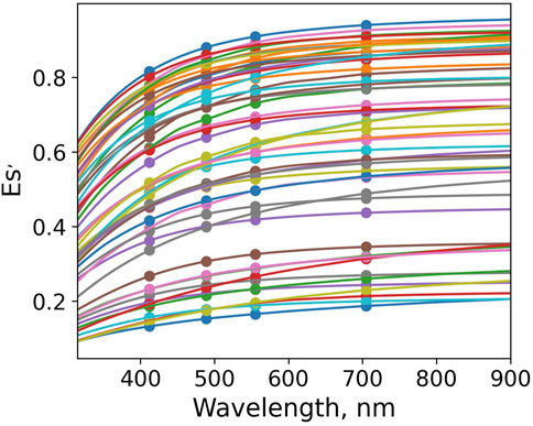
The hypothesis that it is feasible to reconstruct ${\mathit{E}}_{\mathit{s}}$ at hyper-spectral resolution using measurements at only a few bands is based on the fact that ${\mathit{E}}_{\mathit{s}}$ after the correction of gaseous absorption and normalization using the extraterrestrial solar irradiance, i.e., ${\mathit{E}}_{\mathit{s}}^{\prime }{=\mathit{E}}_{\mathit{s}}/\left({\mathit{E}}_{\mathbf{0}}{\mathit{T}}_{\mathit{g}}\right)$, essentially becomes ${\mathit{T}}_{\mathit{a}}\mathit{cos}\left({\mathit{\theta }}_{\mathit{s}}\right)/\left(\mathbf{1}-{\mathit{S}}_{\mathit{a}}\mathit{A}\right)$, which varies smoothly with wavelength (Figure 1). However, even though ${\mathit{E}}_{\mathit{s}}^{\prime }$ does not exhibit an irregular spectral dependence, its reconstruction via interpolation/extrapolation of measurements in a few bands may not be sufficiently accurate (see Section 4). Therefore, we tested two different models:

1. Multivariate linear model with constant coefficients (Eq. 2).

${\mathit{E}}_{\mathit{s}}^{\prime }\left(\mathit{\lambda }\right)={\mathit{a}}_{\mathbf{0}}+{\sum }_{\mathit{i}}{\mathit{a}}_{\mathit{i}}{\mathit{E}}_{\mathit{s}}^{\prime }\left({\mathit{\lambda }}_{\mathit{i}}\right)(2)$

where ${\mathit{a}}_{\mathbf{0}}$ is a constant, $\mathit{\lambda }$ represents wavelength, ${\mathit{E}}_{\mathit{s}}^{\prime }\left({\mathit{\lambda }}_{\mathit{i}}\right)$ and ${\mathit{a}}_{\mathit{i}}$ are the ${\mathit{E}}_{\mathit{s}}^{\prime }$ and the corresponding linear coefficients at ${\mathit{\lambda }}_{\mathit{i}}$, the center wavelengths $i$ of the 412, 489, 555, and 705 nm bands.

2. Generalized additive model (GAM; Hastie and Tibshirani, 1993) with coefficients as functions of geometric and/or geophysical parameters (Eq. 3).

${\mathit{E}}_{\mathit{s}}^{\prime }\left(\mathit{\lambda }\right)={\mathit{f}}_{\mathbf{0}}\left({\mathit{p}}_{\mathbf{1}},{\mathit{p}}_{\mathbf{2}},\dots ,{\mathit{p}}_{\mathit{n}}\right)+{\sum }_{\mathit{i}}{\mathit{f}}_{\mathit{i}}{\left({\mathit{p}}_{\mathbf{1}},{\mathit{p}}_{\mathbf{2}},\dots ,{\mathit{p}}_{\mathit{n}}\right)\mathit{E}}_{\mathit{s}}^{\prime }\left({\mathit{\lambda }}_{\mathit{i}}\right)(3)$

where ${\mathit{p}}_{\mathbf{1}},{\mathit{p}}_{\mathbf{2}},\dots ,{\mathit{p}}_{\mathit{n}}$ represent the various geometric and/or geophysical parameters to be used, and $\mathit{f}$ are functions of these variables. The parameters $\mathit{p}$ are selected based on analysis of the data. The $\mathit{f}$ functions constitute the free parameters of the model and will be estimated from the data. The shapes of $\mathit{f}$ are largely unspecified in the fitting procedure, while the resulting number of degrees of freedom are controlled to avoid overfitting. This is achieved via penalized smoothing splines.

FIGURE 1

FIGURE 1. Es’of the 50 cases simulated using ARTDECO with parameters randomly selected, i.e., different aerosol models (maritime clean, continental, urban, desert), aerosol optical thickness at 550 nm from 0 to 0.8, aerosol scale height from 0.5 to 5 km, relative humidity from 60% to 90%, ozone amount from 250 to 450 Dobson, water vapor from 0.1 to 7 g cm⁻², surface pressure from 1,000 to 1,025 mb, solar zenith angle from 0° to 75°, wind speed from 5 to 15 m s⁻¹, and chlorophyll concentration from 0.3 to 30 mg m⁻³. Dots represent the Es’ values at 412, 489, 555, and 705 nm.

Once ${\mathit{E}}_{\mathit{s}}^{\prime }$ is retrieved, ${\mathit{E}}_{\mathit{s}}$ can be derived from ${\mathit{E}}_{\mathit{s}}^{\prime }$ since ${\mathit{E}}_{\mathbf{0}}$ is known and ${\mathit{T}}_{\mathit{g}}$ can be accurately estimated (see Section 4). Uncertainties of the two methods are quantified by introducing noise to the input ${\mathit{E}}_{\mathit{s}}$ at the four wavelengths, together with assigning noise to ${\mathit{T}}_{\mathit{g}}$, which will then be propagated to estimate the uncertainties in reconstructed ${\mathit{E}}_{\mathit{s}}$ using the Monte-Carlo method (e.g., JCGM, 2008; Bialek et al., 2020. This requires the probability distribution functions for the input components in the model equation (content of gaseous absorbers in the multilinear model with constant coefficients and, additionally, the auxiliary variables in the additive varying coefficient model), from which many random realizations are selected in the calculation of the output, providing the uncertainty of the output value.

The reconstruction of ${\mathit{E}}_{\mathit{s}}$ described above is accomplished with respect to the extraterrestrial solar spectrum ${\mathit{E}}_{\mathbf{0}}$ used in the radiative transfer (RT) model. One has to be aware of this in calibration/validation activities and make sure that the same ${\mathit{E}}_{\mathbf{0}}$ is used. Using a different ${\mathit{E}}_{\mathbf{0}}$, however, does not require re-determining the coefficients of the ${\mathit{E}}_{\mathit{s}}^{\prime }$ model (Eq. 2).

3 Simulations

Radiative transfer simulations were performed from 315 to 900 nm at 0.5 nm resolution with the Atmospheric Radiative Transfer Database for Earth Climate Observation (ARTDECO) code (Dubuisson et al., 2016) for a variety of geometric and geophysical conditions. The ARTDECO radiative transfer model accounts for scattering and absorption by air molecules, aerosols, and cloud droplets, and interactions between scattering and absorption. The radiative transfer equation is solved using the discrete ordinate method. The atmosphere is assumed plane-parallel and positioned above a wavy air-sea interface. In the code, the high-resolution extraterrestrial solar spectrum is from Chance and Kurucz (2010), mean Earth-Sun distance is used, and gaseous absorption is accounted for by applying the correlated-k technique (Lacis and Oinas, 1991) with appropriate k-distribution coefficients. The optical properties of aerosols and clouds are selected from the Optical Properties of Aerosols and Clouds (OPAC) database (Hess et al., 1998). The vertical distribution of the scatterers and absorbers can be specified. The bidirectional reflectance of the wavy interface is modeled based on Fresnel equations and the Cox-Munk wind-dependent wave slope probability density distribution. The diffuse water reflectance (Case 1 waters only) is assumed Lambertian and modeled as a function of chlorophyll concentration according to Morel and Maritorena (2001). This model, limited to the visible, was extended to 300 nm using Hydrolight (Hedley and Mobley, 2019) inherent optical properties. The water body is considered black at wavelengths longer than 700 nm. This treatment is sufficient because the impact of photons leaving the water that are backscattered by the atmosphere to the surface is relatively small.

The total downwelling solar irradiance arriving at the ocean surface ${\mathit{E}}_{\mathit{s}}$ was simulated from 315 to 900 nm with a 0.5 nm resolution for a clear atmosphere (i.e., no clouds). The corresponding extraterrestrial solar irradiance ${\mathit{E}}_{\mathbf{0}}$ was also output in the simulations. In the code, the AFGL US standard atmosphere profile (Anderson et al., 1986) was used and adapted to the input concentrations of gases, i.e., ozone, water vapor, and oxygen. Note that by explicitly varying the oxygen amount the absorption from other gases including CH₄, CO₂, and N₂O was considered since the molar fraction of these gases are fixed with respect to oxygen in the ARTDECO code. Since absorption from NO₂ was not modeled in ARTDECO, transmittance of NO₂ was estimated based on Schneider et al. (1987) and applied to the simulated ${\mathit{E}}_{\mathit{s}}$. In this study, the following three different datasets were generated.

1. Dataset for calibrating the models for ${\mathit{E}}_{\mathit{s}}$ reconstruction, referred as the calibration dataset.

In this dataset, four different aerosol models from the OPAC database were considered, i.e., maritime clean, continental clean, urban, and desert, including both absorbing and non-absorbing aerosols. The computations were conducted for total aerosol optical thickness values (AOT550) ranging from 0 to 0.8 at 550 nm. The aerosol concentration was set to decrease with altitude according to an exponential law with a typical scale height (SH) from 0.5 to 5 km. The relative humidity (RH) in the atmosphere was set to randomly vary from 60% to 90%. The amount of ozone (U_o3) and water vapor (U_h2o) were from 250 to 450 Dobson and from 0.1 to 7 g cm⁻², respectively. The oxygen amount is defined using surface pressure (PS), which was varied from 1,000 to 1,025 mb. Simulations were carried out for Sun zenith angles (SZAs) ranging from 0° to 75° (view zenith and relative azimuth were fixed as 0° and 90°, since they do not affect ${\mathit{E}}_{\mathit{s}}$). The wind speed (U) was set to vary from 5 to 15 m s⁻¹. The optical properties of the diffuse boundary marine reflectance were specified for chlorophyll concentration (Chl) varying from 0.03 to 30 mg m⁻³. A total of 10,000 simulations were performed, with aerosol types, aerosol optical thickness, scale height, humidity, ozone, surface pressure, water vapor, Sun zenith angle, wind speed, chlorophyll concentration randomly varied in the ranges described above. For each simulation with gaseous absorption, the case of no gaseous absorption was also generated to obtain ${\mathit{E}}_{\mathit{s}\mathbf{0}}$, i.e., ${\mathit{E}}_{\mathit{s}}$ after correction of gaseous absorption (${\mathit{E}}_{\mathit{s}}={\mathit{E}}_{\mathit{s}\mathbf{0}}{\mathit{T}}_{\mathit{g}}$).

2. Dataset for developing the Look-Up Table (LUT) of ${\mathit{T}}_{\mathit{g}}$, referred as the LUT dataset.

In this dataset, the ranges of different geometric and geophysical parameters are the same as those in the calibration dataset. What is different is that the input amount of ozone, water vapor and oxygen as well as Sun zenith angles were set to be discrete values as below.

• SZA (degree): 0, 10, 20, 30, 40, 50, 60, 65, 70, and 75

• U_o3 (Dobson): 250, 300, 350, 400, 450

• U_h2o (g cm⁻²): 0.1, 0.2, 0.3, 0.4, 0.5, 0.6, 0.7, 0.8, 0.9, 1, 2, 3, 4, 5, 6, 7

• PS (mb): 1,000, 1,005, 1,010, 1,015, 1,020, 1,025

Both simulations with and without gaseous absorption were made. The aerosol properties and surface conditions have a small impact on ${\mathit{T}}_{\mathit{g}}$, except in strong water vapor absorption bands, where the coupling between aerosol scattering and water vapor absorption becomes effective, but such bands occur above 900 nm. Therefore these parameters were fixed for each simulation, i.e., AOT550 = 0.1, RH = 90%, SH = 2 km, maritime aerosol, U = 5 m/s, and Ch1 = 0.1 mg/m³. The LUT has four axes, i.e., Sun zenith angle, ozone and water vapor amounts, and pressure.

3. Dataset for validating the models for ${\mathit{E}}_{\mathit{s}}$ reconstruction, referred as the validation dataset.

Instead of using the four different OPAC aerosols, this dataset uses mixed aerosols, i.e., all aerosol species were mixed up for each simulation. The aerosol species include black carbon (OPAC urban), dust (OPAC Desert), organic carbon (OPAC continental), and sea salt (OPAC maritime). Global hourly MERRA-2 reanalysis data (Gelaro et al., 2017) for the entire year 2006 were acquired to extract the optical thickness corresponding to each aerosol species, which were then randomly selected (covering global ocean) and input to ARTDECO. Other parameters were set in the same predefined ranges as in the calibration dataset but with totally different values. There are 10,000 simulations with gaseous absorption and another 10,000 without gaseous absorption. Noise was also added to this dataset to evaluate the sensitivity of the models to noise, of which the details are described in Section 4.

For the calibration and validation datasets, the ${\mathit{E}}_{\mathit{s}}$ and ${\mathit{E}}_{\mathit{s}\mathbf{0}}$ simulations at 0.5 nm resolution were further processed into the values in the 412, 488, 555, and 705 nm bands by using the average within ±5 nm of the center wavelengths (the exact spectral response of the bands was unknown).

4 Theoretical results

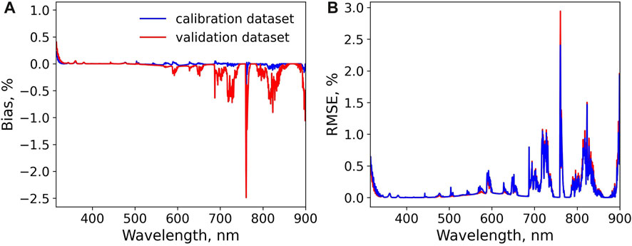
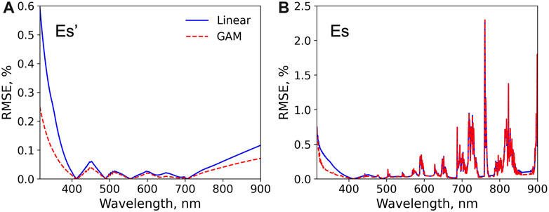
The LUT developed in Section 3 was used to estimate ${\mathit{T}}_{\mathit{g}}$ for the 10,000 cases in the calibration dataset and another 10,000 cases in the validation dataset using the prescribed solar zenith angle, ozone, amount, surface pressure, and water vapor amount as input and linearly interpolating within the LUT. Figure 2 shows that the LUT method produces accurate estimation of ${\mathit{T}}_{\mathit{g}}$, with the bias ranging from −0.6% to 0.3% and from −2.5% to 0.4% and RMS error (RMSE) within 2.5% and within 3%, for the calibration and validation dataset, respectively. The bias and RMSE for the calibration and validation dataset are different because the input parameters to the LUT are not exactly the same. Remember that −2.5% bias is equivalent a bias of −0.004, which is very small. As expected, degradation of accuracy is found at the wavelengths with gaseous absorption, for example, the ultra-violet (UV) and 500–700 nm with ozone absorption, ∼688 nm and ∼760 nm with strong oxygen absorption, and near-infrared with water vapor absorption, while at the wavelengths almost without gaseous absorption the bias and RMS error are close to 0. This is with the assumption that the amount of ozone, surface pressure, and water vapor are perfectly known. In practice, noise in these quantities will introduce uncertainties in the estimated ${\mathit{T}}_{\mathit{g}}$ and the impact on the ${\mathit{E}}_{\mathit{s}}$ reconstruction is investigated, as described in the text below.

FIGURE 2

FIGURE 2. Percent bias (A) and RMSE (B) of ${\mathit{T}}_{\mathit{g}}$ estimation using the calibration (blue) and validation (red) dataset.

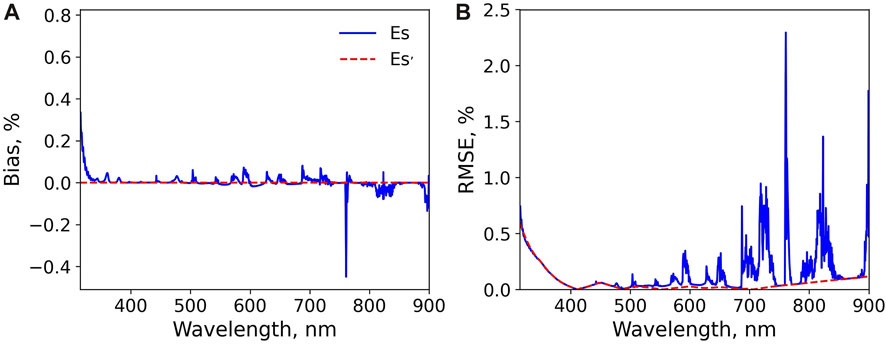
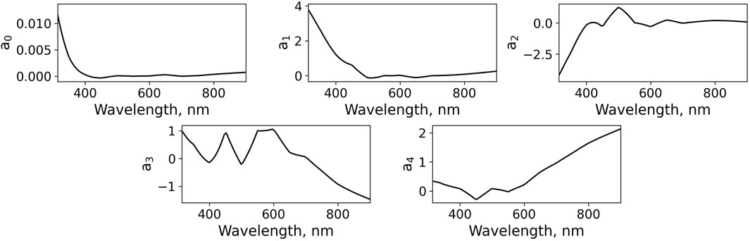
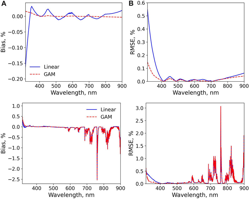
${\mathit{E}}_{\mathit{s}}^{\prime }$ at 0.5 nm resolution from 315 nm to 900 nm can be accurately reconstructed using the values at 412, 489, 555, and 705 nm using multivariate linear regression (Figure 3). The ${\mathit{a}}_{\mathbf{0}}$ and ${\mathit{a}}_{\mathit{i}}$ coefficients in Eq. 2, are irregular spectrally (Figure 4), an indication that simple interpolation/extrapolation would not capture spectral ${\mathit{E}}_{\mathit{s}}^{\prime }$ variability as well as the multilinear model. Bias is 0 for all the wavelengths, which is not surprising because the model is supposed to be unbiased. The RMSE is less than 0.1% starting from 400 nm and increases to 0.6% in the UV wavelengths. The relatively high error in the UV is probably due to the fact that the input four wavelengths are from 400 to 700 nm, which may fail to properly capture some of the spectral characteristics at the UV. The ${\mathit{E}}_{\mathit{s}}$ spectra were computed using ${\mathit{E}}_{\mathbf{0}}$ and the estimated ${\mathit{T}}_{\mathit{g}}$. The bias, ranging from −0.2% to 0.4%, and RMSE, from 0% to 2.5%, are basically the total of ${\mathit{T}}_{\mathit{g}}$ and ${\mathit{E}}_{\mathit{s}}^{\prime }$ errors, although some compensation occurs so that the values are slightly lower.

FIGURE 3

FIGURE 3. Percent bias (A) and RMSE (B) of ${\mathit{E}}_{\mathit{s}}^{\prime }$ (red dashed) and ${\mathit{E}}_{\mathit{s}}$ (blue solid) estimation using the calibration dataset and multivariate linear regression.

FIGURE 4

FIGURE 4. Coefficients of the multilinear model (see Eq. 2).

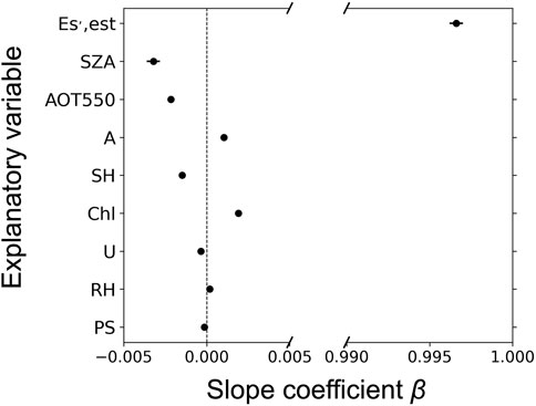
The prescribed ${\mathit{E}}_{\mathit{s}}^{\prime }$ was further modeled as a function of all other variables, including the estimated ${\mathit{E}}_{\mathit{s}}^{\prime }$ (${\mathit{E}}_{\mathit{s},\mathit{e}\mathit{s}\mathit{t}}^{\prime }$), SZA, AOT550, SH, aerosol model (A), Chl, U, RH, and PS, following the procedure of Bisson et al. (2021) using a Bayesian approach to multivariate regression analysis. U_o3 and U_h2o were not included because ${\mathit{E}}_{\mathit{s}}^{\prime }$ is the quantity after gaseous absorption. The regression model is assumed to follow a normal distribution with the mean $\mathit{\mu }$ modeled as in Eq. 4

$\mathit{\mu }={\mathit{\beta }}_{\mathbf{0}}{\mathit{E}}_{\mathit{s},\mathit{e}\mathit{s}\mathit{t}}^{\prime }+{\mathit{\beta }}_{\mathbf{1}}\mathit{S}\mathit{Z}\mathit{A}+{\mathit{\beta }}_{\mathbf{2}}\mathit{A}\mathit{O}\mathit{T}\mathbf{550}+{\mathit{\beta }}_{\mathbf{3}}\mathit{S}\mathit{H}+{\mathit{\beta }}_{\mathbf{4}}\mathit{A}+{\mathit{\beta }}_{\mathbf{5}}\mathit{C}\mathit{h}\mathit{l}+{\mathit{\beta }}_{\mathbf{6}}\mathit{U}+{\mathit{\beta }}_{\mathbf{7}}\mathit{R}\mathit{H}+{\mathit{\beta }}_{\mathbf{8}}\mathit{P}\mathit{S}+\mathit{\alpha }(4)$

Each variable was standardized by subtracting the mean and dividing by the standard deviation to shift the distribution to have a mean of zero and a standard deviation of one. By doing so, the intercept bias $\mathit{\alpha }$ essentially becomes zero and the slope coefficients ${\mathit{\beta }}_{\mathit{i}}$ illustrate a one-to-one correspondence between the dependent and independent variables. In the model, the prior distribution of ${\mathit{\beta }}_{\mathit{i}}$ is assumed weakly informative, with mean of zero and a standard deviation of 100. For example, at 320.25 nm, the slope coefficient ${\mathit{\beta }}_{\mathbf{0}}$ is very close to 1, i.e., ∼0.997 (Figure 5), indicating strong correspondence between ${\mathit{E}}_{\mathit{s}}^{\prime }$ and ${\mathit{E}}_{\mathit{s},\mathit{e}\mathit{s}\mathit{t}}^{\prime }$. The $\mathit{\beta }$ for other variables all deviate from 0, although the deviations are small, indicating their contribution to residual errors. Based on the magnitude of the $\mathit{\beta }$ values, the three variables with the highest absolute values are SZA, AOT550, and Chl. Large percent errors are typically found to be associated with small ${\mathit{E}}_{\mathit{s}}^{\prime }$, which is not easy to model accurately. When SZA is large, it means longer travelling path and more interactions of the light with aerosols and molecules in the atmosphere. The larger AOT550, the more aerosol scattering and absorption, depending on the aerosol types. Both variables lead to small ${\mathit{E}}_{\mathit{s}}^{\prime }$ and may explain their relatively large contributions in the residual errors. The variations in chlorophyll concentration affect the ocean surface albedo. In the UV, when chlorophyll concentration is small, the ocean surface albedo becomes relatively large and the spherical albedo of the atmosphere is increased, hence the surface impact introduced by the term $\mathbf{1}/\left(\mathbf{1}-{\mathit{S}}_{\mathit{a}}\mathit{A}\right)$ may cause perturbations in ${\mathit{E}}_{\mathit{s}}^{\prime }$ and inaccuracy in the modeling.

FIGURE 5

FIGURE 5. Forest plot of the slope coefficients for wavelength 320.25 nm. The y axis shows the coefficients β for each explanatory variable, i.e., estimated ${\mathit{E}}_{\mathit{s}}^{\prime }$ (${\mathit{E}}_{\mathit{s},\mathit{e}\mathit{s}\mathit{t}}^{\prime })$, solar zenith angle (SZA), aerosol optical thickness (AOT550), aerosol model (A), scale height (SH), chlorophyll concentration (Chl), wind speed (U), relative humidity (RH), and surface pressure (PS), and the x axis shows the scale of the coefficients. The circle presents the mean of the posterior and the error bar represents the standard deviation of the distribution.

The variables SZA, AOT550, aerosol type, SH, Chl, U, RH, and PS were then tested in the GAM model. These variables were introduced one by one and only those that brought in significant model improvement were selected, i.e., SZA and AOT550 in this study. The GAM model therefore becomes Eq. 5:

${\mathit{E}}_{\mathit{s}}^{\prime }\left(\mathit{\lambda }\right)={\mathit{f}}_{\mathbf{0}}\left(\mathit{S}\mathit{Z}\mathit{A},\mathit{A}\mathit{O}\mathit{T}\mathbf{550}\right)+{\sum }_{\mathit{i}}{\mathit{f}}_{\mathit{i}}{\left(\mathit{S}\mathit{Z}\mathit{A},\mathit{A}\mathit{O}\mathit{T}\mathbf{550}\right)\mathit{E}}_{\mathit{s}}^{\prime }\left({\mathit{\lambda }}_{\mathit{i}}\right)(5)$

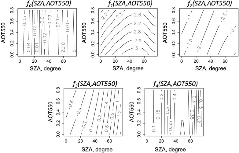
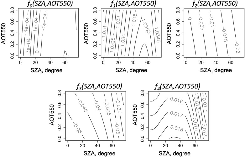
With the coefficients as a function of SZA and AOT550 instead of assumed constant, the accuracy of ${\mathit{E}}_{\mathit{s}}^{\prime }$ reconstruction is improved (Figure 6). The bias is not discussed here because both models are unbiased. The change of percent RMSE with wavelength shows a pattern similar to that obtained using multivariate linear regression, i.e., the closer the wavelength is to one of the input four bands the smaller the RMSE. Overall, the magnitude is lower for GAM as opposed to the linear model, especially in the wavelengths shorter than 400 nm and those longer than 700 nm. For example, the error drops from 0.6% to 0.2% in the UV and from 0.1% to 0.06% at 900 nm. An even stronger decrease of RMSE in the UV and from 850 to 900 nm is observed for the ${\mathit{E}}_{\mathit{s}}$ reconstruction when using GAM. The terms of the five components (i.e., the functions ${\mathit{f}}_{\mathbf{0}}$, ${\mathit{f}}_{\mathbf{1}}$, ${\mathit{f}}_{\mathbf{2}}$, ${\mathit{f}}_{\mathbf{3}}$ and ${\mathit{f}}_{\mathbf{4}}$) of the GAM model at 320.25 nm and 410.25 nm are displayed in Figures 7, 8, respectively. It is thus clear that the intercept as well as the coefficients for ${\mathit{E}}_{\mathit{s}}^{\prime }$ at the four wavelengths are not constant and the contours show how the values of ${\mathit{f}}_{\mathit{i}}$ change with SZA and AOT550. The gradients of the component smooth functions ${\mathit{f}}_{\mathit{i}}$ at 410.25 nm are much smaller than those at 310.25 nm, which is expected as the residual errors in ${\mathit{E}}_{\mathit{s}}^{\prime }$ attributed to SZA and AOT550 are more pronounced in the UV. At 320.25 nm the gradient of each ${\mathit{f}}_{\mathit{i}}$ changes with SZA, while the impact AOT550 is more obvious on ${\mathit{f}}_{\mathbf{1}}$, ${\mathit{f}}_{\mathbf{2}}$, and ${\mathit{f}}_{\mathbf{3}}$ and becomes less important for ${\mathit{f}}_{\mathbf{0}}$ and ${\mathit{f}}_{\mathbf{4}}$. This is the same with 410.25 nm, i.e., the changes in ${\mathit{f}}_{\mathit{i}}$ with respect to AOT550 decrease with wavelength, probably due to that aerosol scattering is stronger at shorter than longer wavelengths. Although the impact of AOT550 may be small and negligible depending on the smooth functions and the wavelength, AOT550 is kept in the GAM model so that we do not need to optimize the model for each wavelength, which is out of the scope of this study.

FIGURE 6

FIGURE 6. Percent RMSE of ${\mathit{E}}_{\mathit{s}}^{\prime }$ (A) and ${\mathit{E}}_{\mathit{s}}$ (B) estimation using the calibration dataset with both models: (blue) multivariate linear regression and (red) GAM. Percent bias is not shown as both models result in almost identical bias for ${\mathit{E}}_{\mathit{s}}^{\prime }$ and ${\mathit{E}}_{\mathit{s}}$.

FIGURE 7

FIGURE 7. The five component smooth functions (${\mathit{f}}_{\mathbf{0}}$, ${\mathit{f}}_{\mathbf{1}}$, ${\mathit{f}}_{\mathbf{2}}$, ${\mathit{f}}_{\mathbf{3}}$, and ${\mathit{f}}_{\mathbf{4}}$) of the GAM model fitted on the calibration data at 320.25 nm.

FIGURE 8

FIGURE 8. Same as Figure 7, but for 410.25 nm.

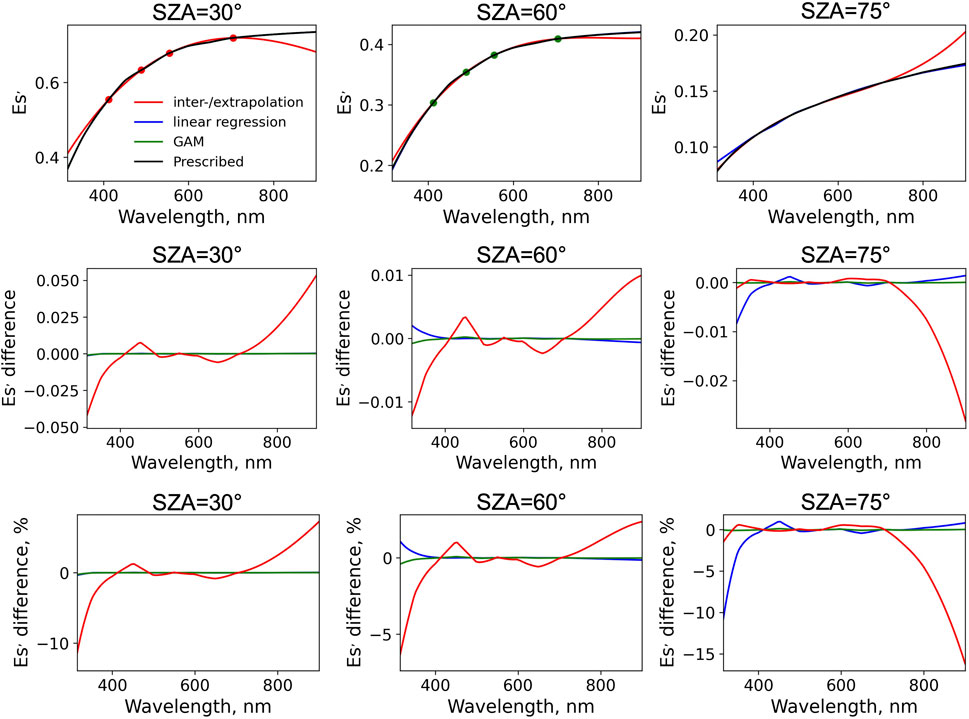
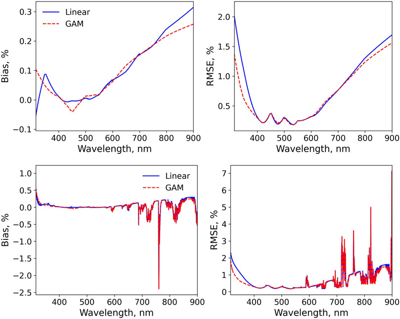
Performance of both models in reconstructing ${\mathit{E}}_{\mathit{s}}^{\prime }$ and ${\mathit{E}}_{\mathit{s}}$ with the validation dataset are very similar to those with the calibration dataset (Figure 9). For ${\mathit{E}}_{\mathit{s}}^{\prime }$ reconstruction, the percent bias is from −0.15% to 0.03% for the multivariate linear model and from −0.01% to 0.02% for the GAM model, and the precent RMSE from 0% to 0.55% and from 0% to 0.15%, respectively. The bias and RMSE of ${\mathit{E}}_{\mathit{s}}$ are higher than those with the calibration dataset (Figure 2), from −2.5% to −0.5% and from 0% to 3%, respectively, mainly attributed to the errors in ${\mathit{T}}_{\mathit{g}}$ estimation (Figure 2). Figure 10 shows that simply using interpolation/extrapolation to reconstruct the hyperspectral ${\mathit{E}}_{\mathit{s}}^{\prime }$ from only four values typically yield much larger errors when compared to the multivariate linear model and GAM, especially in the ultraviolet wavelengths and at high Sun zenith angles.

FIGURE 9

FIGURE 9. Percent bias and RMSE in the reconstructed of ${\mathit{E}}_{\mathit{s}}^{\prime }$ (A) and ${\mathit{E}}_{\mathit{s}}$ (B) using the multivariate linear model (blue) and GAM (red) with the validation data set.

FIGURE 10

FIGURE 10. Comparison of the reconstructed ${\mathit{E}}_{\mathit{s}}^{\prime }$ using interpolation/extrapolation, multivariate linear model, and GAM for three cases in the calibration dataset with solar zenith angle (SZA) of 30°, 60°, and 75°. ${\mathit{E}}_{\mathit{s}}^{\prime }$ difference is defined as the prescribed minus the reconstructed value.

In practice the in-situ measurements may be biased due to instrument calibration uncertainty and other uncertainties, (e.g., data processing). It is important to check the in-situ dataset against radiative transfer calculations before performing the spectral reconstruction, which can be accomplished by comparing measurements and modeled values in ideal conditions, i.e., very clear atmosphere with low aerosol content. Assuming such check has been performed and environmental uncertainty is negligible, the remaining noise, i.e., which defines the ${\mathit{E}}_{\mathit{s}}$ calibration uncertainty, is about ±1%, according to Bialek et al. (2020) for an ideal case with no bias.

This noise was added to ${\mathit{E}}_{\mathit{s}}$ in the validation dataset based on Eq.6 displayed below,

${\mathit{E}}_{\mathit{s},\mathit{n}\mathit{o}\mathit{i}\mathit{s}\mathit{y}}={\mathit{E}}_{\mathit{s}}\left(\mathbf{1}+\mathit{e}\right)(6)$

where $\mathit{e}$ is a gaussian distributed variable with standard deviation of 0.01. Note that there are other sources of uncertainty in the ${\mathit{E}}_{\mathit{s}}$, such as that caused by converting the 0.5 nm simulated ${\mathit{E}}_{\mathit{s}}$ to multispectral values, but here only the calibration error $\mathit{e}$ is considered. In addition, noise was added to U_o3, U_h2o, and PS, i.e., ±10 Dobson, ±20%, and ±5 mb, respectively, to account for the uncertainty in the MERRA-2 data. No uncertainty in ${\mathit{E}}_{\mathit{o}}$ and in the radiative transfer modeling was considered. The Monte Carlo approach described in JCGM (2008) was used to quantify the final uncertainties in the reconstructed ${\mathit{E}}_{\mathit{s}}$. A total of 100 hyperspectral ${\mathit{E}}_{\mathit{s}}$ were reconstructed with random realizations of noise specified above and the bias and RMSE were calculated against the prescribed values.

When using the multivariate linear model on the noisy data, the percent bias and RMSE in ${\mathit{E}}_{\mathit{s}}^{\prime }$ could reach 0.3% and about 2.0%, respectively (Figure 11), which generally increase in the UV and near infrared and decrease (i.e., less than 0.1% and 0.5%, respectively) in the visible. The errors in ${\mathit{E}}_{\mathit{s}}$ are larger, with the largest bias and RMSE being −2.5% and 7.0% respectively. Relatively large errors are typically found in the spectral region of the gaseous absorption bands and at UV wavelengths. The GAM model produces very similar level of bias and RMSE in the ${\mathit{E}}_{\mathit{s}}^{\prime }$ estimation. Considering that the GAM model is more accurate than the multivariate linear model, especially in the UV, as well as that the uncertainty of GAM estimated ${\mathit{E}}_{\mathit{s}}^{\prime }$ was calculated assuming AOT550 is perfectly known, the results suggest that the GAM model is slightly more sensitive to noise, as the bias and RMSE between the two models become closer after introducing noise. In fact, the bias and RMSE for ${\mathit{E}}_{\mathit{s}}$ are very similar for both models and much larger than those for ${\mathit{E}}_{\mathit{s}}^{\prime }$, indicating the large impact from the noise in ${\mathit{T}}_{\mathit{g}}$.

FIGURE 11

FIGURE 11. Same as Figure 9, but with noise added to ${\mathit{E}}_{\mathit{s}}$ in the validation dataset and typical noise added to U_h2o, U_o3, and PS in ${\mathit{T}}_{\mathit{g}}$ estimation. See text for more details.

5 Evaluation against in situ measurements

The performance of ${\mathit{E}}_{\mathit{s}}$ reconstruction when applied to in-situ measurements was evaluated. Only the multivariate linear model was used since it is sufficiently accurate and slightly less sensitive to noise. In this study, two different in-situ datasets were used. The first one is the MOBY dataset, which has been collected off Lanai, Hawaii since 1997 (Clark et al., 1997; Clark et al., 2002) and used for vicarious calibration of many NASA, NOAA, and international satellite programs. MOBY is a spar buoy tethered to a slack-line moored buoy and has 3 underwater arms fixed at approximately 1, 5, and 9 m to take measurements of upwelling radiance and downwelling irradiance. Above-water downwelling irradiance is also measured using the ${\mathit{E}}_{\mathit{s}}$ sensor mounted on top of the buoy, which is about 2.5 m above the surface float. For more details see Clark et al., 1997; Clark et al., 2002. The MOBY ${\mathit{E}}_{\mathit{s}}$ data is hyperspectral and sampled every 0.8 nm from 344 nm to 750 nm, with the spectral resolution of approximately 0.9 nm for the blue (<620 nm) and 1.2 nm for the red (>620 nm). The data is publicly available at https://www.star.nesdis.noaa.gov/socd/moby/filtered_spec/. October 2016 reprocessing was applied. Note that the ${\mathit{E}}_{\mathit{s}}$ data below 380 nm is affected by stray light in the spectrometer (Feinholz et al., 2009). Only the data flagged as good were used in this study and there are a total of 7,036 data files available. In each data file, three columns of ${\mathit{E}}_{\mathit{s}}$ are provided, to match the measurements taken at the three underwater arms. The three ${\mathit{E}}_{\mathit{s}}$ values are very similar since they were taken in a short time period and only ${\mathit{E}}_{\mathit{s}}$ corresponding to the times of measurements by the middle arm were used. These MOBY data were checked against ARTDECO simulations made using MERRA-2 data corresponding to the MOBY observation time and a minor wavelength shift, i.e., 0.3 nm toward short wavelengths, was noticed. Since the MOBY data are very close to the ARTDECO simulations (i.e., within uncertainties in the modeling), no bias adjustment was made, but the wavelength shift was corrected for each measurement.

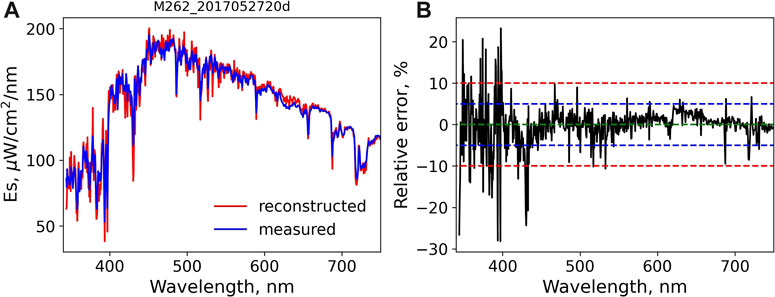
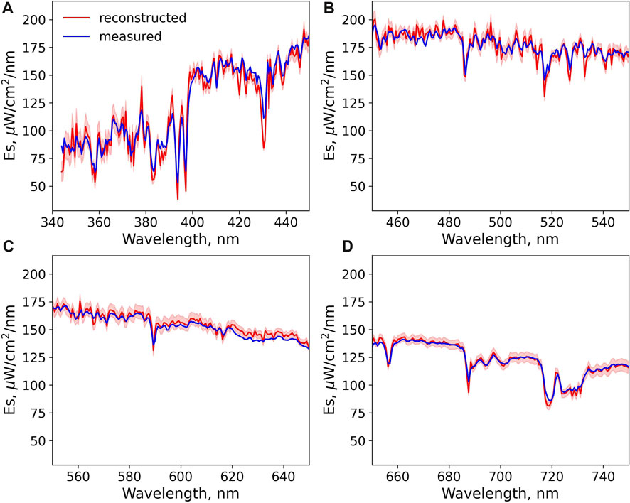
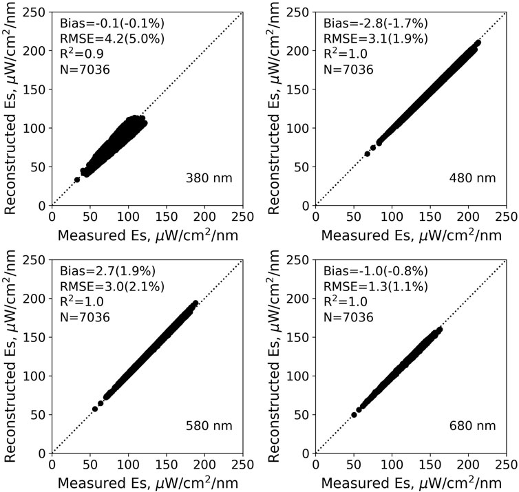
Figure 12 displays one example of the reconstructed MOBY ${\mathit{E}}_{\mathit{s}}$ on 27 May 2017. The measured and reconstructed ${\mathit{E}}_{\mathit{s}}$ are in very good agreement with the relative percent difference mostly within 10% over the entire wavelength range and less than 5% above 450 nm. The reconstruction at the UV wavelengths is noisier, attributed to the model noise and the stray light issue of the MOBY ${\mathit{E}}_{\mathit{s}}$ sensor. The relative error is also higher in the gaseous absorption bands. Uncertainties of the reconstructed ${\mathit{E}}_{\mathit{s}}$ were calculated by introducing the typical uncertainties in MOBY ${\mathit{E}}_{\mathit{s}}$, i.e., approximately ±1.5% for the laboratory and ±3.0% for the field (Voss et al., 2015), ±10 Dobson for U_o3, ±20% for U_h2o, ±5 mb for PS, as well as the model noise shown in Figure 3 (blue line, right panel). After that, 100 random realizations were generated, and the final uncertainty, i.e., the standard deviation of ${\mathit{E}}_{\mathit{s}}$ with noise, was calculated using all realizations. The measured values are generally within the uncertainties of the reconstructed ${\mathit{E}}_{\mathit{s}}$ (Figure 13). For all the 7,036 cases, the reconstructed ${\mathit{E}}_{\mathit{s}}$ are in very good agreement with the measured values, with the bias less than 2% and RMSE less than 5% (Figure 14). The bias and RMSE at wavelengths affected by gaseous absorption are larger. For example, at 688 nm and 720 nm, corresponding to oxygen and water vapor absorption, the corresponding bias and RMSE are 2.2% and 3.6%, and −4.2% and 6.3%, respectively. Such uncertainties are higher than those obtained using the theoretical data (Figure 11, bottom panel), which may be due to noise that are not accounted for when evaluating the model performance using the theoretical data.

FIGURE 12

FIGURE 12. (A) Measured and reconstructed MOBY ${\mathit{E}}_{\mathit{s}}$ on 27 May 2017, and (B) percent relative error between the measured and reconstructed ${\mathit{E}}_{\mathit{s}}$. Green, blue, and red dashed lines correspond to 0, 5, and 10% errors, respectively.

FIGURE 13

FIGURE 13. Comparisons between measured and reconstructed MOBY ${\mathit{E}}_{\mathit{s}}$ on 27 May 2017 at (A) 340–450 nm, (B) 450–550 nm, (C) 550–650 nm, and (D) 650–750 nm. Shaded areas indicate the uncertainties of the reconstructed ${\mathit{E}}_{\mathit{s}}$.

FIGURE 14

FIGURE 14. Comparisons between measured and reconstructed MOBY ${\mathit{E}}_{\mathit{s}}$ at 380, 480, 580, and 680 nm.

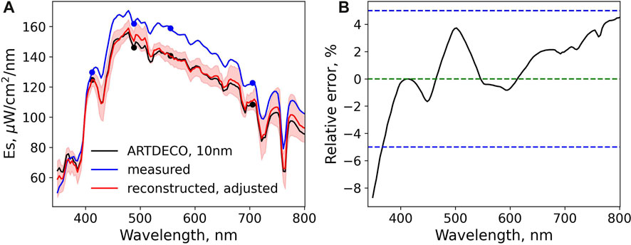
The second ${\mathit{E}}_{\mathit{s}}$ dataset used for evaluation was acquired with a Sea-Bird Scientific HyperOCR radiometer from June 10 to 16 June 2021 within sight of the MOBY buoy in Hawaii (20° 49′ 54.582″ N, 157° 11′ 19.062″ W). The measurements were made from the top of a 30 feet fishing vessel with an unobstructed view of the sky between 10:00 and 14:00 local time. The HyperOCR radiometer was calibrated by Sea-Bird Scientific with an FEL lamp pre and post deployment. The HyperOCR ${\mathit{E}}_{\mathit{s}}$ ranges from 349 to 801 nm and is sampled every 3 nm, with a spectral resolution of 10 nm. Only the data collected during clear sky conditions were used, which resulted in only one measurement on 16 June 2021. A check with ARTDECO code corresponding to the field observation time and conditions (obtained from MERRA-2 data) suggested that the HyperOCR ${\mathit{E}}_{\mathit{s}}$ values are biased, with the difference up to about 20 μW/cm²/nm (Figure 15). After adjusting the ${\mathit{E}}_{\mathit{s}}$ at the four wavelengths to the simulated values, the reconstruction was performed, with the uncertainties quantified in the same way as for the MOBY data. The measured values are mostly outside the uncertainty of the reconstructed ${\mathit{E}}_{\mathit{s}}$, confirming the possible bias existing in the measurements. The relative errors between the reconstructed and simulated ${\mathit{E}}_{\mathit{s}}$ using the 4 spectral bands are within 5% from 380 to 800 nm and go up to ∼9% at 350 nm. It is within expectation that the relative differences between the reconstructed and measured 10-nm resolved HyperOCR ${\mathit{E}}_{\mathit{s}}$ are lower than those with MOBY data, which has approximately 1 nm resolution.

FIGURE 15

FIGURE 15. (A) Measured (blue solid) HyperOCR ${\mathit{E}}_{\mathit{s}}$ on 16 June 2021. ATDECO simulations (black solid) show that the HyperOCR ${\mathit{E}}_{\mathit{s}}$ is off and needs to be adjusted. The reconstructed ${\mathit{E}}_{\mathit{s}}$ after adjustment (red solid) shows good agreement with the ARTDECO simulated values. Shaded areas indicate the uncertainties of the reconstructed ${\mathit{E}}_{\mathit{s}}$. (B) Percent relative error between the ARTDECO simulated and the reconstructed ${\mathit{E}}_{\mathit{s}}$ after adjustment. Green and blue dashed lines correspond to 0% and 5% errors, respectively. Blue and black dots represent the ${\mathit{E}}_{\mathit{s}}$ measured before and after adjustment.

6 Discussion

As demonstrated in the previous sections, both the multivariate linear and GAM models are capable of accurately reconstructing ${\mathit{E}}_{\mathit{s}}$ at 0.5 nm from four 10 nm wide spectral bands centered on 412, 489, 555, and 705 nm. The multivariate linear model is straightforward, easy to interpret, and well suited for the problem in this study, i.e., ${\mathit{E}}_{\mathit{s}}$, after normalization of the incoming TOA solar irradiance and correction of gaseous absorption, exhibits a smooth wavelength-dependent behavior. Conversely, the GAM model is more sophisticated and has advantages in complex nonlinear relationships. By varying the coefficients as functions of SZA and AOT550 in the GAM, the accuracy in reconstructing ${\mathit{E}}_{\mathit{s}}$ is slightly improved. This is consistent with the analysis of the correspondence between ${\mathit{E}}_{\mathit{s}}^{\prime }$ and different variables (Figure 5). This analysis suggests that only small residual errors exist between the ${\mathit{E}}_{\mathit{s}}^{\prime }$ and ${\mathit{E}}_{\mathit{s},\mathit{e}\mathit{s}\mathit{t}}^{\prime }$, which indicates that the relation between the ${\mathit{E}}_{\mathit{s}}^{\prime }$ to be reconstructed and the ${\mathit{E}}_{\mathit{s}}^{\prime }$ at the four 10-nm bands is almost linear, and such residual errors can be explained by parameters including SZA and AOT550, the two parameters with the highest $\mathit{\beta }$ compared to other geophysical parameters. Moreover, it is worth noting that the GAM model is more sensitive to noise. As a result, it is concluded that multivariate linear model is a more suitable choice in this study in terms of model accuracy and sensitivity.

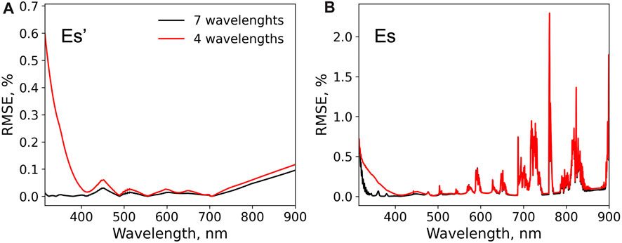
Instead of just utilizing the four multi-spectral bands at 412, 489, 555, and 705 nm, it is also possible to use other sets of wavelengths. For example, if we incorporate three additional wavelengths at UV, i.e., 325, 340, and 380 nm, the optional wavelengths that can be customized to the commercial Sea-Bird, Inc. OCR multi-spectral (7-band) radiometer, the RMSE of ${\mathit{E}}_{\mathit{s}}^{\prime }$ at UV exhibits significant reduction, with the maximum dropped from 0.6% to 0.02% and mostly remaining below 0.01% (Figure 16). The errors at other wavelengths also decrease to a certain extent, but not as much as in the UV. One may also be tempted to add more bands in the near infrared so that the RMSE can be further reduced in this range. However, one needs to have in mind that the major uncertainty comes from the estimation of ${\mathit{T}}_{\mathit{g}}$.

FIGURE 16

FIGURE 16. Percent RMSE of ${\mathit{E}}_{\mathit{s}}^{\prime }$ (A) and ${\mathit{E}}_{\mathit{s}}$ (B) estimation using multivariate linear regression with three extra wavelengths in the UV, i.e., 325, 340, and 380 nm (black), in comparison to original four input wavelengths (red) as shown in Figure 6. The regression was performed using the calibration dataset without noise.

In the evaluation of the model sensitivity to noise, it is found that the instrument calibration noise is the major contributor to the uncertainties in ${\mathit{E}}_{\mathit{s}}^{\prime }$. For example, at 320.25 nm, with no noise the percent bias and RMSE in ${\mathit{E}}_{\mathit{s}}^{\prime }$ are −0.01% and 0.50%, respectively; the percent RMSE increases to 1.82% if added noise and the percent bias remains the same. The noise in the input PS, U_o3, and U_h2o affect the estimation of ${\mathit{T}}_{\mathit{g}}$, and this is another important source of uncertainties in the final restitution of ${\mathit{E}}_{\mathit{s}}$, especially at wavelengths affected by gaseous absorption. When ${\mathit{T}}_{\mathit{g}}$ noise is included, the percent RMS of ${\mathit{E}}_{\mathit{s}}$ increases from 1.86% to 1.94% at 320.25 nm, but changes from 2.78% to 3.60% in the oxygen band near 760 nm. To ensure accurate ${\mathit{E}}_{\mathit{s}}$ reconstruction, it should be verified that the input multispectral ${\mathit{E}}_{\mathit{s}}$ is not biased, for example by checking against radiative transfer simulations during very clear sky conditions (i.e., with small aerosol content), as indicated in Section 2. If the input ${\mathit{E}}_{\mathit{s}}$ is biased, one may expect that the reconstructed ${\mathit{E}}_{\mathit{s}}$ will be biased and the uncertainties could be large.

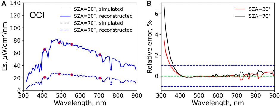
Since the presented method is capable of accurately reconstructing ${\mathit{E}}_{\mathit{s}}$ at 0.5 nm resolution, it can be easily adapted to different sensors with varying spectral characteristics. One potential and important use in the context of the upcoming PACE mission (scheduled to launched in February 2024) is reconstructing the OCI hyper-spectral ${\mathit{E}}_{\mathit{s}}$ signal using measurements in the four multi-spectral measurements of the current HyperNav system. Figure 17 illustrates an example of reconstructed ${\mathit{E}}_{\mathit{s}}$ at OCI wavelengths using simulated HyperNav ${\mathit{E}}_{\mathit{s}}$ measurements for a clear day. Results show that the OCI ${\mathit{E}}_{\mathit{s}}$ can be reconstructed accurately, with the relative differences within 1% from 360 nm to 900 nm. In the UV, the errors increase with wavelength, with the highest values of ∼4% and ∼7%, depending on the Sun zenith angle (high Sun zenith angle means low ${\mathit{E}}_{\mathit{s}}$ and relatively large uncertainties). With such reconstructed ${\mathit{E}}_{\mathit{s}}$ data, the HyperNav system is able to provide hyper-spectral ${\mathit{R}}_{\mathit{r}\mathit{s}}$ by normalizing the measured hyper-spectral ${\mathit{L}}_{\mathit{w}}$ against ${\mathit{E}}_{\mathit{s}}$, which has great significance for the calibration and validation of the PACE mission.

FIGURE 17

FIGURE 17. (A) The simulated (black) and reconstructed (blue) ${\mathit{E}}_{\mathit{s}}$ at PACE OCI wavelengths. The simulations are for a clear day with U_o3 = 300 Dobson, U_h2o = 2 g/cm², PS = 1,015 mb, Chl = 0.1 mg m⁻³, AOT550 = 0.1, maritime aerosol, relative humidity of 70%, SH = 2 km, and wind speed of 5 m s⁻¹. Two different SZA were used, i.e., 30° and 70°. The reconstruction was done using the simulated HyperNav values at the four wavelengths (red dots), i.e., 412, 489, 555, and 705 nm. (B) Percent relative error between the simulated and the reconstructed ${\mathit{E}}_{\mathit{s}}$. Green and blue dashed lines correspond to 0% and 1% errors, respectively. No noise has been added to the model input parameters.

7 Summary and conclusion

Spectral ${\mathit{E}}_{\mathit{s}}$ at 0.5 nm resolution can be reconstructed accurately from ${\mathit{E}}_{\mathit{s}}$ measurements in 4 spectral bands 10 nm-wide centered on 412, 489, 555, and 705 nm, such as those by an OCR SeaBird, Inc. planar irradiance sensor mounted on the HyperNav spectroradiometer/float system, using a multivariate linear model with constant coefficients or a GAM with coefficients dependent on SZA and AOT550. The models require as input, in addition to the 4 ${\mathit{E}}_{\mathit{s}}$ measurements, the content of gaseous absorbers (vertically integrated content for ozone and water vapor and surface pressure for oxygen and other gases). In the absence of noise, both models yield biases less than 0.4% in magnitude and RMSEs less than 2.5%. The largest errors are obtained in regions of strong absorption bands. Errors are smaller in the UV with the GAM model, i.e., 0.2% instead of 0.6%. In the presence of typical noise on the input variables, biases and RMSEs are generally less than 1.5% in magnitude and 3.5%, respectively, except in the center of the oxygen A-band (−2.7% and 5.3%). The GAM model is more sensitive to noise, i.e., the gain in accuracy in the UV in the absence of noise is practically lost in the presence of noise. The complexity of the GAM model, therefore, may not be justified, unless the typical noise in the input variables can be reduced. Using additional bands in the UV, i.e., at 325, 340, and 380 improves theoretical performance in the UV without noise, but marginally in practice because the ${\mathit{E}}_{\mathit{s}}$ error is dominated by ${\mathit{T}}_{\mathit{g}}$ uncertainties.

Evaluation of the multivariate linear model with constant coefficients against in-situ hyper-spectral ${\mathit{E}}_{\mathit{s}}$ measurements at the MOBY site revealed ${\mathit{E}}_{\mathit{s}}$ spectra reconstructed with biases less than 2% in magnitude and RMSE ranging from 1% to 2% in the visible to 5% in the UV, in agreement with theoretical uncertainties estimated using the Monte Carlo method. It is important, however, before doing any reconstruction, to check whether the multi-band E_s measurements are not biased (e.g., due to exposure, calibration, or processing errors), which can be accomplished by comparing the measurements to accurate radiative transfer calculations under favorable conditions. This revealed a significant bias in the HyperOCR ${\mathit{E}}_{\mathit{s}}$ data acquired near the MOBY site.

The methodology, by providing a way to accurately reconstruct ${\mathit{E}}_{\mathit{s}}$ at 0.5 nm resolution from ${\mathit{E}}_{\mathit{s}}$ measurements at a few 10 nm-wide spectral bands, as demonstrated theoretically and experimentally, allows normalization of hyper-spectral ${\mathit{L}}_{\mathit{w}}$ data acquired by HyperNav systems for validation activities of the PACE mission. The modeling does not replace hyper-spectral ${\mathit{E}}_{\mathit{s}}$ measurements, such as those made by the MOBY system, but is adequate in many aquatic optics applications, for which the acquisition of a relatively expensive hyper-spectral ${\mathit{E}}_{\mathit{s}}$ sensor, costly to maintain and calibrate, may therefore not be necessary. The methodology is applicable to other sets of spectral bands, i.e., those of other multi-band radiometers than the Seabird Inc. OCR used here, but accuracy of the reconstruction will depend on the bands position in the solar spectral range. Now, because the optical properties of clouds, like those of aerosols, and their effects on ${\mathit{E}}_{\mathit{s}}$ vary relatively smoothly with wavelength in the UV to near infrared, the modeling can be extended to estimating spectral ${\mathit{E}}_{\mathit{s}}$ in all sky conditions, although the coupling between absorption by gases and scattering by cloud droplets may complicate the treatment of ${\mathit{T}}_{\mathit{g}}$ in some spectral regions. Such extension is envisioned in future work.

Data availability statement

The original contributions presented in the study are included in the article, further inquiries can be directed to the corresponding author. The code for reconstructing from E_s measurements at 412, 489, 555, and 705 nm is publicly available at https://github.com/jit079/Es_reconstruction.

Author contributions

JT: Conceptualization, Investigation, Methodology, Writing–original draft, Writing–review and editing. RF: Conceptualization, Investigation, Methodology, Supervision, Writing–review and editing. NH: Writing–review and editing. AB: Writing–review and editing. EB: Writing–review and editing. PC: Writing–review and editing. MM: Writing–review and editing. CO: Writing–review and editing.

Funding

The author(s) declare that financial support was received for the research, authorship, and/or publication of this article. This work was supported by the National Aeronautics and Space Administration NASA under Grant 80GFC22CA050.

Acknowledgments

The authors gratefully acknowledge the MOBY team for generating, maintaining, and distributing the MOBY data used in this study, and the HyperNav engineers and technicians at SeaBird, Inc. for their help with HyperNav operations.

Conflict of interest

Author CO was employed by Sea-Bird Scientific.

The remaining authors declare that the research was conducted in the absence of any commercial or financial relationships that could be construed as a potential conflict of interest.

The author(s) declared that they were an editorial board member of Frontiers, at the time of submission. This had no impact on the peer review process and the final decision.

Publisher’s note

All claims expressed in this article are solely those of the authors and do not necessarily represent those of their affiliated organizations, or those of the publisher, the editors and the reviewers. Any product that may be evaluated in this article, or claim that may be made by its manufacturer, is not guaranteed or endorsed by the publisher.

References

Anderson, G. P., Clough, S. A., Kneizys, F. X., Chetwynd, J. H., and Shettle, E. P. (1986). AFGL atmospheric constituent profiles (0-120 km). Environ. Res. Pap., 954.

Google Scholar

Barnard, A., Boss, E., Haëntjens, N., Orrico, C., Frouin, R., Klumpp, J., et al. (2024). Design, characterization, and verification of a highly accurate in situ hyperspectral radiometric measurement system (HyperNAV). Submitted to Frontiers in Remote Sensing.

Google Scholar

Białek, A., Douglas, S., Kuusk, J., Ansko, I., Vabson, V., Vendt, R., et al. (2020). Example of Monte Carlo method uncertainty evaluation for above-water ocean colour radiometry. Remote Sens. 12, 780. doi:10.3390/rs12050780

CrossRef Full Text | Google Scholar

Bisson, K. M., Boss, E., Werdell, P. J., Ibrahim, A., Frouin, R., and Behrenfeld, M. J. (2021). Seasonal bias in global ocean color observations. Appl. Opt. AO 60, 6978–6988. doi:10.1364/AO.426137

CrossRef Full Text | Google Scholar

Chance, K., and Kurucz, R. L. (2010). An improved high-resolution solar reference spectrum for earth’s atmosphere measurements in the ultraviolet, visible, and near infrared. J. Quantitative Spectrosc. Radiatve Transf. 111, 1289–1295. doi:10.1016/j.jqsrt.2010.01.036

CrossRef Full Text | Google Scholar

Clark, D. K., Gordon, H. R., Voss, K. J., Ge, Y., Broenkow, W., and Trees, C. (1997). Validation of atmospheric correction over the oceans. J. Geophys. Res. Atmos. 102, 17209–17217. doi:10.1029/96JD03345

CrossRef Full Text | Google Scholar

Clark, D. K., Yarbrough, M. A., Feinholz, M. E., Flora, S., Broenkow, W., Johnson, B. C., et al. (2002). “MOBY, a radiometric buoy for performance monitoring and vicarious calibration of satellite ocean color sensors: measurement and data analysis protocols,” in Ocean optics protocols for satellite Ocean color sensor validation, revision 3. Greenbelt, MD, NASA goddard Space flight center. Editors J. L. Mueller,, and G. S. Fargion, 2. NASA/TM--2002-21004:138-170.

Google Scholar

Dubuisson, P., Labonnote, L. C., Riedi, J., Compiegne, M., and Winiarek, V. (2016). “ARTDECO: atmospheric radiative transfer database for earth and climate observation,” in International Radiation Symposium 2016, Auckland, New Zealand, April 2016, 17–22.

Google Scholar

Evans, R. H., and Gordon, H. R. (1994). Coastal zone color scanner “system calibration”: a retrospective examination. J. Geophys. Res. Oceans 99, 7293–7307. doi:10.1029/93JC02151

CrossRef Full Text | Google Scholar

Feinholz, M. E., Flora, S. J., Yarbrough, M. A., Lykke, K. R., Brown, S. W., Johnson, B. C., et al. (2009). Stray light correction of the marine optical system. J. Atmos. Ocean. Technol. 26, 57–73. doi:10.1175/2008JTECHO597.1

CrossRef Full Text | Google Scholar

Franz, B. A., Bailey, S. W., Werdell, P. J., and McClain, C. R. (2007). Sensor-independent approach to the vicarious calibration of satellite ocean color radiometry. Appl. Opt. AO 46, 5068–5082. doi:10.1364/AO.46.005068

PubMed Abstract | CrossRef Full Text | Google Scholar

Frouin, R. J., Franz, B. A., Ibrahim, A., Knobelspiesse, K., Ahmad, Z., Cairns, B., et al. (2019). Atmospheric correction of satellite ocean-color imagery during the PACE era. Front. Earth Sci. 7, 00145. doi:10.3389/feart.2019.00145

PubMed Abstract | CrossRef Full Text | Google Scholar

Gelaro, R., McCarty, W., Suárez, M. J., Todling, R., Molod, A., Takacs, L., et al. (2017). The modern-era retrospective analysis for research and applications, version 2 (MERRA-2). J. Clim. 30, 5419–5454. doi:10.1175/JCLI-D-16-0758.1

CrossRef Full Text | Google Scholar

Gordon, H. R. (1997). Atmospheric correction of ocean color imagery in the Earth Observing System era. J. Geophys. Res. Atmos. 102, 17081–17106. doi:10.1029/96JD02443

CrossRef Full Text | Google Scholar

Hastie, T., and Tibshirani, R. (1993). Varying-coefficient models. J. R. Stat. Soc. Ser. B Methodol. 55, 757–779. doi:10.1111/j.2517-6161.1993.tb01939.x

CrossRef Full Text | Google Scholar

Hedley, J. D., and Mobley, C. (2019). HydroLight 6.0 - EcoLight 6. 0 Users’ Guide Numerical Optics Ltd.

Google Scholar

Hess, M., Koepke, P., and Schult, I. (1998). Optical properties of aerosols and clouds: the software package OPAC. Bull. Am. Meteorological Soc. 79, 831–844. doi:10.1175/1520-0477(1998)079<0831:OPOAAC>2.0.CO;2

CrossRef Full Text | Google Scholar

IOCCG (2008). “Why ocean colour? The scocietal benefits of ocean-colour technology,” in Report No. 7 of the international ocean-colour coordinating group. Editors T. Platt, N. Hoepffner, V. Stuart, and C. Brown, Dartmouth, Canada: (Dartmouth: NS: IOCCG), 141.

Google Scholar

IOCCG (2013). “In-flight calibration of satellite ocean-colour sensors,” in Report No. 14 of the international ocean-colour coordinating group. Editor R. Frouin, Dartmouth, Canada: (Dartmouth, NS: IOCCG), 106.

Google Scholar

JCGM (2008). Evaluation of measurement data – supplement 1 to the “Guide to the expression of uncertainty in measurement” – propagation of distributions using a Monte Carlo method. Guidance Document. Avaialable at: https://www.bipm.org/documents/20126/2071204/JCGM_101_2008_E.pdf/325dcaad-c15a-407c-1105-8b7f322d651c.

Google Scholar

Lacis, A. A., and Oinas, V. (1991). A description of the correlated k distribution method for modeling nongray gaseous absorption, thermal emission, and multiple scattering in vertically inhomogeneous atmospheres. J. Geophys. Res. Atmos. 96, 9027–9063. doi:10.1029/90JD01945

CrossRef Full Text | Google Scholar

Morel, A., and Maritorena, S. (2001). Bio-optical properties of oceanic waters: a reappraisal. J. Geophys. Res. Oceans 106, 7163–7180. doi:10.1029/2000JC000319

CrossRef Full Text | Google Scholar

Mueller, J. L., Davis, C., Arnone, R., Frouin, R., Carder, K., Lee, Z. P., et al. (2003). “Above-water radiance and remote sensing reflectance measurements and analysis protocols,” in Ocean optics protocols for satellite Ocean color sensor validation revision 4; national aeronautical and Space administration (MD, USA: Greenbelt), III, 21–31. Chapter 3.

Google Scholar

Ruddick, K. G., Voss, K., Banks, A. C., Boss, E., Castagna, A., Frouin, R., et al. (2019a). A review of protocols for fiducial reference measurements of downwelling irradiance for the validation of satellite remote sensing data over water. Remote Sens. 11, 1742. doi:10.3390/rs11151742

CrossRef Full Text | Google Scholar

Ruddick, K. G., Voss, K., Boss, E., Castagna, A., Frouin, R., Gilerson, A., et al. (2019b). A review of protocols for fiducial reference measurements of water-leaving radiance for validation of satellite remote-sensing data over water. Remote Sens. 11, 2198. doi:10.3390/rs11192198

CrossRef Full Text | Google Scholar

Schneider, W., Moortgat, G. K., Tyndall, G. S., and Burrows, J. P. (1987). Absorption cross-sections of NO2 in the UV and visible region (200 – 700 nm) at 298 K. J. Photochem. Photobiol. A Chem. 40, 195–217. doi:10.1016/1010-6030(87)85001-3

CrossRef Full Text | Google Scholar

Tanré, D., Herman, M., Deschamps, P. Y., and Leffe, A. de (1979). Atmospheric modeling for space measurements of ground reflectances, including bidirectional properties. Appl. Opt. AO 18, 3587–3594. doi:10.1364/AO.18.003587

CrossRef Full Text | Google Scholar

Voss, K., Johnson, B. C., and Yarbrough, M. A. (2015). MOBY past, current, and future. Available at https://mlml.sjsu.edu/moby/wp-content/uploads/sites/20/2017/05/TH-14-15-Keynote7-Voss-InSitu.ppt.

Google Scholar

Werdell, P. J., McKinna, L. I. W., Boss, E., Ackleson, S. G., Craig, S. E., Gregg, W. W., et al. (2018). An overview of approaches and challenges for retrieving marine inherent optical properties from ocean color remote sensing. Prog. Oceanogr. 160, 186–212. doi:10.1016/j.pocean.2018.01.001

PubMed Abstract | CrossRef Full Text | Google Scholar

Zibordi, G., Mélin, F., Voss, K. J., Johnson, B. C., Franz, B. A., Kwiatkowska, E., et al. (2015). System vicarious calibration for ocean color climate change applications: requirements for in situ data. Remote Sens. Environ. 159, 361–369. doi:10.1016/j.rse.2014.12.015

CrossRef Full Text | Google Scholar