High Mass Resolution fs-LIMS Imaging and Manifold Learning Reveal Insight Into Chemical Diversity of the 1.88 Ga Gunflint Chert

Introduction

The investigation of early/primitive examples of life has a profound effect on our understanding of life’s origin and evolution and potentially has an impact on expanding our capacity to identify previously unknown or unrecognized evidence of early life. Searches for evidence of early life have intensified since the mid-1950s (Tyler and Barghoorn, 1954), when the first reports of Precambrian Gunflint microfossils were published (Barghoorn and Tyler, 1965; Awramik and Barghoorn, 1977). However, despite the quality and capabilities of modern analytical techniques, which have significantly improved, debates about the metabolic speciation of some bona fide microfossils and the biogenicity of other putative fossils from other Precambrian formations remain highly active (Brasier et al., 2002; Schopf and Kudryavtsev, 2012; Wacey et al., 2016a; Schopf et al., 2018; Wacey et al., 2019; Rouillard et al., 2021). The inconclusiveness of such investigations is largely caused by poor preservation of morphological and chemical signatures of early life (Wacey et al., 2016a). Thus, new approaches and modern analytical methods that are sensitive and accurate have to be explored in the field of early life sciences (Wacey et al., 2013). In this regard, unsupervised chemometric methods can be of high utility, uncovering the chemical heterogeneity of investigated materials.

The populations of Gunflint microfossils (1.88 Ga) (Ontario, Canada) (Barghoorn and Tyler, 1965; Cloud, 1965; Awramik and Barghoorn, 1977; Wacey et al., 2012) represent one of the premier examples of Precambrian life (Wacey et al., 2013; Alleon et al., 2017)—or in other words—a Lagerstätte (a deposit that exhibits extraordinary fossils with exceptional preservation). The Gunflint Iron formation, providing high-quality chemical and morphological preservation, affords a view into life in the Precambrian, which was evidently already complex and diversified (Wacey et al., 2013). However, many questions remain regarding the Gunflint microfossils. The metabolic associations of various microfossils and phylogenetic affinities are mainly inferred by morphological comparison to modern examples and carbon isotope fractionation factors (House et al., 2000) consistent with known metabolic pathways. It is thought that many of the Gunflint microfossils represent oxygenic photosynthetic mat-building microbes (Barghoorn and Tyler, 1965; Awramik and Barghoorn, 1977; Lepot et al., 2017); however, other interpretations exist (Planavsky et al., 2009).

More generally, many questions remain in the field of early life sciences, where many potential examples of life are problematic due to morphological convergence and loss of the original chemical composition (Van Zuilen et al., 2002; García-Ruiz et al., 2003; Brasier and Wacey, 2012; Cosmidis and Templeton, 2016). Various processes can contribute to the formation of microscopic objects that morphologically resemble fossils but may not be of biological origin. For example, reduced abiotic carbon can migrate along grain boundaries, forming lenticular structures of undefined origin, and the alteration of certain minerals can mimic microfossil morphology (Wacey et al., 2016a). However, major and trace elements present within bona fide microfossils can serve as a comparative landmark; they can hold a piece of information about which chemistry is potentially expected to be preserved, and therefore provide an additional line of evidence about the biogenicity of putative microfossils, even if parts of the morphology are lost. Therefore, the Gunflint Iron formation is of high importance and value in studying early examples of life.

Laser ablation/ionization mass spectrometry (LIMS) is a promising surface characterization method that has recently experienced a revival and a wave of modernization (Azov et al., 2020; Tulej et al., 2021a). Modern laser ablation/ionization time-of-flight mass spectrometers (LIMS) are capable of providing element and isotope characterization of the investigated spots in the ablation/ionization regime (Huang et al., 2011; Riedo et al., 2013b; Tulej et al., 2021b) and molecular characterizations in the desorption regime (Cui et al., 2013; Moreno-García et al., 2016; Ligterink et al., 2020). Microscale spatial resolution (Wiesendanger et al., 2018) and nanometer depth resolution (Cui et al., 2012; Grimaudo et al., 2020) cause instruments to be of high utility in many scientific tasks (Liang et al., 2017). Fast mass separation and ion detection technology (Riedo et al., 2017) make LIMS instruments applicable to the imaging tasks of various samples (Wurz et al., 2020)—ranging from biological tissue characterization (Cui et al., 2013) to mineralogical and chemical investigations of rocks—up to the identification of impurities in dielectrics and interconnects from the semiconductor industry (Wiesendanger et al., 2018; Grimaudo et al., 2019; Tulej et al., 2021b). The high sensitivity of such instruments (de Koning et al., 2021a; Gruchola et al., 2022) makes them an invaluable analytical technique in many application areas (Neuland et al., 2016; Stevens et al., 2019; Ligterink et al., 2020).

However, the fast signal acquisition times in fs-LIMS measurements (Riedo et al., 2017) can result in large and complex data that can be hard to deal with and interpret due to large dimensionality and nonlinearity. In recent years, a number of methods have been developed that consider complex data of any form (such as images, chemical spectra, or audio signals) as high-dimensional vectors and visualize their structural organization through neighborhood graphs (Van der Maaten and Hinton, 2008; McInnes et al., 2018; Sainburg et al., 2020). Such methods, in contrast to the widely adopted matrix factorization techniques (i.e., principal components analysis (PCA) (Pearson, 1901; Jolliffe and Cadima, 2016), and singular value decompsition (SVD) (Stewart, 1993), allow for better separation of high-dimensional vectors (McInnes et al., 2018; Becht et al., 2019).

In this contribution, using the assumption that similar compounds will yield similar fs-LIMS ionization profiles, we have assessed the chemical heterogeneity of the Gunflint chert sample using the UMAP (uniform manifold approximation and projection) method (McInnes et al., 2018). The mentioned UMAP embeddings were segregated into compounds using the clustering algorithm based on hierarchical density estimates (Campello et al., 2013; McInnes et al., 2017). Furthermore, fine spectral embeddings were reduced using the Mapper algorithm (Singh et al., 2007), allowing the visualization of complex chemical signals as highly compact graphs. And finally, we assessed the effectiveness of relational data analysis concerning large fs-LIMS spectral observations and outlined challenges and potential pitfalls concerning the required data transformations and hyperparameter heuristics.

The results of this study indicate that organic material from the Gunflint chert has a distinct chemical composition that can be successfully identified using the LIMS-GT instrument. The low dimensional representations of the full spectral database (40′000 mass spectra) deliver a clear separation between the main classes (organic material/inorganic spectra). Moreover, the fine structure of spectral similarity provides an insight into the composition and diversity of the investigated organic material.

Sample and Methods

In this contribution, we have used a newly developed high-resolution fs-LIMS instrument (Wiesendanger et al., 2019; de Koning et al., 2021a; Gruchola et al., 2022) to chemically characterize the Gunflint chert sample (Barghoorn and Tyler, 1965; Alleon et al., 2017). The detailed description of instrument figures of merit and performance estimations on NIST standard materials has been recently reported. Therefore, we refer the interested reader to the technical article from our group (Wiesendanger et al., 2019). A 30-μm-thick thin-section of the Gunflint chert (1.88 Ga—Ontario, Canada) (Wacey et al., 2016b; Wiesendanger et al., 2018) containing populations of bona fide microfossils preserved in a quartz matrix was used in this study (Barghoorn and Tyler, 1965; Cloud, 1965; Wacey et al., 2012; Alleon et al., 2017). Prior to fs-LIMS characterization, optical microscopy was performed to specify the area of interest for detailed chemical investigations. Figure 1 shows a transmitted light microscope picture of the area (0.5 mm by 1 mm) chosen for the 3D mass spectrometric imaging. Dark patches represent agglomerations of organic material. Within the area chosen for the mass-spectrometric investigation, we defined a grid (100 by 200 spots) with a 5-μm gap between ablation craters. An fs-Ti: Sapphire laser (775 nm, 180 fs, CPA Series, Clark-MXR Inc., Dexter, MI, United States) was used to ablate and ionize the material from the Gunflint chert. The fs-laser was coupled to the mass spectrometer—a time-of-flight instrument with high mass resolution (m/Δm = 10,000) (Wiesendanger et al., 2019; de Koning et al., 2021a). Within each of the probed locations, a sequence of five single-laser shot mass spectra was collected forming a 3D grid that consists of 100,000 mass spectra. Every single-laser shot mass spectrum collected from the Gunflint chert sample was digitized using a high-speed ADC card (U5303A, Acqiris SA, Geneva, Switzerland) at 3.2 GS/s and resulted in the collection of 320000 data points per spectrum. The data collection and imaging process have been optimized by directly saving the digitized mass spectra using a binary data format using an in-house developed software package. In order to increase the signal-to-noise ratio (SNR) of individual mass spectra from given pixels, two datasets were created from the original volumetric binary dataset—1) Two consecutive mass spectra were averaged for a given pixel [first and second spectra were averaged as the first layer and third and fourth spectra were averaged as the second layer—forming two imaging layers (20,000 spots * two layers)], discarding the last single-laser shot spectra. 2) An average of five single-laser shot mass spectra have been calculated, forming a single-layer image (fully averaged) of the investigated area (20,000 spots ^∗ 1 layer).

FIGURE 1

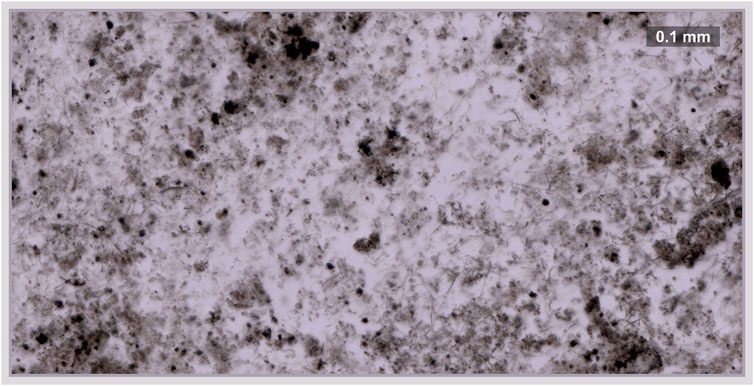
FIGURE 1. Transmitted light microscope image of the area (0.5 mm by 1 mm) chosen for the imaging. Dark patches represent the agglomeration of organic material. The scale bar indicates the size of features present in the sample (bar—100 μm). Two main components could be seen from the figure, filling milky host mineral (quartz) and organic material (dark lumps throughout the sample).

A spectral preprocessing routine was applied to every mass spectrum, which includes baseline correction, denoising, and averaging (Meyer et al., 2017; Lukmanov R. et al., 2021; Lukmanov R. A. et al., 2021). A single mass unit decomposition has been performed on the preprocessed mass spectra using Simpson integration of the mass peaks (Riedo et al., 2013a; Meyer et al., 2017). Overall, 260 single mass unit intensities (1–260 m/q) have been retrieved from the averaged mass spectra, and six additional mass pairs have been integrated to resolve some isobaric interferences, namely—²⁴Mg/C₂ (24 m/q), ⁵²Cr/C₄H₄ (52 m/q), and ¹³C/CH (13 m/q). After this step, mass spectra have been assigned with location indexes, forming a reduced volumetric grid of 266 mass intensities per 40,000 pixels and, for an averaged image, 266 mass intensities per 20,000 pixels. The SNR within the preprocessed mass spectra was identified to be ∼10³, which is limited by the noise floor and the dynamic range of the acquisition card. Furthermore, the dataset has been log-transformed and divided into subsets for imaging and low-dimensional analysis. The data reserved for the low-dimensional analysis (3D and 2D images) was z-score normalized and reduced with principal component analysis (PCA) down to the first 100 principal components.

Furthermore, to improve the image quality and readability, a volumetric dataset was interpolated from the original size (100 pixels by 200 pixels^∗2 layers) up to 250 pixels by 500 pixels^∗5 layers using inverse distance interpolation (Lu and Wong, 2008). Low-intensity zones of the imaged isotopes have been made translucent to improve the visibility of spatial heterogeneity. The inverse distance interpolation has been performed using the log-transformed data; thus, the color changes present in the pictures are logarithmic (base 10). Overall, using the data preprocessing routine, we have calculated volumetric maps of isotopes of interest. Each volumetric map is represented by 625000 voxels, which provides enough resolution to see the small discrepancies within the analyzed area. The volumetric maps characterize the uppermost layer (nm-scale) of the Gunflint sample (note that the Z-scale in element distribution maps was exaggerated). It has to be mentioned, however, that due to the sharp difference in the absorption properties of the investigated microfossils and host material (quartz), differences can be observed in the amount of the ablated material.

The dataset prepared for the low-dimensional analysis (normalized and PCA reduced to the first 100 components) was further analyzed using the uniform manifold approximation and projection (UMAP) method. The UMAP provides dimensionality reduction and groups similar spectra together in such a way that distances between observations in the low dimensions should approximate the original distance in the high dimensions. Here, we outline some of the sub-steps of the method; for a full and thorough description, we refer to the original UMAP manuscript (McInnes et al., 2018).

As in many other manifold learning methods, the UMAP algorithm tries to preserve small distances, thus recovering the local connectivity of data and its intrinsic dimensionality. In the first stage of the algorithm, similarity graph construction is performed using the approximate nearest neighbor (NN) descent (Dong et al., 2011), implemented within the UMAP (using the small minimal distance of 0.1, 5 nearest neighbors and cosine distance as a metric). Although the recall rate of nearest neighbors is reported to be high, it is not exact. The approximate NN search makes the algorithm fast, but it also includes the possibility of small mistakes in the determination of nearest neighbors. Even though exact solutions exist, for example, the graphics processing unit (GPU)–accelerated UMAP implementation provides such an option (Nolet et al., 2020), and approximate NN-search within the original UMAP-learn python implementation (McInnes et al., 2018) provides enough accuracy for the typical fs-LIMS tasks. Furthermore, in the second stage, the algorithm weighs the nearest neighbors and forms the weighted NN-graph using smoothing kernels that adapt to the local neighborhood. In the third and last stage, UMAP performs graph optimization by running a stochastic gradient descent for a determined number of epochs, decreasing the loss between low-dimensional and high-dimensional distances. The end stage (stochastic gradient descent) essentially represents the force-directed type optimization of the weighted neighborhood graph. The starting positions of the nodes are defined by Laplacian eigenmaps (spectral embedding) (Belkin and Niyogi, 2003). The usage of spectral embedding as an initialization step provides a good means for improved preservation of the global structure of the investigated manifold (Kobak and Linderman, 2019). The final step of the UMAP algorithm performs the embedding of the graph into a new coordinate system, which better reflects the similarity of n-dimensional vectors. Furthermore, to define the classes from the low-dimensional embeddings, a density-based hierarchical data clustering method (HDBSCAN) (Campello et al., 2013; McInnes et al., 2017) was used which provides a clustering hierarchy and derives clusters of spectra that share a significant degree of similarity. And last, for the derivation of reduced topological representations (in the form of a network) of the UMAP embedding, a Mapper algorithm (Singh et al., 2007; Van Veen et al., 2019) was used, which covers the original data with overlapping filter functions that are used to form the network and capture local connectivity of the data.

Results

The mass spectrometric investigation of the Gunflint chert sample using the high mass resolution fs-LIMS instrument yielded a large amount of data—266 volumetric mass intensity maps. Since most of the known Gunflint organic material is in a high preservation state (Alleon et al., 2016; Alleon et al., 2017), we have used ¹²C as an indicator of the organic material. Figure 2A shows the distribution of the ¹²C signal acquired from the Gunflint chert sample. The map reveals a high degree of co-occurrence between ¹²C intensities and the distribution of dark organic material identified using optical microscopy (Figure 1). The middle panel in Figure 2 shows the distribution of ³¹P intensities, which also reveals a relatively high degree of co-occurrence with ¹²C and with the distribution of organic matter (from the optical picture of the Gunflint chert, Figure 1 and lower panel in Figure 2). However, ³¹P is mostly present only within the areas of high ¹²C concentrations, which indicates that for the most part, ³¹P remained below the limit of detection.

FIGURE 2

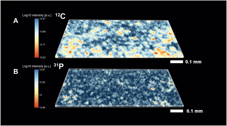
FIGURE 2. Volumetric isotope distribution maps from the Gunflint chert. (A)—distribution of ¹²C (red color indicates higher concentrations; see the scale bar on the left). (B)—distribution of ³¹P (red color indicates higher concentration). To compare maps with the optical image, see Figure 1. It is to be noted that the distribution of organic material and maps of ¹²C and ³¹P correlate relatively well with each other.

The co-occurrence of these two elements (¹²C and ³¹P) indicates that the measured elements are originating from the same source material (Cloud, 1965; Awramik and Barghoorn, 1977; Wacey et al., 2013; Lepot et al., 2017; Wiesendanger et al., 2018). However, there is a large part of the sample where we have observed a noisy distribution of both elements, and therefore, it is hard to definitively conclude where exactly the areas with organic carbon are located. Moreover, the host mineral (quartz) and the organic matter seem to be fused from the visual analysis of the intensity maps (note the cloudy areas where intensities fuse out). Similarly, the histogram of carbon intensities (see Supplementary Information) could be characterized as a skewed distribution, where the spectral ¹²C intensities transition from the noise level to the intensities with ¹²C saturation. A similar distribution could be observed for the ³¹P and other elements, where we do not observe any clear distinction between two separate entities—host (quartz) and organic material. Thus, identification of organic spectra solely on the basis of the presence of specific elements is possible for the high-intensity end members of the distributions, but localization of the exact boundary between the two classes is very challenging.

Figure 3 shows three panels with different isotope distribution maps. The upper panel shows the distribution of ³²S isotope intensities. One can note the presence of multiple bright spots on the map that indicate the presence of features chemically distinct from the host entities. In the upper part of the chemical map, we have identified an³²S-saturated area, which likely represents a pyritic (FeS₂) inclusion (see further in the text and SI), intermixed with organic material (a relatively bright spot in the ¹²C map as well, Figure 2). However, this position could also represent a small pod of pyritized microfossils, such as previously reported in (Wacey et al., 2013), but it could also be other S-containing minerals trapped within the organic material. In addition to the feature described above, we have observed another bright area saturated in ³²S, which is located in the lower-left part of the sample. One can compare the location of this spot with the map of ¹⁰⁷Ag, shown in the middle panel (Figure 3). The exact spatial localization of ³²S and ¹⁰⁷Ag indicates that it could be a sulfide inclusion, such as acanthite (Ag₂S), which again, seems to be sampled with organic remains. However, spatial co-localization of Ag and S within this bright area can also be some other more complex mineral or metallic aggregates sampled with other entities. The third bright area that could be observed from the ³²S map is located on the lower right side of the map. In addition to the bright spots in the sample, one can observe a fine-grained noise distribution throughout the sample.

FIGURE 3

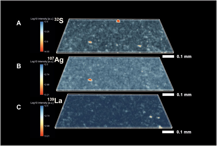
FIGURE 3. Volumetric isotope distribution maps of ³²S, ¹⁰⁷Ag, and ¹³⁹La from the Gunflint chert. (A) Distribution of the ³²S indicates the presence of localized S-enriched spots. Smaller intensities of ³²S co-occur with ¹²C (Figure 2). (B) Distribution of ¹⁰⁷Ag. (C) Distribution of ¹³⁹La in the Gunflint chert. The red color indicates higher intensities; the translucent blue indicates lower intensities of the investigated peaks.

The middle panel of Figure 3 shows the distribution of ¹⁰⁷Ag intensities. In contrast to the inclusions of S, silver mineralization appears to be relatively rare and localized only in one spot. The jittery fine signal in the background represents the noise. The third map shown in Figure 3 presents the distribution of ¹³⁹La intensities. The brightest spots in the lower right part of the volumetric map indicate the localization of spots enriched in ¹³⁹La.

The analysis of the full volumetric dataset to search for potentially missing “inclusions” (chemically distinct entities in the bulk of the sample) will result in a high workload (260 maps for comparison) and likely be counterproductive since one would need to correlate many specific elements to the given bright spots spatially. In addition, it is clear from the optical investigation of the thin section that there are two main compounds in the sample (organic material and the milky host). However, from the presented chemical maps of ¹²C and ³¹P, it is not clear where to define the borderline within the intensity profiles, which will outline the cutoff value for different compounds. In addition, any hand-picked cutoff value will be artificial as no clear intensity borderline between compounds can be seen on the chemical maps (Figure 2).

To solve this issue, the spectral dataset can be compared in terms of distances and analyzed using the k-NN (k-neighborhood graph) framework, assuming that similar minerals and compounds will yield small pairwise distances and, therefore, high similarity of ionization profiles. Thus, in order to find similar spectra and infer compound diversity, we performed an analysis of the fs-LIMS imaging data using the cosine distance and UMAP manifold learning method.

Figure 4A shows 40′000 (2 layers) fs-LIMS mass spectra (every data point is a composite mass spectrum) sampled from the original 260-dimensional space and reduced down to three dimensions using UMAP. The structure of the embedding outlines the chemical heterogeneity of the investigated area. The colors assigned to the data points show the distribution of the ¹²C intensities on the low-dimensional manifold. The structure of the node coordinates in the similarity network indicates the presence of three large groups: 1) the group of spectra at the bottom of the embedding that was interpreted to be from matrix mineralogy (quartz mineral). 2) The extended body of spectra in the upper part of the embedding was interpreted as spectra from organic material (OM). 3) A smaller group of spectra with a more complicated structure. These spectra were registered from various entities with more complex chemistry, such as spectra with enhanced S, Ag, and La (denoted as spectra with enhanced metallicity—see further in the text). The distribution of the ¹²C intensities in the OM cluster indicates that OM has variance in its structure—some are highly enriched in ¹²C and some are relatively depleted. The cluster of inclusions outlined in the figure reveals a high degree of ¹²C saturation (compared to quartz) and a relatively high proximity to the OM cluster, which indicates that spectra registered from these locations are a mixture between OM and some additional chemistry (see further in the text).

FIGURE 4

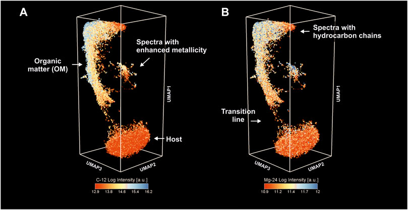
FIGURE 4. Low-dimensional proximity of the fs-LIMS spectra. The individual data points represent a single mass spectrum. Full volumetric (40,000 mass spectra, 2 layers) data have been considered for the analysis. Note the presence of three large clusters. (A) Proximity of fs-LIMS spectra colored according to the ¹²C intensities. Clusters associated with the microfossils and inclusions reveal a high level of ¹²C saturation. (B) Proximity of fs-LIMS spectra colored according to the ²⁴Mg intensities.

The panel on the right, Figure 4B, reveals the same embedding as in the left panel but colored using the ²⁴Mg intensities. In contrast to the ¹²C intensities, ²⁴Mg represents a trace element that is consistently present in the OM cluster. The spectra identified from the cluster with enhanced metallicity also show a relatively high degree of ²⁴Mg ion yield, indicating that it could be a major component in some of these compounds. The so-called “transition line,” Figure 4B, indicates a detached progression of spectral similarity between the host and OM. It is interesting to note that the structure of the OM group changes from relatively low ¹²C intensities up to the point of ¹²C saturation and subsequent hydrocarbon chain formation, as denoted in Figure 4B.

Figure 5 shows the distribution of ³²S (Figure 5A) and ³¹P (Figure 5B) intensities within the same UMAP embedding. The elevated concentrations of S and P coincide with the locations of a high C signal (although much weaker than ¹²C). Relatively low intensities of these elements indicate that P and S are present as trace elements. For example, the cluster of spectra with enhanced metallicity identified in Figure 4A reveals high S concentrations and likely represents the positioning of sulfides in the embedding. Thus, the elongated cluster of OM reveals multi-element enrichment of C, P, S, and Mg and also shows a high degree of spectral similarity (calculated on the basis of the full mass range) using the cosine metric.

FIGURE 5

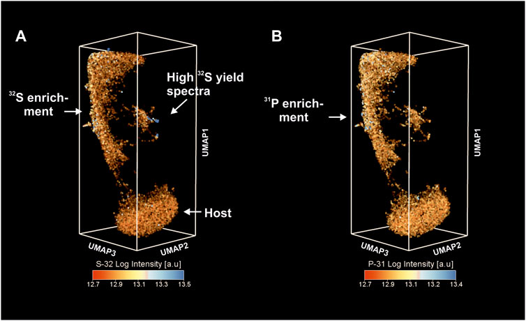
FIGURE 5. Low-dimensional proximity of fs-LIMS spectra revealed by UMAP. (A) Proximity of fs-LIMS spectra colored according to the ³²S intensities. Cluster associated with the OM reveals higher concentrations of ³²S. (B) Proximity of fs-LIMS spectra colored according to the ³¹P intensities. The cluster associated with the organic material reveals a relatively high level of ³¹P saturation.

Despite a few number of spectra in between main groups (see transition line in Figure 4B), it is possible to say that main clusters are easily separable. However, the smaller cluster of the spectra with enhanced metallicity shows a higher degree of complexity in the similarity structure—this complexity hints toward the presence of multiple compounds of varying chemistry (Figure 3). In order to segregate a single complex embedding into meaningful clusters with a high degree of similarity, we used a density-based, hierarchical clustering method (HDBSCAN) (Campello et al., 2013; McInnes et al., 2017). The method provides a clustering hierarchy, from which a simplified tree of significant clusters can be derived. Figure 6A shows the result of the clustering of all 40′000 mass spectra registered from the Gunflint sample (2 layers). One can note that we have identified four clusters in the first iteration of the algorithm. These clusters correspond to the large body of spectra registered from the OM (dark blue data points), from the matrix (quartz—purple points), from the spectra with enhanced metallicity (light blue points) (further, metallic cluster), and the REE spots (brown data points). The apparent similarities in the spectra that are transitioning from the OM to the metallic cluster indicate volumetrically mixed sampling with our laser (OM and portions of the metallic material). In order to improve the quality of the embedding for the cluster with enhanced metallicity, the mass spectra were separated from the main group and an additional UMAP embedding with a higher number of epochs (optimization iterations) using cosine distance and a small number of nearest neighbors (5-NN) was performed. The result of the embedding with interpretation is shown in Figure 6B. Since some of the clusters appeared to be fused into each other, but with distinguishable density profiles, kernel density estimates (KDE) for all identified clusters were calculated. Adding the previously described REE spots with quartz and OM, we have identified nine groups of spectra that are present in the investigated part of the Gunflint sample (0.5 mm by 1 mm), which reveal distinct similarity measures.

FIGURE 6

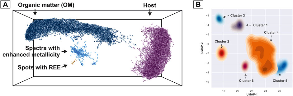
FIGURE 6. Clustering results of the UMAP scores. (A) Clustering of the dominant components. Data points are colored according to the assigned cluster. The individual data points represent a single mass spectrum. (B) Additional sub-clustering spectra are present in the group “Spectra with enhanced metallicity” as marked in Figure 6A. The clustering results reveal six groups of chemically distinct compounds.

The shape of the spectral embedding provides means for unsupervised classification of compounds; however, the understanding of the chemical discrepancies has to be ascertained with the original spectra. For the accurate characterization of identified classes, the spectra of every given class were averaged into single-composite mass spectra. Figure 7 reveals the averaged composite mass spectra from all identified clusters. All spectra shown in the figure are normalized to the maximal peak intensity—from 0 to 100 (a.u.). With the aim of delivering more details, spectral intensity profiles have been truncated down to the range of 0 to 50 (a.u.). In most cases, the most intense line was ²³Na, followed by ³⁹K (due to the low ionization energies of these elements) and ²⁸Si as the main constituents of the quartz matrix.

FIGURE 7

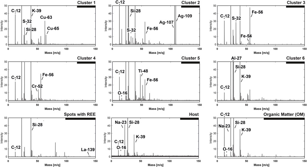
FIGURE 7. Spectral classes are identified from the UMAP embeddings. The spectra are averaged and normalized to the maximum peak intensity [0–100 (a.u.)]. To enhance the visibility of the small peaks, the intensity profiles are truncated to 50 (a.u.).

The first three clusters from the upper panel (Figure 7) reveal the chemical compositions where S co-occurs with some metallic species. The first cluster contains a significant amount of Cu and a noticeable peak of S (the upper left panel). The ³²S concentration is rather low; however, we have to consider the fact that the mass spectrum presented in the figure is an average of ∼100 pixels (200 laser shots), which provides a means for the drift of original ratios. In addition to the peaks of S and Cu, one can observe the presence of a relatively intense ¹²C peak and a significantly lower amount of Si and high K and Na. The presence of intense C and O and the proximity of spectra to the OM cluster within the main embedding (Figures 4–6) provide a piece of evidence that the spectra are registered from the mixture of OM, quartz matrix, and some Cu- and S-containing compounds. The next spectrum shown in the middle part of the upper panel is a composite spectrum from cluster number two. One may see that the spectrum contains significant peaks of Ag, followed by smaller peaks of Fe and S; High peaks of Si and C are likely registered from the quartz and OM [lines are well above 20 (a.u.)]. On the right side of the upper panel is shown the composite spectrum registered from cluster #3. Relatively high peaks of S and Fe with virtually no other significant metallic elements indicate that the spectra could be registered from for example, pyrite. However, other S- and Fe-containing minerals are possible. Again, the spectrum contains significant peaks of C and Si, potentially registered from the OM and quartz.

The second row of spectra in Figure 8 shows the classes that could be characterized as spectra from the organic material with significant metallic content (see further in the discussion), but without significant S content. The first element in the second row is the spectrum registered from cluster #4—the largest group of all among the identified compounds. It is interesting to note that the spectrum shows relatively high concentrations of Fe and Cr. Moreover, the spectrum presents the same elements present in the OM (carbon) and quartz (Si). Another group identified from the embedding, shown in the middle part of the second row, is cluster #5. The averaged composite spectrum reveals a high concentration of Ti as the main metallic constituent, followed by Fe. The last spectrum shown on the right side of the middle panel reveals the composition of cluster #6—which can be characterized by a high concentration of Al, followed by significantly reduced Fe and typical elements present in all groups—C, Si, Na, and K.

FIGURE 8

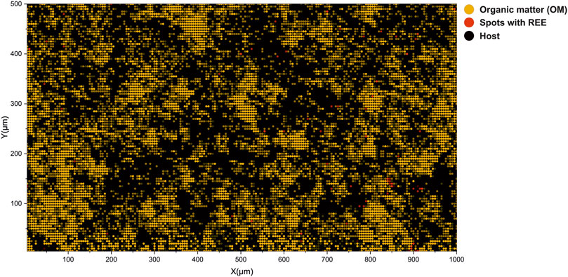
FIGURE 8. Interpretation of volumetric imaging results using cluster assignments calculated from low-dimensional embeddings. Yellow circles denote spectra registered by the OM. Gray circles denote spectra registered from the host mineral. Red circles denote locations of spectra registered from spectra with REE. It is to be noted that nodes are translucent and changes in the cluster assignment reflect the volumetric inhomogeneity of the sample.

The last row in Figure 7, the left panel, outlines the composition of spots with the REE—spectra with a relatively high concentration of ¹³⁹La, which was previously measured in connection with OM using the LIMS space–prototype instrument (Lukmanov R. A. et al., 2021). Among the main constituents of these inclusions, peaks of C, Al, and Si can be noted. The penultimate spectrum present in our interpretation model represents the composite spectrum from quartz mineral (spectrum from the large group host, Figures 4–6), or in other words, the silicate matrix of the Gunflint chert. The main element observed within the quartz mineral is Si, which is followed by K and Na, C, Ca, and minor levels of Si oxides. The spectrum represents an average of 100 pixels randomly sampled from the host (quartz) cluster. This was carried out to compare the spectrum with the equal number of spectra from the OM. This brings us to the last big cluster of OM—the spectrum presented in the last row and the right panel. As one may notice, the spectrum on the linear scale reveals a very similar chemical composition to the spectra presented before, with one notable difference—C is among the most abundant elements within this group (together with Na, Si, and K). In contrast, the latter (Si, K, and Na) are signatures of the host mineralogy that is co-ablated with the organic matter. As one can note, the clusters of spectra identified using the spectral embeddings and followed by density-based clustering identified meaningful subgroups of data with differing ionization profiles and chemical compositions. Overall, Figure 7 offers a visual assessment of the spectral dissimilarity and provides insight and intuition into the mechanics of spectral proximity. The interpretation of the UMAP embeddings, in short, follows the outlined logic. As soon as the laser hits the spot with the diluted organic remains, the output spectrum, even with low volumetric sampling, will form complex multipeak spectra, which in turn will yield a low similarity rank in comparison with the host spectra.

Spatial Interpretation of the Volumetric Maps.

In previous sections, the description of low-dimensional embeddings of the imaging dataset (two layers) was provided and a description of the identified clusters. It was shown that by using the cosine spectral distance, it was possible to advance to the identification of various compounds and entities present in the complex mass spectrometric data. In contrast to the “classical” data analysis, where one has to compare distributions of the various ion yields and try to solve the classification problem using probabilistic approaches (i.e., using logistic regression), relational data analysis provides a means to find more details and structure within complex datasets. For example, the popular ordination method, PCA, does not provide any clear boundaries between different classes for the given dataset, contrary to the UMAP embedding results. However, the grouping of spectra into clusters still lacks the spatial aspect. In order to understand how various clusters are spatially localized, the cluster map shown in Figure 8 can be utilized. The figure illustrates the distribution of the first three clusters. Laser ablation positions that are identified to be from the OM are colored with yellow nodes. The spectra clustered as inclusions with REE are colored orange. The gray nodes are sampled from the quartz matrix. To compare the distribution of the OM on the interpretation map and the optical image, see Figure 1. As one may note, the spatial localization of the OM largely follows the same structure captured in the optical image. The data points with dimmed colors represent the spatial difference in the class assignment. The localization of the REE spots largely follows the initial interpretation made on the basis of the chemical maps (Figure 3).

Figure 9 reveals the spatial localization of the six remaining clusters. The interpretation map presented in this figure shows only the second layer due to the fact that data from the surface contain very few metallic spectra and, therefore, will only clutter the figure. The white nodes are visualized as spectra from the cluster #1 with high Cu and S. The blue nodes localized in the lower left part of the sample are registered from cluster #2 (Ag rich spots). The red nodes, mainly localized in the upper part of the picture, represent the spectra registered from cluster #3 (Fe- and S-rich). The yellow nodes dispersed throughout the picture represent the spatial localization of the Fe-rich spectra (cluster #4). The green nodes represent cluster #5 with high Ti, and the purple nodes represent the spectra from the last cluster (#6), with high Al content. It is to be noted that all previously described bright spots (Figure 3) are present in the final interpretation map. Another noteworthy fact is that the spectra located on the upper layer, in most cases, belong to the group of OM. In general, the spatial distribution of the clusters reflects the fact that Fe-rich clusters are the most dominant among other metals.

FIGURE 9

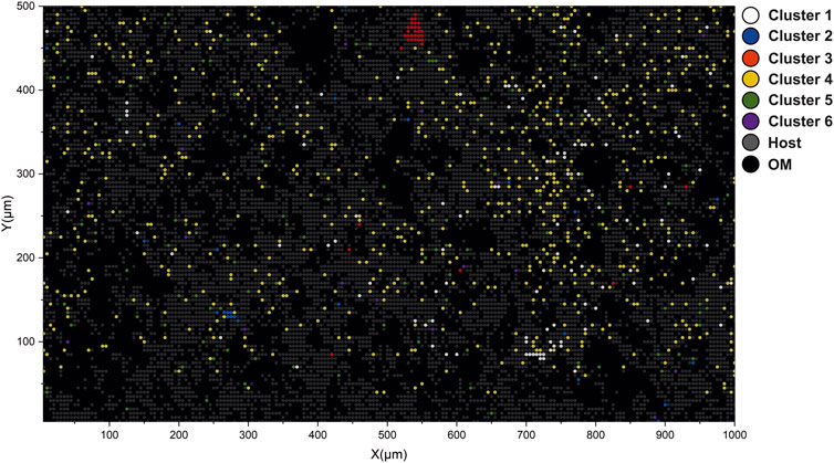
FIGURE 9. Interpretation map of the bottom layer. Circles denote laser ablation spots; color denotes class assignment.

Averaging Dynamics and Secondary Features Derived from the Topology of the Spectral Proximity Networks.

In addition to the three-dimensional UMAP embedding of the image, we have applied the Mapper algorithm (Singh et al., 2007) to capture the internal topology of the network using the Python Kepler Mapper implementation (Van Veen et al., 2019). Here, we will provide only a short description of the algorithm; for a full account of the inner workings of the algorithm, we refer the reader to the original publication (Singh et al., 2007) and an introductory article on topological data analysis (Carlsson, 2009). In general, the construction of the Mapper networks often trails the following logic: the first step typically includes a calculation of a low-dimensional representation of the original n-dimensional observations (by using neighborhood graphs or ordination methods). Furthermore, reduced observations are often combined with other metrics that capture outliers, density, and irregularities in the data (KDE, etc.). The objective variables (can be PCA or UMAP scores) are binned into a user-defined number of overlapping filter functions. The distribution of the data points within localized bins is further clustered using the clustering algorithm [specific choice is task-dependent (Pedregosa et al., 2011)]. The nodes that share the same observations are connected with an edge, and the output network is typically visualized using force-directed layouts. Furthermore, the output network is colored according to the target variable, which provides the interpretation and hot-spot analysis. The transformation of the original UMAP scores to the network provides several additional benefits that can be useful in further downstream machine learning tasks. Depending on the chosen resolution, the Mapper networks are able to better capture the global topology and provide some degree of tolerance to the noise and flexibility to combine various metrics. Another beneficial side of the Mapper networks is the fact that it is possible to visualize an arbitrary number of dimensions within a single complex network. Most useful applications are typically two to three dimensional; however, it is possible to visualize 4 to 5-dimensional datasets by using the four and five-hypercubes as filter functions. Such networks can provide an additional level of detail or coarseness as needed. The challenge of using the high-dimensional filter functions is that they grow with power and typically form large graphs, which are not always convenient to work with. However, the main advantage of the Mapper networks is that they can significantly reduce the number of data points while preserving the main structural details.

The fs-LIMS is a point-to-point chemical characterization method that provides the capability to perform depth profiles and volumetric estimates of any solid material. However, the ablation rate of investigated materials depending on the applied laser wavelength might vary, so the characterization of very small inclusions (micro-to nanograins) can be affected by the number of applied laser shots. For example, if a majority of the investigated material is ablated with the first laser shot, further averaging of additional laser shots is counterproductive because the target material is already removed from the sample. Using the assumption that some features (and the mineralization related to them) might be of nm size in depth, we decided to recalculate the new embeddings for the averaged dataset (one layer data) and compare how the structure of the proximity networks will change. Figure 10 shows the spectral proximity network computed on the UMAP scores (using an increased number of epochs, 5 NN, and a cosine distance) on the 2-layer dataset (40,000 mass spectra, 260 single unit masses). The first three UMAP dimensions have been used as filter functions divided into 40 windows with 30 percent overlap and further clustered using the density-based clustering algorithm (DBSCAN) within the overlapping voxels (Ester et al., 1996). The output undirected graph was further visualized in the open-source graph visualization platform Gephi (Bastian et al., 2009) using the ForceAtlas2 layout algorithm (Jacomy et al., 2014), and edges are colored according to the degree of the nodes (blue—higher degree, yellow and red—smaller degree, see the scale bar with the shape of the degree distribution). The network in Figure 10 reveals the structure of the cosine spectral proximities and indicates the complexity of that metric present in the dataset. The structure of the network shows disjoint clusters that consist of three main components: the host cluster shows a uniform radial structure, indicating that spectra from this cluster have less internal variability in intensity profiles. In contrast, the spectra from the cluster of OM indicate the gradual change of the spectral proximity and, thus, form a more complex shape, which reflects the change in the volumetric ablation and ionization. And last, the cluster from spectra with enhanced metallicity shows a complex internal topology, which indicates the complexity of the chemical compositions of these spectra.

FIGURE 10

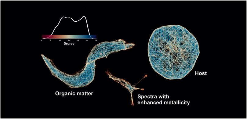
FIGURE 10. Spectral proximity network of the partially averaged mass spectrometric image (40′000 mass spectra 260 single unit masses). The networks are colored according to the node degree (the degree of a node is the number of edges connected to the node).

As mentioned in the Methods section, in addition to the original volumetric dataset, an averaged mass spectrometric image was calculated, which contains the five single-laser shots per pixel, averaged for every given pixel forming a dataset that consists of 20′000 mass spectra (single layer). Figure 11 shows the spectral proximity network calculated from a single-layer (fully averaged) mass spectrometric image but visualized using the Yifan Hu graph layout algorithm (Hu, 2005) and calculated using the same hyperparameters. The change of the layout algorithm was motivated by the artifactual visualization of microfossil clusters using the ForceAtlas2. The network (Figure 11) shows the distribution of node degrees on the same network (see the scale bar with the shape of the degree distribution). As shown in Figure 11, the global structure of the similarity graphs remained very similar—the two biggest components are easily separable. However, one can see that the transition line between the host and OM (Figures 10, 11) appeared in the proximity structure after averaging more spectra (five single-laser shot spectra), and the fine structure of metallic spectra was reduced to a single spike, which now shows the linkage to the transition line, and thus to the OM. An interpretation of this observation could be made in the following way: the pairwise spectral distances with an increased averaging are getting smaller due to the volumetric domination of the quartz matrix or OM (depending on the pixel location); thus, the spectra from different classes are becoming more fused into each other. It was also mentioned that the secondary metrics calculated from the spectral similarity networks might be of use in the downstream machine learning tasks. For example, Figure 10 shows three distinct clusters with an identifiable degree of centrality that can be further used as a selective and descriptive feature together with their UMAP scores. The topological structure of the graph itself also provides very important information, that is, the eigenvalue spectrum of the normalized just graph Laplacian describes the network’s structure on a global level (de Lange et al., 2014) just by using one metric, without referring to individual nodes or connections. For example, the characteristic “neck” of the transition structure from the host (quartz matrix) toward the microfossils has been observed in our previous work on the Gunflint microfossils using the space-type mass-spectrometer (Lukmanov R. et al., 2021). Overall, the current dataset generated with the LMS-GT instrument can be easily segregated into clusters of Precambrian OM vs. the host. Thus, our approach can be of high utility, for example, in dealing with highly chemically diverse samples.

FIGURE 11

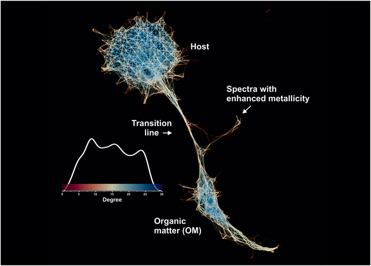
FIGURE 11. Spectral proximity network of the fully averaged mass spectrometric image (20′000 mass spectra 260 single unit masses). The network is colored according to the degree of nodes in the network. The blue colors indicate nodes with a higher degree. It is to be noted that the fine transition structure gets thicker with the higher average number of laser shots. The metallic clusters also lost their fine structure, which reflects the importance of good volumetric sampling.

Discussion

The OM, which constitutes a significant part of the sample, was detected by measuring the abundant signal of ¹²C, with smaller concentrations of ³¹P. An additional spectral embedding using the cosine distance measure revealed that the OM forms a distinct group of mass spectra. The structural composition of the OM indicates that it is relatively homogenous throughout the investigated area of the sample (Figures 10, 11). Using the matrix factorization (PCA) and further low-dimensional embeddings (UMAP), it was shown that metallic inclusions reveal a certain level of proximity to the OM. The most abundant group among inclusions identified as Fe-rich spectra – cluster #4 (Figures 7, 9) likely represents some Fe-oxides. The presence of Greenalite, nano-minerals has recently been identified within specific morphospecies (Lepot et al., 2017) in the Gunflint OM. Furthermore, the ionization of small portions of the OM, together with Fe-oxides and the surrounding silicate matrix, can explain a certain proximity to the main OM cluster. The abundant Fe, Si, and O signals observed in the spectrum (Figure 7—middle left panel) are supportive of that conclusion. Interestingly, high Fe concentrations within this group were also accompanied by relatively high Cr peaks, which can indicate a relatively widespread presence of Cr-oxides as well. However, our observations show that the metallicity in the investigated Gunflint area is broader and reveals Cu, Ti, Al, and Ag mineralization. Some of these compounds are likely to be sulfides such as pyrite, covellite, and acanthine, although exact mineralogical identifications will require additional multimethod correlative studies. The presence of REE was mainly manifested with La, whereas other REE elements remained below the detection limit. The REEs can be present in sedimentary phosphates entrapped in the bulk of the sample. However, again, the identification of the exact mineralogical form of these compounds needs further study.

Here, we also have to report the caveats related to this work. The spectral profile of the quartz mineral shown in Figure 7 indicates that the total ion yield is a lot smaller in comparison to the spectra registered by other groups (note the brushier baseline in the spectrum). This observation could be explained by the usage of the fs-IR 775-nm laser. The clean quartz material is nearly transparent for the given wavelength, and therefore more energy is required to be deposited on the surface of the sample (Lukmanov et al., 2022). In contrast to quartz, organic material is more absorptive of the given wavelength and can yield a higher SNR even with smaller applied energies. Unequal laser fluences required for the balanced ionization of both materials can be solved by using nonlinear beta barium borate crystals that can multiply the output frequencies of the laser, going deeper into the UV range. Another potential pitfall concerns the surface quality of the sample. The orthogonal to the sample laser focusing implemented in our current setup provides a fixed position of the laser focus; thus, changes in the topography of the sample can induce changes in the subsequent ionization. Such changes can affect the output image quality by forming an ion yield that is not related to the chemistry of the investigated sample. Another phenomenon that can affect the image quality and the quality of embeddings is the ablation depth and quantification of the layers. In cases where deep craters are required, fs-LIMS can yield declining ion intensities due to the change in the depth of ablation as material will not be placed in the focal plane of the laser. Thus, spectral similarity networks can segregate layers instead of compounds. Preliminary calibration studies are necessary to avoid such artifacts. Further studies could also be improved by the usage of beam blanking technology, which was shown to improve the detection limits of various elements (Gruchola et al., 2022).

The spectral decomposition used in this work covers only single unit masses, except for Mg and Cr lines. Thus, additional scripts are required for future campaigns to extract finer spectral information, resolving the majority of the isobaric interferences. In addition, algorithmic baseline subtraction and denoising on large spectral libraries can sometimes yield artifacts that can be manifested in further downstream analysis. The calculation of spectral embeddings, as was mentioned before, was carried out by using the cosine metric. However, a great variety of other metrics are available, and their impact on the aspects of spectral similarity needs to be assessed. Moreover, the number of neighbors (N) in the construction of the neighborhood graph has a profound effect on the structure of the embedding. By choosing a large N, one can approximate more of the global structure or, alternatively, emphasize more of the local neighborhood by reducing N. In general, choosing the right N requires some trial and error; however, the reader has to keep in mind that provided embeddings are parameter-dependent. In addition, the proximity of nodes in the output embedding can have no physical meaning if there is no edge between them (e.g., if distances are not defined, see SI for connectivity graphs). Thus, the analytical assessment of the graph connectivity is helpful in the interpretation step of the UMAP embeddings or any other graph-based manifold learning method. A similar situation affects the construction of the Mapper networks, where a variety of hyperparameters are present, for example, the number of filter function windows, percentage of overlap, and hyperparameters of the clustering algorithms.

Conclusion

Large and unstructured chemical information (mass spectra) often poses critical constraints on the quality of information that can be retrieved from a given experiment. In this contribution, we demonstrated that it is possible to convolve complex mass spectrometric signals into compact networks using sequential data and dimensionality reduction techniques. Such networks can reveal new and informative properties of mass spectrometric measurements, outlining the diversity of compounds and their homogeneity. The low-dimensional UMAP embeddings calculated from the fs-LIMS imaging data yielded nine distinct clusters and a strong separation between the organic matter and inorganic host spectra recorded from the 1.88 Ga Gunflint chert. The average dynamics of the imaging data provide an additional perspective on the preservation of the structural information. In conclusion, fs-laser ionization mass spectrometry combined with manifold learning techniques provides a powerful analytical framework and is capable of accelerating knowledge extraction from complex, chemically diverse samples.

Data Availability Statement

The original contributions presented in the study are included in the article/Supplementary Material; further inquiries can be directed to the corresponding author.

Author Contributions

RL performed the experiments and data analysis. RL wrote the main manuscript. All authors reviewed and revised the manuscript.

Funding

Open access funding was provided by the University of Bern.

Conflict of Interest

The authors declare that the research was conducted in the absence of any commercial or financial relationships that could be construed as a potential conflict of interest.

Publisher’s Note

All claims expressed in this article are solely those of the authors and do not necessarily represent those of their affiliated organizations, or those of the publisher, the editors, and the reviewers. Any product that may be evaluated in this article, or claim that may be made by its manufacturer, is not guaranteed or endorsed by the publisher.

Acknowledgments

The authors would like to acknowledge the financial support from the Swiss National Science Foundation. DW acknowledges funding from the Australian Research Council via a Future Fellowship Grant.

Supplementary Material

The Supplementary Material for this article can be found online at: https://www.frontiersin.org/articles/10.3389/frspt.2022.718943/full#supplementary-material

References

Alleon, J., Bernard, S., Le Guillou, C., Daval, D., Skouri-Panet, F., Pont, S., et al. (2016). Early Entombment within Silica Minimizes the Molecular Degradation of Microorganisms during Advanced Diagenesis. Chem. Geology. 437, 98–108. doi:10.1016/j.chemgeo.2016.05.034

CrossRef Full Text | Google Scholar

Alleon, J., Bernard, S., Le Guillou, C., Marin-Carbonne, J., Pont, S., Beyssac, O., et al. (2017). Molecular Preservation of 1.88 Ga Gunflint Organic Microfossils as a Function of Temperature and Mineralogy. Nat. Commun. 8 (1), 16147. doi:10.1038/ncomms16147

PubMed Abstract | CrossRef Full Text | Google Scholar

Awramik, S. M., and Barghoorn, E. S. (1977). The Gunflint Microbiota. Precambrian Res. 5, 121–142. doi:10.1016/0301-9268(77)90025-0

CrossRef Full Text | Google Scholar

Azov, V. A., Mueller, L., and Makarov, A. A. (2020). Laser Ionization Mass Spectrometry at 55: Quo Vadis? Mass Spectrom. Rev. 41 (1), 100–151. doi:10.1002/mas.21669

PubMed Abstract | CrossRef Full Text | Google Scholar

Barghoorn, E. S., and Tyler, S. A. (1965). Microorganisms from the Gunflint Chert. Science 147, 563–575. doi:10.1126/science.147.3658.563

PubMed Abstract | CrossRef Full Text | Google Scholar

Bastian, M., Heymann, S., and Jacomy, M. (2009). “Gephi: an Open Source Software for Exploring and Manipulating Networks,” in Proceedings of the International AAAI Conference on Web and Social Media.

CrossRef Full Text | Google Scholar

Becht, E., Mcinnes, L., Healy, J., Dutertre, C.-A., Kwok, I. W. H., Ng, L. G., et al. (2019). Dimensionality Reduction for Visualizing Single-Cell Data Using UMAP. Nat. Biotechnol. 37, 38–44. doi:10.1038/nbt.4314

CrossRef Full Text | Google Scholar

Belkin, M., and Niyogi, P. (2003). Laplacian Eigenmaps for Dimensionality Reduction and Data Representation. Neural Comput. 15, 1373–1396. doi:10.1162/089976603321780317

CrossRef Full Text | Google Scholar

Brasier, M. D., Green, O. R., Jephcoat, A. P., Kleppe, A. K., Van Kranendonk, M. J., Lindsay, J. F., et al. (2002). Questioning the Evidence for Earth's Oldest Fossils. Nature 416, 76–81. doi:10.1038/416076a

PubMed Abstract | CrossRef Full Text | Google Scholar

Brasier, M. D., and Wacey, D. (2012). Fossils and Astrobiology: New Protocols for Cell Evolution in Deep Time. Int. J. Astrobiology 11, 217–228. doi:10.1017/s1473550412000298

CrossRef Full Text | Google Scholar

Campello, R. J., Moulavi, D., and Sander, J. (2013). “Density-based Clustering Based on Hierarchical Density Estimates,” in Pacific-Asia conference on knowledge discovery and data mining (Springer), 160–172.

CrossRef Full Text | Google Scholar

Carlsson, G. (2009). Topology and Data. Bull. Amer. Math. Soc. 46, 255–308. doi:10.1090/s0273-0979-09-01249-x

CrossRef Full Text | Google Scholar

Cloud, P. E. (1965). Significance of the Gunflint (Precambrian) Microflora: Photosynthetic Oxygen May Have Had Important Local Effects before Becoming a Major Atmospheric Gas. Science 148, 27–35. doi:10.1126/science.148.3666.27

PubMed Abstract | CrossRef Full Text | Google Scholar

Cosmidis, J., and Templeton, A. S. (2016). Self-assembly of Biomorphic Carbon/sulfur Microstructures in Sulfidic Environments. Nat. Commun. 7, 12812. doi:10.1038/ncomms12812

PubMed Abstract | CrossRef Full Text | Google Scholar

Cui, Y., Moore, J. F., Milasinovic, S., Liu, Y., Gordon, R. J., and Hanley, L. (2012). Depth Profiling and Imaging Capabilities of an Ultrashort Pulse Laser Ablation Time of Flight Mass Spectrometer. Rev. Sci. Instrum 83, 093702. doi:10.1063/1.4750974

PubMed Abstract | CrossRef Full Text | Google Scholar

Cui, Y., Bhardwaj, C., Milasinovic, S., Carlson, R. P., Gordon, R. J., and Hanley, L. (2013). Molecular Imaging and Depth Profiling of Biomaterials Interfaces by Femtosecond Laser Desorption Postionization Mass Spectrometry. ACS Appl. Mater. Inter. 5, 9269–9275. doi:10.1021/am4020633

CrossRef Full Text | Google Scholar

De Koning, C. P., Gruchola, S., Riedo, A., Wiesendanger, R., Grimaudo, V., Lukmanov, R., et al. (2021a). Quantitative Elemental Analysis with the LMS-GT; a Next-Generation LIMS-TOF Instrument. Int. J. mass Spectrom. 470, 116662. doi:10.1016/j.ijms.2021.116662

CrossRef Full Text | Google Scholar

De Lange, S. C., De Reus, M. A., and Van Den Heuvel, M. P. (2014). The Laplacian Spectrum of Neural Networks. Front. Comput. Neurosci. 7, 189. doi:10.3389/fncom.2013.00189

PubMed Abstract | CrossRef Full Text | Google Scholar

Dong, W., Moses, C., and Li, K. (2011). “Efficient K-Nearest Neighbor Graph Construction for Generic Similarity Measures,” in Proceedings of the 20th international conference on World wide web, 577–586.

CrossRef Full Text | Google Scholar

Ester, M., Kriegel, H.-P., Sander, J., and Xu, X. (1996). “A Density-Based Algorithm for Discovering Clusters in Large Spatial Databases with Noise”, in: Kdd). Vol. 96 (34), 226–231.

Google Scholar

García-Ruiz, J. M., Hyde, S. T., Carnerup, A. M., Christy, A. G., Van Kranendonk, M. J., and Welham, N. J. (2003). Self-assembled Silica-Carbonate Structures and Detection of Ancient Microfossils. science 302, 1194–1197. doi:10.1126/science.1090163

PubMed Abstract | CrossRef Full Text | Google Scholar

Grimaudo, V., Tulej, M., Riedo, A., Lukmanov, R., Ligterink, N. F. W., De Koning, C., et al. (2020). UV post-ionization Laser Ablation Ionization Mass Spectrometry for Improved Nm-Depth Profiling Resolution on Cr/Ni Reference Standard. Rapid Commun. Mass. Spectrom. 34, e8803. doi:10.1002/rcm.8803

PubMed Abstract | CrossRef Full Text | Google Scholar

Grimaudo, V., Moreno-García, P., Riedo, A., López, A. C., Tulej, M., Wiesendanger, R., et al. (2019). Review-Laser Ablation Ionization Mass Spectrometry (LIMS) for Analysis of Electrodeposited Cu Interconnects. J. Electrochem. Soc. 166, D3190–D3199. doi:10.1149/2.0221901jes

CrossRef Full Text | Google Scholar

Gruchola, S., De Koning, C. P., Wiesendanger, R., Keresztes Schmidt, P., Riedo, A., Grimaudo, V., et al. (2022). Improved Limit of Detection of a High-Resolution Fs-LIMS Instrument through Mass-Selective Beam Blanking. Int. J. Mass Spectrom. 474, 116803. doi:10.1016/j.ijms.2022.116803

CrossRef Full Text | Google Scholar

House, C. H., Schopf, J. W., McKeegan, K. D., Coath, C. D., Harrison, T. M., and Stetter, K. O. (2000). Carbon Isotopic Composition of Individual Precambrian Microfossils. Geology 28, 707–710.

PubMed Abstract | CrossRef Full Text | Google Scholar

Hu, Y. (2005). Efficient, High-Quality Force-Directed Graph Drawing. Mathematica J. 10, 37–71.

Google Scholar

Huang, R., Yu, Q., Li, L., Lin, Y., Hang, W., He, J., et al. (2011). High Irradiance Laser Ionization Orthogonal Time-of-flight Mass Spectrometry: A Versatile Tool for Solid Analysis. Mass. Spectrom. Rev. 30, 1256–1268. doi:10.1002/mas.20331

PubMed Abstract | CrossRef Full Text | Google Scholar

Jacomy, M., Venturini, T., Heymann, S., and Bastian, M. (2014). ForceAtlas2, a Continuous Graph Layout Algorithm for Handy Network Visualization Designed for the Gephi Software. PloS one 9, e98679. doi:10.1371/journal.pone.0098679

PubMed Abstract | CrossRef Full Text | Google Scholar

Jolliffe, I. T., and Cadima, J. (2016). Principal Component Analysis: a Review and Recent Developments. Phil. Trans. R. Soc. A. 374, 20150202. doi:10.1098/rsta.2015.0202

PubMed Abstract | CrossRef Full Text | Google Scholar

Kobak, D., and Linderman, G. C. (2019). UMAP Does Not Preserve Global Structure Any Better Than T-SNE when Using the Same Initialization. bioRxiv, 2019.2012.2019.877522.

Google Scholar

Lepot, K., Addad, A., Knoll, A. H., Wang, J., Troadec, D., Béché, A., et al. (2017). , 8, 14890. doi:10.1038/ncomms14890Iron Minerals within Specific Microfossil Morphospecies of the 1.88 Ga Gunflint FormationNat. Commun.

PubMed Abstract | CrossRef Full Text | Google Scholar

Liang, Z., Zhang, S., Li, X., Wang, T., Huang, Y., Hang, W., et al. (2017). Tip-enhanced Ablation and Ionization Mass Spectrometry for Nanoscale Chemical Analysis. Sci. Adv. 3, eaaq1059–1059. doi:10.1126/sciadv.aaq1059

PubMed Abstract | CrossRef Full Text | Google Scholar

Ligterink, N. F. W., Grimaudo, V., Moreno-García, P., Lukmanov, R., Tulej, M., Leya, I., et al. (2020). ORIGIN: a Novel and Compact Laser Desorption - Mass Spectrometry System for Sensitive In Situ Detection of Amino Acids on Extraterrestrial Surfaces. Sci. Rep. 10, 9641. doi:10.1038/s41598-020-66240-1

PubMed Abstract | CrossRef Full Text | Google Scholar

Lu, G. Y., and Wong, D. W. (2008). An Adaptive Inverse-Distance Weighting Spatial Interpolation Technique. Comput. Geosciences 34, 1044–1055. doi:10.1016/j.cageo.2007.07.010

CrossRef Full Text | Google Scholar

Lukmanov, R. A., Tulej, M., Ligterink, N. F. W., De Koning, C., Riedo, A., Grimaudo, V., et al. (2021b). Chemical Identification of Microfossils from the 1.88-Ga Gunflint Chert: Towards Empirical Biosignatures Using Laser Ablation Ionization Mass Spectrometer. J. Chemometrics 35, e3370. doi:10.1002/cem.3370

CrossRef Full Text | Google Scholar

Lukmanov, R. A., Tulej, M., Wiesendanger, R., Riedo, A., Grimaudo, V., Ligterink, N. F. W., et al. (2022). Multiwavelength Ablation/Ionization and Mass Spectrometric Analysis of 1.88 Ga Gunflint Chert. Astrobiology. doi:10.1089/ast.2019.2201

CrossRef Full Text | Google Scholar

Lukmanov, R., Riedo, A., Wacey, D., Ligterink, N. F., Riedo, V., Tulej, M., et al. (2021a). On Topological Analysis of Fs-LIMS Data. Implications for In Situ Planetary Mass Spectrometry. Front. Artif. intelligence 119, 668163. doi:10.3389/frai.2021.668163

CrossRef Full Text | Google Scholar

Mcinnes, L., Healy, J., and Astels, S. (2017). Hdbscan: Hierarchical Density Based Clustering. Joss 2, 205. doi:10.21105/joss.00205

CrossRef Full Text | Google Scholar

Mcinnes, L., Healy, J., and Melville, J. (2018). Umap: Uniform Manifold Approximation and Projection for Dimension Reduction. arXiv preprint arXiv:1802.03426.

Google Scholar

Meyer, S., Riedo, A., Neuland, M. B., Tulej, M., and Wurz, P. (2017). Fully Automatic and Precise Data Analysis Developed for Time-Of-Flight Mass Spectrometry. J. Mass. Spectrom. 52, 580–590. doi:10.1002/jms.3964

PubMed Abstract | CrossRef Full Text | Google Scholar

Moreno-García, P., Grimaudo, V., Riedo, A., Tulej, M., Wurz, P., and Broekmann, P. (2016). Towards Matrix-free Femtosecond-Laser Desorption Mass Spectrometry for In Situ Space Research. Rapid Commun. Mass. Spectrom. 30, 1031–1036. doi:10.1002/rcm.7533

PubMed Abstract | CrossRef Full Text | Google Scholar

Neuland, M. B., Grimaudo, V., Mezger, K., Moreno-García, P., Riedo, A., Tulej, M., et al. (2016). Quantitative Measurement of the Chemical Composition of Geological Standards with a Miniature Laser Ablation/ionization Mass Spectrometer Designed Forin Situapplication in Space Research. Meas. Sci. Technol. 27, 035904. doi:10.1088/0957-0233/27/3/035904

CrossRef Full Text | Google Scholar

Nolet, C. J., Lafargue, V., Raff, E., Nanditale, T., Oates, T., Zedlewski, J., et al. (2020).Bringing UMAP Closer to the Speed of Light with GPU Acceleration. arXiv preprint arXiv:2008.00325.

Google Scholar

Pearson, K. (1901). LIII. On Lines and Planes of Closest Fit to Systems of Points in Space. Lond. Edinb. Dublin Phil. Mag. J. Sci. 2, 559–572. doi:10.1080/14786440109462720

CrossRef Full Text | Google Scholar

Pedregosa, F., Varoquaux, G., Gramfort, A., Michel, V., Thirion, B., Grisel, O., et al. (2011). Scikit-learn: Machine Learning in Python. J. machine Learn. Res. 12, 2825–2830. doi:10.5555/1953048.2078195

CrossRef Full Text | Google Scholar

Planavsky, N., Rouxel, O., Bekker, A., Shapiro, R., Fralick, P., and Knudsen, A. (2009). Iron-oxidizing Microbial Ecosystems Thrived in Late Paleoproterozoic Redox-Stratified Oceans. Earth Planet. Sci. Lett. 286, 230–242. doi:10.1016/j.epsl.2009.06.033

CrossRef Full Text | Google Scholar

Riedo, A., Meyer, S., Heredia, B., Neuland, M. B., Bieler, A., Tulej, M., et al. (2013a). Highly Accurate Isotope Composition Measurements by a Miniature Laser Ablation Mass Spectrometer Designed for In Situ Investigations on Planetary Surfaces. Planet. Space Sci. 87, 1–13. doi:10.1016/j.pss.2013.09.007

CrossRef Full Text | Google Scholar

Riedo, A., Neuland, M., Meyer, S., Tulej, M., and Wurz, P. (2013b). Coupling of LMS with a Fs-Laser Ablation Ion Source: Elemental and Isotope Composition Measurements. J. Anal. Spectrom. 28, 1256–1269. doi:10.1039/c3ja50117e

CrossRef Full Text | Google Scholar

Riedo, A., Tulej, M., Rohner, U., and Wurz, P. (2017). High-speed Microstrip Multi-Anode Multichannel Plate Detector System. Rev. Scientific Instr. 88, 045114. doi:10.1063/1.4981813

CrossRef Full Text | Google Scholar

Rouillard, J., Van Kranendonk, M. J., Lalonde, S., Gong, J., and Van Zuilen, M. A. (2021). Correlating Trace Element Compositions, Petrology, and Raman Spectroscopy Data in the ∼3.46 Ga Apex Chert, Pilbara Craton, Australia. Precambrian Res. 366, 106415. doi:10.1016/j.precamres.2021.106415

CrossRef Full Text | Google Scholar

Sainburg, T., Mcinnes, L., and Gentner, T. Q. (2020). Parametric UMAP Embeddings for Representation and Semi-supervised Learning. arXiv preprint arXiv:2009.12981.

Google Scholar

Schopf, J. W., Kitajima, K., Spicuzza, M. J., Kudryavtsev, A. B., and Valley, J. W. (2018). SIMS Analyses of the Oldest Known Assemblage of Microfossils Document Their Taxon-Correlated Carbon Isotope Compositions. Proc. Natl. Acad. Sci. U.S.A. 115, 53–58. doi:10.1073/pnas.1718063115

PubMed Abstract | CrossRef Full Text | Google Scholar

Schopf, J. W., and Kudryavtsev, A. B. (2012). Biogenicity of Earth's Earliest Fossils: A Resolution of the Controversy. Gondwana Res. 22 (3-4), 761–771. doi:10.1016/j.gr.2012.07.003

CrossRef Full Text | Google Scholar

Singh, G., Mémoli, F., and Carlsson, G. E. (2007). Topological Methods for the Analysis of High Dimensional Data Sets and 3d Object Recognition. SPBG 91, 100. doi:10.2312/SPBG/SPBG07/091-100

CrossRef Full Text | Google Scholar

Stevens, A. H., Mcdonald, A., De Koning, C., Riedo, A., Preston, L. J., Ehrenfreund, P., et al. (2019). Detectability of Biosignatures in a Low-Biomass Simulation of Martian Sediments. Sci. Rep. 9, 9706. doi:10.1038/s41598-019-46239-z

PubMed Abstract | CrossRef Full Text | Google Scholar

Stewart, G. W. (1993). On the Early History of the Singular Value Decomposition. SIAM Rev. 35, 551–566. doi:10.1137/1035134

CrossRef Full Text | Google Scholar

Tulej, M., Ligterink, N. F. W., De Koning, C., Grimaudo, V., Lukmanov, R., Keresztes Schmidt, P., et al. (2021a). Current Progress in Femtosecond Laser Ablation/Ionisation Time-Of-Flight Mass Spectrometry. Appl. Sci. 11, 2562. doi:10.3390/app11062562

CrossRef Full Text | Google Scholar

Tulej, M., Lukmanov, R., Grimaudo, V., Riedo, A., De Koning, C., Ligterink, N. F. W., et al. (2021b). Determination of the Microscopic Mineralogy of Inclusion in an Amygdaloidal Pillow basalt by Fs-LIMS. J. Anal. Spectrom. 36, 80–91. doi:10.1039/d0ja00390e

CrossRef Full Text | Google Scholar

Tyler, S. A., and Barghoorn, E. S. (1954). Occurrence of Structurally Preserved Plants in Pre-cambrian Rocks of the Canadian Shield. Science 119, 606–608. doi:10.1126/science.119.3096.606

PubMed Abstract | CrossRef Full Text | Google Scholar

Van Der Maaten, L., and Hinton, G. (2008). Visualizing Data Using T-SNE. J. machine Learn. Res. 9.

Google Scholar

Van Veen, H., Saul, N., Eargle, D., and Mangham, S. (2019). Kepler Mapper: A Flexible Python Implementation of the Mapper Algorithm. Joss 4, 1315. doi:10.21105/joss.01315

CrossRef Full Text | Google Scholar

Van Zuilen, M. A., Lepland, A., and Arrhenius, G. (2002). Reassessing the Evidence for the Earliest Traces of Life. Nature 418, 627–630. doi:10.1038/nature00934

PubMed Abstract | CrossRef Full Text | Google Scholar

Wacey, D., Mcloughlin, N., Kilburn, M. R., Saunders, M., Cliff, J. B., Kong, C., et al. (2013). Nanoscale Analysis of Pyritized Microfossils Reveals Differential Heterotrophic Consumption in the ∼1.9-Ga Gunflint Chert. Proc. Natl. Acad. Sci. U S A. 110, 8020–8024. doi:10.1073/pnas.1221965110

PubMed Abstract | CrossRef Full Text | Google Scholar

Wacey, D., Eiloart, K., and Saunders, M. (2019). Comparative Multi-Scale Analysis of Filamentous Microfossils from the C. 850 Ma Bitter Springs Group and Filaments from the C. 3460 Ma Apex Chert. J. Geol. Soc. 176, 1247–1260. doi:10.1144/jgs2019-053

CrossRef Full Text | Google Scholar

Wacey, D., Menon, S., Green, L., Gerstmann, D., Kong, C., Mcloughlin, N., et al. (2012). Taphonomy of Very Ancient Microfossils from the ∼3400Ma Strelley Pool Formation and ∼1900Ma Gunflint Formation: New Insights Using a Focused Ion Beam. Precambrian Res. 220-221, 234–250. doi:10.1016/j.precamres.2012.08.005

CrossRef Full Text | Google Scholar

Wacey, D., Saunders, M., Kong, C., Brasier, A., and Brasier, M. (2016a). 3.46 Ga Apex Chert 'microfossils' Reinterpreted as mineral Artefacts Produced during Phyllosilicate Exfoliation. Gondwana Res. 36, 296–313. doi:10.1016/j.gr.2015.07.010

CrossRef Full Text | Google Scholar

Wacey, D., Saunders, M., Kong, C., and Kilburn, M. R. (2016b). A New Occurrence of Ambient Inclusion Trails from the ∼1900-million-year-old Gunflint Formation, Ontario: Nanocharacterization and Testing of Potential Formation Mechanisms. Geobiology 14, 440–456. doi:10.1111/gbi.12186

PubMed Abstract | CrossRef Full Text | Google Scholar

Wiesendanger, R., Grimaudo, V., Tulej, M., Riedo, A., Lukmanov, R., Ligterink, N., et al. (2019). The LMS-GT Instrument - a New Perspective for Quantification with the LIMS-TOF Measurement Technique. J. Anal. Spectrom. 34, 2061–2073. doi:10.1039/c9ja00235a

CrossRef Full Text | Google Scholar

Wiesendanger, R., Wacey, D., Tulej, M., Neubeck, A., Ivarsson, M., Grimaudo, V., et al. (2018). Chemical and Optical Identification of Micrometer-Sized 1.9 Billion-Year-Old Fossils by Combining a Miniature Laser Ablation Ionization Mass Spectrometry System with an Optical Microscope. Astrobiology 18, 1071–1080. doi:10.1089/ast.2017.1780

PubMed Abstract | CrossRef Full Text | Google Scholar

Wurz, P., Riedo, A., Tulej, M., Grimaudo, V., and Thomas, N. (2020). Investigation of the Surface Composition by Laser Ablation/Ionisation Mass Spectrometry. LPI Contrib. 2241, 5061. doi:10.1109/aero50100.2021.9438486

CrossRef Full Text | Google Scholar