Matrices Satisfying Regular Minimality

A matrix of discrimination measures (discrimination probabilities, numerical estimates of dissimilarity, etc.) satisfies Regular Minimality (RM) if every row and every column of the matrix contains a single minimal entry, and an entry minimal in its row is minimal in its column. We derive a formula for the proportion of RM-compliant matrices among all square matrices of a given size and with no tied entries. Under a certain “meta-probabilistic” model this proportion can be interpreted as the probability with which a randomly chosen matrix turns out to be RM-compliant.

1. Preliminaries

Given a real-valued measure of discriminability m(x, y) between stimuli y ∈ Y and stimuli x ∈ X, Regular Minimality (RM) means that

[A] for every x ∈ X one can uniquely find a matching stimulus in Y, defined as the y ∈ Y which is least discriminable from x among all stimuli in Y;

[B] for every y ∈ Y one can uniquely find a matching stimulus in X, defined as the x ∈ X which is least discriminable from y among all stimuli in X;

[C] if y matches (is the match for) x in the sense [A], then x matches (is the match for) y in the sense [B].

The properties [A] and [B] should be qualified as follows. Two stimuli x₁, x₂ ∈ X are considered equivalent if m(x₁, y) = m(x₂, y) for every y ∈ Y; analogously, y₁, y₂ ∈ Y are equivalent if m(x, y₁) = m(x, y₂) for every x ∈ X. The uniqueness requirement in [A] and [B] should be taken up to this equivalence relation: the set of matching stimuli for any given x ∈ X is nonempty and consists of pairwise equivalent Y-stimuli, and the same holds for the set of X-stimuli matching a given y ∈ Y. Another way of stating this is to say that [A] and [B] should hold after any two equivalent stimuli, in both X and Y, have been identically labeled.

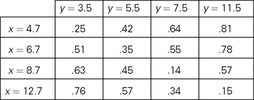
The RM principle was proposed in Dzhafarov (2002b) together with the related notion of an observation area. Note that x and y stimuli being compared belong to different sets, X and Y. This reflects the difference between two observation areas: even if x and y have the same value (say, they are line segments of the same length), they must occupy different spatial and/or temporal positions to be perceived as two distinct stimuli (see, e.g., Dzhafarov and Colonius, 2006). So x and y should be designated as, say, x = (5 cm, left) and y = (5 cm, right), and with this rigorous designation X and Y cannot even overlap. Moreover, even the values of the elements of X and Y (ignoring the difference in the observation areas) need not be the same. Thus, in the probability matrix below RM is satisfied in the simplest form (the minima on the main diagonal) even though the values of the stimuli in the first observation area (rows) and in the second one (columns) are not the same:

The distinction between two observation areas should be kept in mind for a correct application of the symmetry requirement, [C]. If in the statement “y matches x” the stimuli x and y exchange places, their values do so together with their respective observation areas. Thus, if the two observation areas are designated as “presented first” and “presented second” (chronologically within a trial), then the requirement [C] should be read as

[C, special case] if y, presented second, matches x, presented first, then x, presented first, matches y, presented second,

and not as

[C-look-alike, garbled] if y, presented second, matches x, presented first, then x, presented second, matches y, presented first.

In the latter statement, the pair (x, y) in the antecedent is different from the pair (x, y) in the consequent, creating thereby a confusion. A corrected version of [C-look-alike, garbled] could be

[C-look-alike, corrected] if a stimulus with value v₂ when presented second matches a stimulus with value v₁ presented first, then the stimulus with value v₁ when presented second matches the stimulus with value v₂ presented first.

Unlike [C-look-alike, garbled] this statement makes sense, but it is generally empirically false due to what is known as time-order error (more generally, constant error, see Dzhafarov and Colonius, 2006). By contrast, there seems to be no empirical evidence against [C, special case] or any other form of [C], which makes it possible to propose RM as a fundamental principle of pairwise comparisons (Dzhafarov, 2002b).

The notion of RM has been elaborated in Dzhafarov (2003), Dzhafarov and Colonius (2006), and Kujala and Dzhafarov (2008, 2009). It turns out to have nontrivial consequences for a variety of issues of traditional importance, ranging from Thurstonian-type modeling (see, e.g., Dzhafarov, 2006, in response to Ennis, 2006) to the “probability-distance” hypothesis (Dzhafarov, 2002a) to Fechnerian Scaling (see, e.g., Dzhafarov and Colonius, 2007) to matching-by-adjustment procedures (Dzhafarov and Perry, 2010) to the comparative version of the ancient “sorites” paradox (Dzhafarov and Dzhafarov, 2010a,b). In the latter two references the notion of RM (under the more general designation of “regular well-matched stimulus space”) was extended to an arbitrary set of observations areas. In the present work, however, we do not need to go beyond two fixed observation areas.

2. Regular Minimality for Rank Order Matrices Without Ties

In this paper we deal with the case when the stimulus sets are finite,

X = {x₁,…,x_n}, Y = {y₁,…,y_n},

and the discrimination function m(x, y) can be viewed as a matrix M = {m_ij}, i, j ∈ {1,…,n}. Clearly, a matrix which is not square cannot comply with RM (because each x has a unique y-match for which x is a unique match, and vice versa).

Convention 2.1. Henceforth we will assume that every matrix, unless otherwise specified, has pairwise distinct entries (contains no tied entries).

With this convention, the properties [A] and [B] are satisfied trivially (every row and every column has a unique minimal entry), and RM is reduced to the property [C] which now acquires the form

[RM = C] an entry is minimal in its column if it is minimal in its row.

The “column” and “row” in this statement can be exchanged and the statement above strengthened.

Lemma 2.2. In an RM-compliant matrix, an entry is minimal in its column if and only if it is minimal in its row.

Proof. To prove the “only if” part, let h be the mapping {1,…,n} → {1,…,n} defined by m_i,h(i) being the minimum entry in row i ∈ {1,…,n}. This mapping is injective, because if there were some rows i ≠ i′ with h(i) = h(i′), then m_ij would be the minimum entry in row i, m_i′j the minimum entry in row i′, whence the column h(i) would have to have two minimum entries. Since an injection {1,…,n} → {1,…,n} is also surjective, it follows that for every column j, is the minimum entry in both the row h⁻¹(j) and the column j, and the statement of the lemma follows from the uniqueness of this minimum value. ☐

In this paper we derive the formula for the proportion of RM-compliant matrices among all matrices with a given set of (pairwise distinct) entries. In other words, given any set V of n² distinct values of a discriminability measure (real numbers), we consider all n²! ways of placing these values in n² cells of an n × n matrix and count the number of matrices which are RM-compliant. The result is, obviously, invariant with respect to the set V. With no loss of generality, therefore we can assume that the matrices are filled with integers {1,…,n²} representing the ordinal positions of the elements of any possible set V. We will refer to these integer-valued matrices as rank order matrices (without ties), and their elements will be referred to as ranks.

Definition 2.3. A rank order matrix M is said to represent a matrix M′ (of the same size) if m_ij < m_i′j′ in M implies in M′, for any two cells (i, j) and (i′, j′).

Remark 2.4. Due to the bijective correspondence between the entries of M and M′, the “if” in this definition can be replaced or complemented with “and only if.”

Intuitively, the proportion of RM-compliant matrices among all rank order matrices of a given size seems to be the answer to the question: how likely is it to obtain a matrix M (not necessarily a rank order one) satisfying RM “by chance”? To explicate this intuition, we can adopt the following “meta-probabilistic” view. Consider the entries of M not as data but as theoretical (population-level) values of a discriminability measure. Assuming that the possible values for m_ij (i, j ∈{1,…,n}) form a set of reals 𝕊 of a positive Lebesgue measure (e.g., the interval [0, 1], as in the case when the m_ij’s are probabilities) we can impose on 𝕊 in each cell of the matrix some probability measure. Then we can pose the question of what the product measure is of the volume occupied by the RM-compliant matrices in . If one and the same measure μ is imposed on all entries, then all permutations of any given set of entries are equiprobable. The absence of ties among the entries in this approach is ensured by additionally assuming that the probability measure imposed is absolutely continuous with respect to the Lebesgue measure.¹ It is intuitively clear (and shown formally in the lemma below) that the product measure in question equals the proportion of the RM-compliant matrices among all possible rank order matrices. We will denote the product measure μ × … × μ (n² times) by .

Lemma 2.5. Let μ be a probability measure imposed on the set 𝕊 of a positive Lebesgue measure in each cell of an n × n matrix. Let μ be absolutely continuous with respect to the Lebesgue measure. Then the set of RM-compliant matrices in is -measurable and its -measure equals the proportion of RM-compliant matrices among all n × n rank order matrices (without ties).

Proof. Since 𝕊 is measurable, so is 𝕊 ∩]x, ∞[ for any real x, and so is

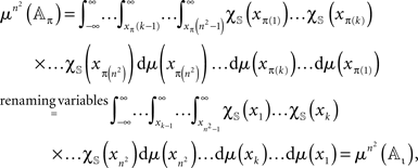
for any permutation π of (1,…,n²). The -measure of 𝔸_π is invariant with respect to π, which is obvious from symmetry considerations, or from the computation

where χ_𝕊(x) is the indicator function of 𝕊 on reals and ι the identity permutation. The Lebesgue measure of

is zero as this set lies within a finite union of (n² − 1) -dimensional hyperplanes. By absolute continuity of μ, Since

we have

whence for any π. Now, let π_RM be the set of all permutations represented by RM-compliant rank order n × n matrices, and let the number of these matrices be S_n. Then

which proves the lemma. ☐

Obviously, the theoretical values of a discriminability measure (such as probabilities of the response “different”) are not random variables. The measure μ imposed on 𝕊 therefore cannot be interpreted in frequency-related terms. Rather it can be thought of as a distribution of “subjective beliefs.” The assignment of one and the same measure μ to all cells then can be interpreted as a lack of subjective expectations with respect to possible associations between rows and columns. One cannot simply replace theoretical entries in this “meta-probabilistic” interpretation with data and treat μ as representing a hypothetical random variable. For one thing, if the possible set of data points is finite, as it is usually the case, this reinterpretation would necessitate finding a way of dealing with ties, as their probability would then no longer be zero. Most importantly, however, the null hypothesis that all cells of a matrix are generated according to one and the same distribution seems neither justified nor interesting. In another paper (Dzhafarov et al., 2010 under review), we propose both a simple way of dealing with tied entries and a data-analytic interpretation of the proportions of matrices with different degrees of RM-compliance, appropriately defined.

3. Proportion of RM-Compliant Matrices

Convention 3.1. Unless otherwise specified, henceforth every matrix mentioned will be assumed to be a rank order matrix (with no ties, in accordance with Convention 2.1).

Lemma 3.2. Let M_αβ be a matrix obtained from a matrix M by permutations α and β of its rows and columns, respectively. Then M_αβ = M_α′β′ implies (α, β) = (α′, β′).

Proof. Denoting M_αβ = M_α′β′ = M′, the entries m_ij and of M and M′, respectively, are related to each other as

and

If (α, β) ≠ (α′, β′) then, for some (i, j), and would have to be two identical entries in different cells, which is excluded by Convention 2.1. ☐

Lemma 3.3. If a matrix M satisfies RM, then so will any matrix M′ obtained from M by an arbitrary permutation of its rows and columns.

Proof. By arbitrary permutations α and β of the rows and columns, respectively, we transform M into a matrix M′. Its entries are related to the entries m_ij of M as

If m_ij in M is the minimum entry in the row i, then in M′ is the minimum entry in the row α(i), as the latter is merely the β-permutation of the row i of M; and if m_ij in M is the minimum entry in the column j, then in M’ is the minimum entry in the column β(j), as the latter is merely the α-permutation of the column j of M. Since permutations are bijective, it follows that the minimum entry in every row (column) in M′ is also the minimum entry in its column (respectively, row). ☐

Lemma 3.4. By appropriately chosen permutations of rows and columns one can bring any RM-compliant matrix M to a special form M′, in which the row and column minima are located on the main diagonal in the increasing order, This special form is unique for every M.

Proof. Let i₁,…,i_n be the rows of M arranged in the increasing order of their minima. Let these minima be located in the columns j₁,…,j_n, respectively. Then the permutations

and

are easily seen to yield M′ with the desired properties. The uniqueness statement follows from the uniqueness of the sequences i₁,…,i_n and j₁,…,j_n. ☐

The procedure is illustrated on the 4 × 4 RM-compliant matrix below, using the permutation of rows α = {1 → 3,2 → 2,3 → 1,4 → 4} and the permutation of columns β = {1 → 1,2 → 4,3 → 2,4 → 3}:

Definition 3.5. Let us refer to RM-compliant matrices in this special form (minima on the diagonal in increasing order) as special matrices.

Lemma 3.6. Denoting by s_n the number of n × n special matrices and by S_n the total number of n × n matrices satisfying RM,

Proof. Any matrix M that can be transformed (in the sense of Lemma 3.4) to a given special matrix M′ can be obtained from this M′ by means of permutations

and

The number of permutations α⁻¹ is n! and so is the number of permutations β⁻¹. Since every combination of α⁻¹ and β⁻¹ yields a unique matrix M (by Lemma 3.2), the number of such matrices for a given M′ is (n!)². The statement of the lemma follows. ☐

As an immediate consequence we obtain

Corollary 3.7. The proportion p_n of RM-compliant matrices among all n × n matrices is

☐

4. Main Theorem

We turn now to computing the number of RM-compliant matrices, S_n (n ≥ 1).

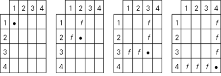
We will make use of the following notion. For k = 1,…,n, we will call the set of cells

in an n × n matrix M the kth frame (this set is empty for k = 1). Clearly, M is the union of its diagonal entries and its frames. The letters f in the 4 × 4 matrix below indicate its frame cells and the dots fill the corresponding diagonal cells:

Theorem 4.1. The number S_n of n × n RM-compliant matrices is

where

Remark 4.2. The combinatorial meaning of cmb(x,y) is the number of permutations of x objects taken y at a time (equivalently, the number of ways y distinct objects can be placed in x placeholders).

Proof. Let the diagonal entries (ranks) in the matrix M have been chosen and arranged as m₁₁ = d₁ < … < m_nn = d_n. We compute the number of ways in which we can fill the off-diagonal entries of M so that RM is satisfied in the special form (m_ij > d_i and m_ij > d_j if i ≠ j).

The nth frame should be filled by 2(n − 1) ranks chosen from the set of n² − d_n ranks exceeding d_n. The number of such choices is

None of these choices can violate the special form of RM, because any rank exceeding d_n will also exceed any d_k for k < n.

For k = 2,…,n − 1, let now all the frames above the kth have been filled without violating the special form of RM. The kth frame then should be filled by 2(k − 1) numbers chosen from the set of n² − d_k numbers exceeding d_k, from which however we should remove all the n² − k² numbers used up to fill in the previous n − k frames and diagonal elements. That is, the kth frame can be filled in by (n² − d_k) − (n² − k²) = k² − d_k numbers taken 2(k − 1) at a time. The number of such choices is

None of these choices can violate the special form of RM, because any rank exceeding d_k will also exceed any d_k′ for k′ < k, and if k′ > k then the choice above is irrelevant. The formula also applies to k = 1, since d₁ = 1 (any other placement of 1, the smallest rank in M, would violate RM), and cmb(1 − 1, 2 (1 − 1)) = 1, which is the number of ways to fill the empty first frame.

Since, for any given n-tuple d₁ < d₂ < … < d_n and any k = 1,…,n − 1, the value of cmb(k² − d_k, 2(k − 1)) does not depend on the fillings of the previous n − k frames, the number of ways of filling all n frames of M is

Then the number of special matrices is

and the statement of the theorem follows by Lemma 3.6. ☐

5. Computational Algorithm

Here we present the formula of Theorem 4.1 in a form which is less compact but more economic for computational purposes.

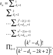
For every diagonal element d_k we have d_k ≥ d_k−1 + 1 if k > 1 (and d₁ ≥ 1); and in order for the multiplicands cmb(k² − d_k, 2(k− 1)) to be nonzero we should also require that d_k ≤ k² − 2(k − 1) for k = 1,…,n. It is easy to see, in particular, that the only values for the ranks d₂ and d₁ which satisfy these inequalities are 2 and 1, respectively. The formula for the number of special matrices acquires the form

The number of the arithmetic operations can be further reduced if we rewrite this as

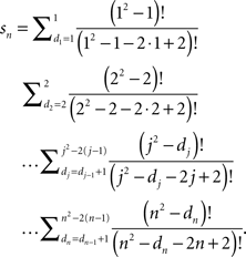
Algorithm 5.1. The following is a Mathematica™ program for computing precise values of p_n:

In[1]:=
cmb[a_, b_] := a!/(a - b)!;
up[c_] := c^2 - 2*c + 2;
F[n_, d_, k_] := F[n, d, k] = If[k < n,
   cmb[k^2 - d, 2*k - 2]* Sum[F[n, d1, k +
    1], {d1, d + 1, up[k + 1]}]];
F[n_, d_, n_] := cmb[n^2 - d, 2*n - 2]
In[2]:=
n = ???; (* ??? to be replaced with the
    desired value of n *)
Print[F[n, 1, 1]*(n!)^2/(n^2)!]

We present the values of p_n for n = 2,…,13, rounded to the sixth decimal place:

Under our “meta-probabilistic” interpretation, the table shows that the compliance with RM even for matrices as small as 4 × 4 or 5 × 5 can be considered “unlikely to occur by chance alone.”

Conflict of Interest Statement

The authors declare that the research was conducted in the absence of any commercial or financial relationships that could be construed as a potential conflict of interest.

Acknowledgments

This research has been supported by NSF grant SES 0620446 and AFOSR grant FA9550-09-1-0252 to Purdue University.

Footnote

1. ^Recall that a measure μ is absolutely continuous with respect to the Lebesgue measure if it is defined on the same sigma algebra, and if the m-measure of a set is zero whenever its Lebesgue measure is zero.

References

Dzhafarov, E. N. (2002a). Multidimensional Fechnerian scaling: probability-distance hypothesis. J. Math. Psychol. 46, 352–374.

CrossRef Full Text

Dzhafarov, E. N. (2002b). Multidimensional Fechnerian scaling: pairwise comparisons, regular minimality, and nonconstant self-similarity. J. Math. Psychol. 46, 583–608.

CrossRef Full Text

Dzhafarov, E. N. (2003). Thurstonian-type representations for “same-different” discriminations: deterministic decisions and independent images. J. Math. Psychol. 47, 208–228.

Dzhafarov, E. N. (2006). On the law of Regular Minimality: reply to Ennis. J. Math. Psychol. 50, 74–93.

Dzhafarov, E. N., and Colonius, H. (2006). “Regular Minimality: a fundamental law of discrimination,” in Measurement and Representation of Sensations, eds H. Colonius and E. N. Dzhafarov (Mahwah, NJ: Erlbaum), 1–46.

CrossRef Full Text

Dzhafarov, E. N., and Colonius, H. (2007). Dissimilarity cumulation theory and subjective metrics. J. Math. Psychol. 51, 290–304.

Dzhafarov, E. N., and Dzhafarov, D. D. (2010a). Sorites without vagueness II: comparative sorites. Theoria. 76, 25–53.

CrossRef Full Text

Dzhafarov, E. N., and Dzhafarov, D. D. (2010b). “The sorites paradox: a behavioral approach,” in Mathematical Models for Research on Cultural Dynamics: Qualitative Mathematics for the Social Sciences, eds J. Valsiner and L. Rudolph (Routledge: London), in press.

Dzhafarov, E. N., and Perry, L. (2010). Matching by adjustment: if X matches Y, does Y match X? Front. Quant. Psychol. Meas. 4: 24, 1–16. doi: 10.3389/fpsyg.2010.00024.

Ennis, D. M. (2006). Sources and influence of perceptual variance: comment on Dzhafarov’s Regular Minimality principle. J. Math. Psychol. 50, 66–73.

Kujala, J. V., and Dzhafarov, E. N. (2008). On minima of discrimination functions. J. Math. Psychol. 52, 116–127.

Kujala, J. V., and Dzhafarov, E. N. (2009). Regular Minimality and Thurstonian-type modeling. J. Math. Psychol. 53, 486–501.