Matching by adjustment: if X matches Y, does Y match X?

When dealing with pairwise comparisons of stimuli in two fixed observation areas (e.g., one stimulus on the left, one on the right), we say that the stimulus space is regular well-matched if (1) every stimulus is matched by some stimulus in another observation area, and this matching stimulus is determined uniquely up to matching equivalence (two stimuli being equivalent if they always match or do not match any stimulus together); and (2) if a stimulus is matched by another stimulus then it matches it. The regular well-matchedness property has non-trivial consequences for several issues, ranging from the ancient “sorites” paradox to “probability-distance hypothesis” to modeling of discrimination probabilities by means of Thurstonian-type models. We have tested the regular well-matchedness hypothesis for locations of two dots within two side-by-side circles, and for two side-by-side “flower-like” shapes obtained by superposition of two cosine waves with fixed frequencies in polar coordinates. In the location experiment the two coordinates of the dot in one circle were adjusted to match the location of the dot in another circle. In the shape experiment the two cosine amplitudes of one shape were adjusted to match the other shape. The adjustments on the left and on the right alternated in long series according to the “ping-pong” matching scheme developed in Dzhafarov (2006b, J. Math. Psychol., 50, 74–93). The results have been found to be in a good agreement with the regular well-matchedness hypothesis.

1. Introduction

Consider a description of an experiment in which two stimuli were visually presented side-by-side. Let the description say, in part, that

a participant adjusted the color [or intensity, or shape] of a stimulus on the right until the appearance of this stimulus matched the appearance of the stimulus on the left.

The author of this quote would not probably hesitate to rewrite it as

a participant adjusted the color [or intensity, or shape] of a stimulus on the right until the appearance of this stimulus was matched by the appearance of the stimulus on the left.

Or

a participant adjusted the color [or intensity, or shape] of a stimulus on the right until the appearance of this stimulus and the appearance of the stimulus on the left matched each other.

Note that we are not dealing here with differently formulated instructions to a participant, nor with different procedures of adjustment. Rather we have three “theoretical” descriptions of a certain performance (under a given instruction and by a given procedure), and these three descriptions appear interchangeable. This theoretical belief is likely to be shared by the participants in such an experiment themselves: if a participant declares “I think that now this right shape matches this left one,” then the questions like “And do you also think that the left one matches the right one?” or “Do you also think they both match each other?” are likely to be met by a questioning stare.

This simple observation leads us to propose that a valid theoretical definition of the notion “stimulus y matches stimulus x”¹ should be constructed so that the relation it depicts be symmetric:

Note that if x and y in the relation “y matches x” are, say, the left and the right stimuli, respectively (and so the relation in question means that the right stimulus matches the left one in some property or overall, but ignoring the conspicuous difference in locations), then they retain these locations in the relation “x matches y.” So, the statement in (1) for left–right stimuli should be read as

y (on the right) matches x (on the left)

if and only if

x (on the left) matches y (on the right).

Analogously, if x and y in the relation “y matches x” are presented in a temporal succession, x first, y second, then (1) means

y (second) matches x (first)

if and only if

x (first) matches y (second),

and not (contrary to a common procedural mistake)²

y (second) matches x (first)

if and only if

x (second) matches y (first).

The latter statement is generally wrong due to the presence of constant error (here, time order effect).

Our goal in this paper is to construct a definition of matching and to experimentally test its compliance with the symmetry requirement (1) for the matching-by-adjustment paradigm. Given our opening example, one might wonder why we need a theoretical definition of matching in the first place. Why cannot we simply say that stimulus y matches stimulus x when an observer says so? The reason is that pairwise comparisons are probabilistic: one cannot say “y is judged to be the same as x” without adding “in this trial” (and then in another trial this may not be true) or “with this probability” (and then another stimulus y′ will be judged to be the same as x with some other probability). As a result, the identity of a stimulus y matching x has to be computed from a set of responses rather than observed in a single one.

To make this clear, consider the classical paradigm of greater–less comparisons. Let us say x is the stimulus presented on the left, y is presented on the right, and in response to a left–right pair (x,y) a participant says which of the two contains more of a certain property (say, brightness). The participant is not allowed to say that the two stimuli are equally bright, so one could not identify the matching relation with the participant’s judgments even if they were deterministic. The fact is, however, they are probabilistic, and each pair of stimuli maps into a probability with which the right stimulus is judged to be greater (in brightness) than the left one,

If we view this function as , with x fixed, then the match (or point of subjective equality, PSE) for x is traditionally defined as any value of y (may not be unique if y is not unidimensional)³ for which ξ(x,y) = 1/2. Viewing the function as , with y fixed, the match (or PSE) for y is analogously defined as any value of x at which ξ(x,y) = 1/2. It is easy to see that with this definition of matching, y matches x if and only if x matches y.

The symmetry of the matching relation, however, is not always a mathematical necessity. With other definitions of matching it may be an empirical hypothesis. Nor is this hypothesis always innocuous and trivial. It often has in fact unexpectedly restrictive consequences. To see this, consider the paradigm of same–different comparisons. Let stimuli x,y, again, be presented on the left and on the right, respectively, and let a participant say in response to a pair (x,y) whether the two stimuli are different (in some respect, such as brightness, or overall). Each stimulus pair now is associated with the probability

A natural definition of a match (PSE) for x here is any value of y such that ψ(x,y) is the smallest value of the function Analogously, any value of x at which the function achieves its minimum value is taken to be a match (PSE) for y. With this definition of matching it is no longer obvious that y matches x if and only if x matches y. In fact, it is very easy to construct models that would be incompatible with this statement. This is true, in particular, for Thurstonian-type models, a widely used theoretical tool about which Luce (1977, p. 462) said that “this conception of internal representation of signals is so simple and so intuitively compelling that no one ever really manages to escape from it.”

Consider the simplest such a model, proposed in Luce and Galanter (1963). Stimuli x and y in this model are mapped into independent univariate normal random variables R_x and R_y, and the response “same” is given if and only if |R_x − R_y| is less than some fixed constant. Suppose that the variances and are continuously differentiable functions of the corresponding means, Since in this case any two x-values that map into an R_x with a given mean, hence also a given variance, are equivalent (i.e., they match or do not match any stimulus y together), and analogously for y-values, we can conveniently speak of “stimuli μ_x and μ_y” in place of x and y.⁴ Assuming that μ_x and μ_y fill in respective intervals of reals, it can easily be shown (Dzhafarov, 2003a, 2006b) that there are some functions H and G such that (A) any stimulus μ_x is matched by a single μ_y = H(μ_x), (B) any stimulus μ_y is matched by a single μ_x = G(μ_y), but (C) G is not the inverse of H unless the variances and have constant values. In other words, if and in this model change with stimuli, then the PSE of the PSE of a given stimulus (μ_x or μ_y) is generally different from this stimulus. One can show that this situation cannot be “corrected” by replacing the independent univariate normal distributions in this model with more complex and stochastically interdependent distributions on other probability spaces (provided that the model remains “well-behaved” in some rather non-restrictive sense; see Dzhafarov, 2003a,b, 2006a, and Kujala and Dzhafarov, 2009). We see that the requirement that y match x if and only if x matches y is far from being innocuous: it imposes rather stringent constraints on the possible Thurstonian-type models (see Dzhafarov, 2006b, in response to Ennis, 2006).

Another modeling scheme for which the requirement in question is critical is the “probability-distance hypothesis” (Dzhafarov, 2002a). In this class of models, assuming that both x and y stimuli (say, presented on the left and on the right, respectively) take their values in some common set ӡ, the probability with which x and y are judged to be different is an increasing function Φ of some metric D imposed on ӡ:

Although traditionally applied to greater–less rather than same–different judgments, this modeling scheme pertains to what Luce and Edwards (1958, p. 232) called “the old, famous psychological rule of thumb: equally often noticed differences are equal.” Now, a direct application of (4) implies that achieves its minimum (i.e., y matches x) if and only if y = x; and that achieves its minimum (i.e., x matches y) if and only if x = y. The symmetry requirement therefore must be satisfied in order for the model to hold. A more sophisticated approach takes into account the possibility of constant error (non-coincidence of the values of a stimulus and its PSE) and modifies (4) as

ψ(x,y) = Φ[D(H(x),y)],

where H is some bijective function. It is easy to see that both and achieve their (common) minimum if and only if y = H(x), ensuring thereby that y matches x if and only if x matches y.

Yet another issue in which the symmetry in question plays an important role is known in philosophy as the perceptual variety of the “sorites paradox” (see, e.g., the collections of chapters edited by Keefe and Smith, 1999; Beall, 2003). In both philosophy and psychophysics the issue is also known as that of nontransitivity of matches (Goodman, 1951/1997; Luce, 1956). Somewhat simplifying, let the matching y for x be determined uniquely, y = H(x), and let the matching x for y be determined uniquely as well, x = G(y). Then the PSE for y = H(x) is x′ = G ○ H(x). If G is not the inverse of H, x′ does not generally coincide with x. The PSE for x′ in turn is y′ = H ○ G ○ H(x), which does not generally coincide with y and therefore does not match the initial value of x. We obtain thus a “tetradic soritical sequence” (Dzhafarov and Dzhafarov, 2010b)

This situation does not occur if matches are symmetric, G ≡ H⁻¹. Then x′ = x and y′ = y, that is, the last element of the sequence, y′, matches its first element, x.⁵

It should be mentioned, to prevent misunderstandings, that the possibility or impossibility of soritical sequences is determined not only by the issue of symmetry of matches but also by that of their uniqueness. Thus, many authors take it for granted that if y matches x then any y* which is sufficiently close to y will also match x. This position, however, is logically untenable as it leads to a contradiction (see Dzhafarov and Dzhafarov, 2010a, for a detailed analysis). Not to discuss this on a general level, let matching be determined through the function ξ(x,y) in (2), and let the stimulus values be unidimensional, which we indicate by using the notation x = x, y = y. Let (x,y) be a left–right pair of matching stimuli, which we know to mean that ξ(x,y) = 1/2. It would be fallacious now to maintain that whenever this happens, ξ(x,y + ε) must remain equal to 1/2 for sufficiently small |ε| – such an assertion would in fact imply that the function equals 1/2 over all values of y. If the latter is not the case, then there must be at least one value of y matching x such that no value y* to the right and/or to the left from y matches x, however close to y. It is reasonable to assume in fact, as it is done in all models and fits of psychometric functions known to us from the literature, that the value of y (or x) for which ξ(x,y) = 1/2 is unique for all x (respectively, y) – because with conventional choices of stimulus continua is strictly increasing in the vicinity of its median (respectively, is strictly decreasing in the vicinity of its median). Even if we speculate, with no empirical justification, that in some cases the function may have a plateau at the level 1/2 over some interval ]y − ε, y + ε[, it is reasonable to assume then (in the absence of any empirical evidence to the contrary and in accordance with the regular well-matchedness hypothesis formulated in Section 2) that any two y₁,y₂ stimuli in this interval are equivalent: ξ(x,y₁) = ξ(x,y₂) for all x.

Let us return now to our opening example: two stimuli, one of them fixed, the other manipulated by a person until it appears matching the fixed one. A mapping of some physical process (such as trackball rotation) into a set of stimuli normally requires a parametrization of stimuli by reals, so we may assume that x and y are vectors of reals. If we imagine the adjustment procedure repeated infinitely many times under the same conditions, each fixed stimulus, x or y, will correspond to a random variable Y_x with y-values (respectively, a random variable X_y with x-values). How should one define the matching stimulus (PSE) for x or y in this situation? The traditional answer is to take some measure of central tendency of Y_x and X_y, such as their expected values or componentwise medians. One needs, however, a theory that would justify suitable choices for this measure. Most important in the present context, given different choices one should opt for those that ensure (or at least make it plausible) that the matching relation is symmetric: denoting a measure of central tendency by m,

This consideration makes it clear that a suitable definition of the PSE for x or y has to be tied to a particular parameterization of stimuli. Indeed, with no conventional choice of m, if (6) holds for x and y will it also hold for x′ = T₁(x) and y′ = T₂(y) across all possible reparametrizations T₁,T₂, even if one confines the latter, as we do in this paper, to diffeomorphisms only (continuously differentiable bijections with continuously differentiable inverses).

2. An Approach to Matching by Adjustment

2.1. Regular Well-Matchedness

The general notion of a regular well-matched stimulus space has been developed in Dzhafarov and Dzhafarov (2010b) for an arbitrary set of stimuli and observation areas (defined, e.g., by multiple locations of stimuli compared in shape, or multiple colors of stimuli compared in brightness). For detailed discussions of the notion of an observation area and its importance in the theory of comparative judgments see Dzhafarov (2002b), Dzhafarov and Colonius (2006), and Dzhafarov and Dzhafarov (2010b). Here we confine our consideration to the case when stimuli belong to two fixed observation areas. Let us agree to use letters x and a to denote stimulus values in the one of them (say, left, or first), and letters y and b to denote stimulus values in the other (right, second). More rigorous notation would be (x, 1) or x⁽¹⁾, meaning the stimulus with value x in observation area 1, and analogously for y, but the simplified notation seems sufficient in the present context.

Let us assume that the set of all x and y stimuli is endowed with a binary relation M (“is matched by”) which can only hold true for two stimuli from different observation areas: xMy or yMx but never x₁Mx₂ or y₁My₂. Let us also define a binary relation E (“is equivalent to”) which, on the contrary, only holds for two stimuli from one and the same observation area: x₁Ex₂ means that for any y, yMx₁ ⇔ yMx₂; analogously, y₁Ey₂ means that for any x, xMy₁ ⇔ xMy₂.

We say that the x and y stimuli form a regular well-matched space if they satisfy the following statements:

𝒲ℳ (well-matchedness property). For any stimulus (x or y) there is a stimulus in another observation area (respectively, y or x) such that the two stimuli match each other (xMy and yMx).

ℛ (regularity property). If two stimuli in the same observation area (x₁,x₂ or y₁,y₂), are matched by another stimulus (respectively, y or x), then they are equivalent (x₁Ex₂, or y₁Ey₂, respectively).

The requirement of regular well-matchedness is all one needs to ensure that matching is “non-paradoxical”: no possibility for nontransitive sequences like (5), and no violations of symmetry (1). It is convenient in the present context to reformulate the definition of a regular well-matched space of stimuli in the form maximally emphasizing the symmetry property. Assume that all x and y stimuli have been (re)labeled so that any two equivalent stimuli receive one and the same label. Retaining the same notation (x and y) for thus (re)labeled stimuli, no two different x (or y) stimuli are equivalent. With this proviso, the stimuli form a regular well-matched space if the following statements hold:

ℳℱ (matching is a function). For every stimulus there is one and only one stimulus in the other observation area which matches it; that is, there is a function H such that xMy ⇔ y = H(x), and a function G such that yMx ⇔ x = G(y).

ℳ𝒮 (matching is symmetric). For any x, y, yMx ⇔ xMy.

The equivalence of ℳℱ–ℳ𝒮to 𝒲ℳ–ℛ is obvious. The functions H and G are referred to as PSE functions, with H(x) being the PSE for x and G(y) the PSE for y. Once ℳℱ is accepted, the property ℳ𝒮 says that the functions H and G are bijective and each other’s inverses: G ≡ H⁻¹. This formulation is close to the definitions of Regular Minimality and Regular Mediality given in Dzhafarov (2003a) and Dzhafarov and Colonius (2006) for, respectively, same–different and greater–less comparisons (the formulation in Dzhafarov and Dzhafarov, 2010b, is better suited for multiple observation areas).

The reason ℳℱ–ℳ𝒮 is more convenient for our purposes than 𝒲ℳ–ℛ is that it is usually easy to construct a definition of matching that satisfies ℳℱ, and whenever this is the case (as it is, e.g., in the Luce–Galanter model mentioned in Section 1), the question of whether a stimulus space is regular well-matched reduces to the title question of this paper. Most importantly in the present context, ℳℱ is trivially satisfied for the matching-by-adjustment paradigm: if each x corresponds to a one and only one random variable Y_x (with values representing declared y-matches to x in different trials), then any measure of central tendency m[Y_x] is a function of x, m[Y_x] = H(x); and analogously with y and m[X_y] = G(y). The question is whether m can be chosen so that G ≡ H⁻¹. Figure 1 illustrates three situations of interest: when ℳ𝒮 is violated, when it is satisfied, and when ℳ𝒮 it is violated but it is difficult if not hopeless to distinguish it from the case of compliance with ℳ𝒮 in a realistic experiment. With an appropriately formulated general model the situations illustrated in the left-hand and middle panels of the figure can be made sources for competing statistical hypotheses.

FIGURE 1

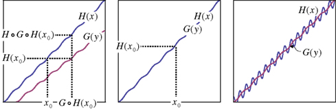
Figure 1. x and y stimuli (for illustration purposes unidimensional) with the PSE functions H(x) and G(y). The abscissa segment and ordinate segment depict “sufficiently large” areas of stimuli around x₀ and y₀ = H(x₀), respectively. Left-hand panel: the symmetry assumption, ℳ𝒮, is not satisfied, and the two functions do not cross within the areas depicted. Middle panel: ℳ𝒮 is satisfied. Right-hand panel: ℳ𝒮 is not satisfied but the two functions have numerous crossings within the areas depicted. In the left-hand panel the PSE for the PSE of x₀ is not x₀ itself, and analogously for y₀ = H(x₀): there are systematic differences between G ○ H(x₀) and x₀, and between H(x₀) and H ○ G ○ H(x₀) which may be detectable if the procedure is repeated many times and the errors of matching are sufficiently well-behaved. In the middle panel the PSE for the PSE of x₀ is x₀ itself, and analogously for y₀ = H(x₀): if the procedure is repeated many times any variance among successive adjustments of x and y will be due to matching errors only.

2.2. General Model

The general model in question is as follows. Let the values of x and y (after equivalent stimuli have been identically labeled) be representable by real-valued vectors, x = (x¹,…, xⁿ), y = (y¹,…,yⁿ), filling in two open connected areas of ℝⁿ.⁶ Let the random vectors Y_x and X_y be as defined above. We assume the existence of two diffeomorphic transformations, x = T₁(a) and y = T₂(b), with each of a and b filling in ℝⁿ, such that

where h and g are continuously differentiable functions, and (δa, δb) is a 2n-vector of independent normally distributed variables with zero means⁷. We define the PSE functions for, respectively, x = T₁(a) and y = T₂(b) as the continuously differentiable functions

In our general notation,

Note that this definition of the PSE functions H and G does not tell us how to compute them from Y_x and X_y, respectively, as our general model does not specify the transformations T₁,T₂. We will be able to circumvent this difficulty in the application of the model to our experiments (in Section 3.1) by using linear approximations to T₁ and T₂. In Section 7 we mention an approach which may make the reliance on approximations unnecessary. This issue is related to the uniqueness properties of T₁,T₂, which is worth mentioning even if not essential for the analysis to follow.

Clearly, if T₁, T₂ exist, then T₁ ° L₁, T₂ ° L₂ will be another pair of transformations providing (7), for any choice of orthogonal linear transformations L₁, L₂. Linear transformations, however, are inconsequential, as they do not change the PSE functions H and G. If x,y belong to ℝ¹ or ℝ² (arguably the most important cases amenable to experimental analysis), then it is known that within a class of transformations including diffeomorphisms (under certain constraints trivially satisfied in our general model), linear transformations are the only ones which preserve the normality of δa and δb (Ghosh, 1969; Khatri and Mukerjee, 1987). In other words, for univariate and bivariate stimuli the PSE functions in the general model are determined uniquely. There are reasons to conjecture (Khatri, 1987) that this is also true for n > 2, but the results we know of are less general than for n = 1, 2. There does not, however, seem to be a known example of a nonlinear diffeomorphism in ℝⁿ that would map n + 1 normal distributions with distinct means into n + 1 normal distributions with distinct means.

2.3. Null Model

We say “null model” instead of “null hypothesis” to emphasize that the former is an essentially non-statistical theoretical construct which may be used as a source of (generally more than one) statistically testable consequences, which then will be referred to as null hypotheses.

The null model is obtained from the general model by positing that h and g in (7) are diffeomorphisms, and

g ≡ H⁻¹.

It follows from (8) that

or (as illustrated in the middle panel of Figure 1)

G ≡ H⁻¹.

From (9) we have then

xMy if and only if yMx.

2.4. Alternative Model

The alternative model corresponds to the left-hand panel of Figure 1. Since its difference from the right-hand panel is a matter of scale only, the alternative model has to be formulated in reference to the set of stimuli recorded in a specific experiment (whether set by experimenter or adjusted by participant). Let {x₁,…,x_M} and {y₁,…,y_N} be these stimuli. Let us define a sufficiently large stimulus area for x as any open connected area 𝒳 of x-values that contains {x₁,…,x_M} ∪ {G(y₁),…,G(y_N)}, where G is the true PSE function for y as defined by (8) in the general model. Analogously, a sufficiently large stimulus area 𝒴 for y is any open connected area of y-values that contains {y₁,…,y_N} ∪ {H(x₁),…,H(x_M)}.

The alternative model says that in some sufficiently large areas 𝒳 and 𝒴 the graphs of the corresponding components of PSE functions H(x) and G(y) do not cross. This means that for any i = 1,…,n, the ith component of the difference H(x) − y has one and the same sign across all x ∈ 𝒳 and y ∈ 𝒴 such that H(x) ∈ 𝒴 and G(y) = x; analogously, for any i = 1,…,n, the ith component of the difference G(y) − x has one and the same sign across all y ∈ 𝒴 and x ∈ 𝒳 such that G(y) ∈ 𝒳 and H(x) = y.

3. Ping-Pong Matching Paradigm

If there was no matching error involved, then starting with any x ∈ 𝒳 one could create two sequences of stimuli, one in each observation area (let them be again “left” and “right”), chain-matched as shown in Figure 2. Under our alternative model, each stimulus in each observation area is different from the one immediately following it. Moreover, for any i = 1,…,n, the differences , etc., have one and the same sign, and so do the differences , etc., in the other observation area. If the null model is true, however, then (in the absence of matching errors) all x’s are the same and so are all y’s, whence all the componentwise differences between successive stimuli in either observation area are 0.

FIGURE 2

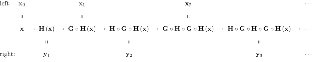
Figure 2. A chain-matched sequence of left and right stimuli. The arrows should be read “is matched by” (i.e., they represent the relation M).

The ping-pong matching paradigm proposed in Dzhafarov (2006b) is aimed at distinguishing between these two competing possibilities in the presence of matching errors. The logic of the paradigm is presented in Figure 3. As an example, in three ping-pong matching experiments reported in Dzhafarov (2006b), stimuli were straight line segments presented side-by-side in a frontal plane, and in each trial a participant had to adjust one of the segments until it appeared of the same length as the other one, held fixed. Every time a “balance point” was achieved, the balance was upset by randomly changing the length of the segment which was fixed in the previous trial, and the participant had to adjust it “back,” until it matched the length of the other segment (which remained fixed at its previously established value). This alternating procedure was replicated 200 times (100 balance points on each side), and each of these 200-trial series was repeated 10–25 times. In reference to Figure 3, x = x and y = y are unidimensional, so the first-order differences are Δx_k = x_k+1 − x_k and Δy_k = y_k+1 − y_k.

FIGURE 3

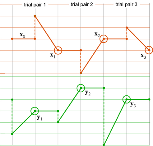
Figure 3. A schematic representation of ping-pong adjustments. The top and bottom panels correspond to two observation areas, the vertical axes representing stimulus values (which need not, however, be unidimensional). Trials may or may not be separated by time intervals. A series of adjustments consists of many consecutive trial pairs. In the first trial of any trial pair, x remains fixed (solid horizontal lines, top panel) at the value established at the end of the previous trial pair; the value of stimulus y at the beginning of this first trial is randomly offset (dashed vertical lines, bottom) so that it generally does not match x, and the participant adjusts this value (oblique solid lines, bottom) until it seems to match x (the encircled points, bottom); in the second trial of the trial pair, y remains fixed (solid horizontal lines, bottom) at the value established at the end of the previous trial; the value of stimulus x at the beginning of this second trial is randomly offset (dashed vertical lines, top) so that it generally does not match y, and the participant adjusts this value (oblique solid lines, top) until it seems to match y (the encircled points, top). The stimuli x₁,x₂,x₃,… and y₁,y₂,y₃,… represented by the encircled points are referred to as “balance points.” In this work we focus on the first-order differences Δx_k = x_k+1 − x_k and Δy_k = y_k+1 − y_k between balance points.

As shown below (Sections 3.1–3.3), to the extent one can drop non-linear terms in certain Taylor expansions, it follows from the null model that the distributions of the Δx_k and Δy_k should be symmetric around 0. The histograms and statistics shown in Figure 4 do not contradict this prediction.

FIGURE 4

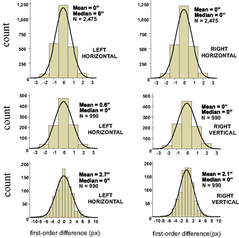
Figure 4. Histograms of first-order differences for ping-pong adjustments of line segments’ lengths. The data are shown for a single participant in three experiments: with two short horizontal lines on the left and on the right (top panel), and with a horizontal line on the left and a vertical line on the right (middle panel for short lines, bottom panel for longer lines). The abscissae are calibrated in screen pixels (1 px ≈ 55 sec arc). The means and medians are shown in sec arc. See the opening text of this section and Dzhafarov (2006b) for details.

Dzhafarov (2006b), however, does not offer a general model of matching-by-adjustment. Also, one can be skeptical about the generalizability of unidimensional results to multidimensional stimuli.⁸ The present work is to fill in these gaps. In the remainder of this section we show how the general model of Section 2 and its null and alternative versions apply to the ping-pong adjustment paradigm.

3.1. Application of the General Model

Let us enumerate the trial pairs (as described in the legend to Figure 3) 1,2,…,N, in chronological order. Denote the balance points established in the kth trial pair by (y_k,x_k) and the first-order differences (or Δ’s for short) by Δx_k = x_k+1 − x_k and Δy_k = y_k+1 − y_k. It is shown in the Appendix that the general model of Section 2 implies

where M…,N… denote n × n matrices, and o designates any function whose norm |o| (say, the supremal one) is o{1}|(δa₁,δb₁,…,δa_k+1,δb_k+1)|. We know that (δa_k,δb_k) is a 2n-vector normally distributed with zero mean and a diagonal variance matrix, for every k. Let us additionally assume that (δa_k,δb_k) and (δa_k′,δb_k′) are independent for any k ≠ k′. It follows then that to the extent one can ignore the o-terms, every component of Δy_k and every component of Δx_k are approximately normally distributed (i = 1,…,n). Note however that (Δx_k,Δy_k) and (Δx_k′,Δy_k′) for k ≠ k′ generally have different means and variances, and any two components of the 4n-vector (Δx_k,Δy_k,Δx_k′,Δy_k′) are generally stochastically interdependent. The sequences and therefore are not generally sequences of iid variables.

3.2. Null Hypotheses

The situation simplifies considerably under the null model. As shown in the Appendix, (10) then acquires the form

where the matrices M₁, M₂, N₁, N₂ are now fixed. To the extent one can ignore the o-terms, it follows that for i = 1,…,n, either of and is a sequence of iid variables normally distributed around 0 (although any two variables from with i ≠ j are generally interdependent). One can drop index k and speak of random variables

where (δa, δa′, δb) is a 3n-vector of independent normal variates with zero means. Since the smaller the values of |Δyⁱ| the more likely it is to correspond to small values of |δa|,|δa′|,|δb| in (12) and the better justified one is in dropping the o-terms, one should expect that for a sufficiently small εⁱ > 0, the values of Δyⁱ in the interval 0 ± εⁱ should be distributed symmetrically around zero; and the same should be true for Δxⁱ in an interval 0 ± єⁱ.

The choice of εⁱ and єⁱ, for i = 1,…,n, depends on the precision needed (which in turn depends on sample size) and on the test of symmetry one chooses to use (cruder tests allow for wider intervals). Thus, εⁱ and єⁱ may very well be chosen differently in the three null hypotheses we use to assess the compliance of the experiments reported below with the symmetry prediction of the null model.

H1₀: For some sequence ,

where m = 0,1,…,l_i − 1 and ; and an analogous statement is true for Δxⁱ and some partition

H2₀: The population mean of Δyⁱ-values falling between −εⁱ and εⁱ is 0; and the same is true for Δxⁱ between −єⁱ and єⁱ.

H3₀: The population median of Δyⁱ-values falling between −εⁱ and εⁱ is 0; and the same is true for Δxⁱ between −єⁱ and єⁱ.

In order not to bias the outcomes in favor of the nulls, in the analysis of our experiments we simply put ε = є = ∞, that is, we used the entire range of data. In H1₀, however, we could only choose narrow grouping bins and in a small vicinity of 0, lumping together more peripheral values. We used the same grouping scheme in all conditions of both our experiments.

3.3. Alternative Hypotheses

Under the alternative model, for any i = 1,…,n, the random variables in the sequence are neither identically distributed nor independent. But they are all distributed normally with the means , all positive or all negative. Let us denote this common sign of the ’s by sgn(vⁱ). By aggregating across all k we create a random variable Δyⁱ which equals with probability 1/N. Since for any positive numbers α < β,

we have

sgn(Pr[α ≤ Δyⁱ < β] − Pr[−β ≤ Δyⁱ < −α]) = sgn(vⁱ).

It follows that the conclusion we have drawn from the null model, that the values of Δyⁱ in some interval 0 ± εⁱ should be distributed symmetrically around 0, is false under the alternative model. In particular, sgn(Pr[0 ≤ Δyⁱ < εⁱ] − Pr[−εⁱ ≤ Δyⁱ < 0]) = sgn(vⁱ) whence the median of Δyⁱ in any interval 0 ± εⁱ (including for εⁱ = ∞) also shares the sign with vⁱ. The same is true about the mean Δyⁱ, which equals . The consideration of and their mixture Δxⁱ is analogous and leads to the same conclusions.

We can now formulate, for each i = 1,…,n and any choice of εⁱ,єⁱ, the alternative hypotheses corresponding to H1₀−H3₀ of the previous section.

H1_A: For any sequence chosen in H1₀, it is not true that

where m = 0,1,…,l_i − 1; and an analogous negative statement holds for Δxⁱ.⁹

H2_A: The population mean of Δyⁱ-values falling between any −εⁱ and εⁱ chosen in H2₀ is not 0; and analogously for Δxⁱ.

H3_A: The population median of Δyⁱ-values falling between −εⁱ and εⁱ chosen in H3₀ is not 0; and analogously for Δxⁱ.

We have mentioned in the previous section how we chose the intervals and partitions for the experiments reported below.

4. Materials and Methods

4.1. Participants

Seven paid volunteers, students at Purdue (six females and one male) and the second author of this paper (LP) served as participants in two experiments. The paid volunteers, naive as to the aims and designs of the experiments, are identified as P1–P3 (in the location experiment) and P4–P7 (in the shape experiment). LP participated in both experiments. All participants were aged around 20 and had normal or corrected to normal vision.

4.2. Stimuli and Procedure

The stimuli used are exemplified in Figure 5 and described in its legend, together with the observation conditions. In each trial a participant changed the parameters of one of the two stimuli by rotating a trackball on which the participant rested her/his dominant hand.

FIGURE 5

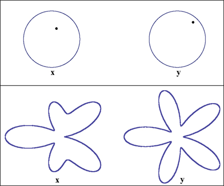
Figure 5. Stimuli used in the location experiment (top panel) and the shape experiment (bottom). In both experiments the two observation areas are defined as “left” and “right.” The two stimuli were displayed on a flat-panel monitor viewed (using a chin rest with forehead support) from the distance of 90 cm, making 1 screen pixel ≈ 62 sec arc. The stimuli were grayish-white on black, of a comfortably low fixed luminance, viewed in darkness. In the location experiment the stimulus values x on the left and y on the right are locations of the dots within their circles: they are measured by the horizontal and vertical Cartesian coordinates of the dots with respect to the circles’ centers. The width of the circumferences and the diameter of the dots in the experiment were 5 px, the circles’ radii measured 70 px, and the distance between the circles’ centers was 150 px. The initial value of x in the experiment was (27 px, 16 px), corresponding to (π/6, 0.45 radius) in polar coordinates. In the shape experiment the stimulus values x on the left and y on the right are the amplitudes A₃ and A₅ in the formula for a “floral” shape in polar coordinates: R + A₃cos3θ + A₅cos5θ, where |A₃| + |A₅| ≤ R. In the experiment R was 70 px, the distance between the floral shapes’ centers was 300 px, and the width of the contours 5 px. The initial value of x in this experiment was A₃ = A₅ = 0.2R = 14 px.

In the location experiment the horizontal and vertical rotations of the trackball controlled the horizontal (x¹ or y¹) and vertical (x² or y²) coordinates of one of the dots. Each trial began by the two circles with the dots appearing on the screen. In accordance with the logic of ping-pong adjustments (Figure 3), one of the dots was kept at the same location as established at the end of the previous trial [or, in trial 1, at the initial value (27 px, 16 px)], while the other dot at the beginning of the trial was at a randomly chosen location as shown in Figure 6. The participant was instructed to move this dot until its location matched that of the other, fixed dot, and to click a button on the trackball device when satisfied. With this click the trial ended and the two stimuli disappeared, to appear again 0.5 s later. Each series of ping-pong adjustments consisted of 100 trial pairs (100 y-adjustments in the odd-numbered trials and 100 x-adjustments in the even-numbered ones). There were two such series per participant per day, separated by a few minutes, each preceded by a practice series of 20 trial pairs (which was not recorded). In total each of the four participants worked through 20 ping-pong series. This amounted to the total of 2000 balance points for each of y¹, y², x¹, x², yielding 1980 values for each of the corresponding first-order differences.

FIGURE 6

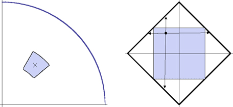
Figure 6. A detailed view of the adjustment procedure in the location (left) and shape (right) experiments. The left-hand picture shows the first quadrant of the circle in which the location of the dot is manipulated. The cross shows the location of the dot in the previous trial. Denoting its polar coordinates by (θ,r), at the beginning of the current trial the dot’s location is randomly chosen according to the uniform distribution over the rectangle (θ − π/18, θ + π/18) × (r − 0.1 radius, r + 0.1 radius) in polar coordinates (shown by the colored area). The right-hand picture shows the space of the A₃,A₅-amplitudes,|A₃| + |A₅| ≤ R, for the shape being adjusted. At the beginning of the current trial the values of A₃,A₅ (irrespective of their values in the previous trial) are randomly chosen according to the uniform distribution over the square (−0.5R, 0.5R) × (−0.5R, 0.5R). A participant could change the A₃,A₅-values freely within the entire diamond-shaped area, but at any given (A₃,A₅) the rate of further change (per rotation angle of the trackball) in any of the four directions shown was proportional to the corresponding distances of (A₃,A₅) to the borders (updating quasicontinuously and ensuring thereby that the boundary could never be reached).

In the shape experiment the horizontal and vertical rotations of the trackball controlled the amplitudes A₃ (x¹ or y¹) and A₅ (x² or y²), respectively. Each trial began by the two shapes appearing on the screen. One of the shapes remained the same as established at the end of the previous trial [or, in trial 1, it was at the initial value (A₃ = 14 px, A₅ = 14 px)], while the other shape at the beginning of the trial was randomly chosen as shown in Figure 6. The participant was instructed to adjust this shape until it matched the other, fixed shape, and to click the button on the trackball device when satisfied. With this click the trial ended and the two stimuli disappeared, to appear again 0.5 s later. Each series of ping-pong adjustments consisted of 110 y-adjustments (in the odd-numbered trials) and 110 x-adjustments (in the even-numbered ones), preceded by a practice series of 20 trial pairs (which was not recorded). There was one recorded series per participant per day, with a few minutes break in the middle (after trial 110). In total each of the five participants worked through nine ping-pong series, providing the total of 990 balance points for each of y¹, y², x¹, x² and 981 values for each of the corresponding first-order differences.

5. Results

The main results are presented in Figures 7–10 (location experiment) and Figures 11–15 (shape experiment). Each panel shows a histogram of first-order differences (Δ’s) in one of the two components of x or y. The bins of the histograms are all 1 pixel wide (62 sec arc), but in the location experiment the Δ’s are integer numbers of pixels (so the 1-pixel-wide bins are quasicontinuous representations of their integer centers), while in the shape experiment the Δ’s are grouped into the intervals between successive integers. The insets show the time series of the matching adjustments from which the Δ’s were computed: the abscissa of the inset shows successive trials in which the adjustments are made (1, 3, 5,… for the right adjustments and 2, 4, 6,… for the left ones), the ordinate axis of the inset corresponds to the abscissa of the histogram.

FIGURE 7

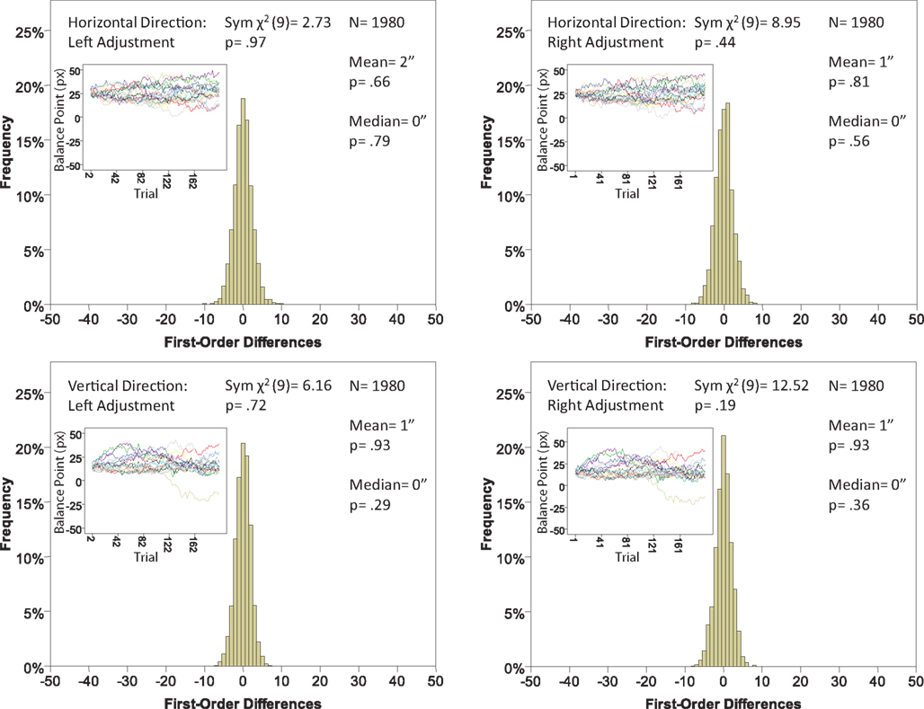
Figure 7. Histograms of the first-order differences (Δ’s) for the location experiment, participant LP. The insets show the time series of the matching adjustments from which the Δ’s were computed. Each panel contains the mean and the median of the corresponding Δ (in sec arc), with the p-values for the hypotheses that the population mean and median are 0, as well as the χ²(df = 9) and the p-value for the symmetry test described in the text.

FIGURE 8

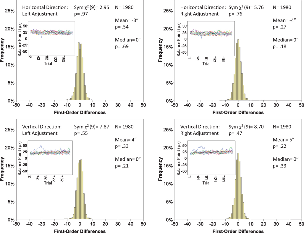
Figure 8. Histograms of the Δ’s for the location experiment, participant P1. The rest as in Figure 7.

FIGURE 9

Figure 9. Histograms of the Δ’s for the location experiment, participant P2. The rest as in Figure 7.

FIGURE 10

Figure 10. Histograms of the Δ’s for the location experiment, participant P3. The rest as in Figure 7.

FIGURE 11

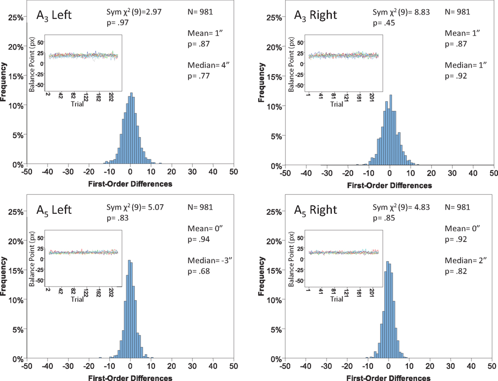
Figure 11. Histograms of the Δ’s for the shape experiment, participant LP. The rest as in Figure 7.

FIGURE 12

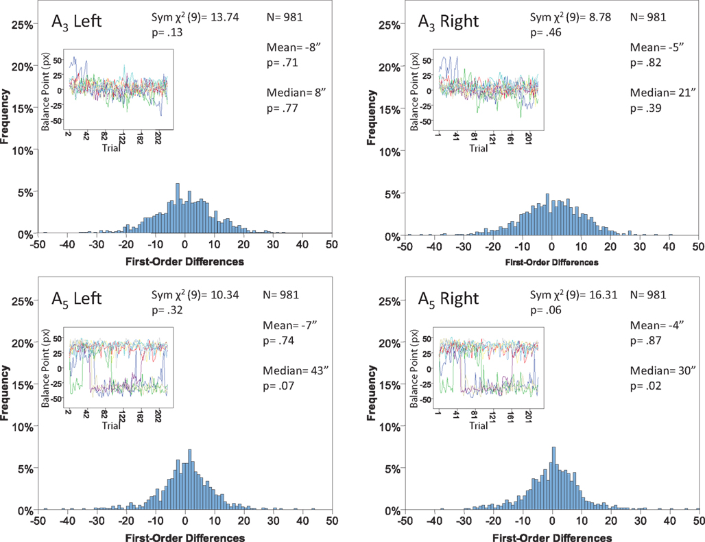
Figure 12. Histograms of the Δ’s for the shape experiment, participant P4. The rest as in Figure 7.

FIGURE 13

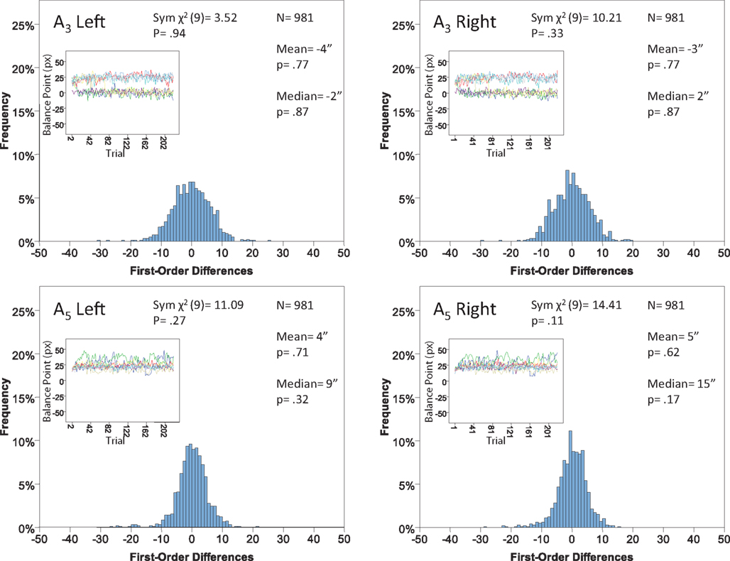
Figure 13. Histograms of the Δ’s for the shape experiment, participant P5. The rest as in Figure 7.

FIGURE 14

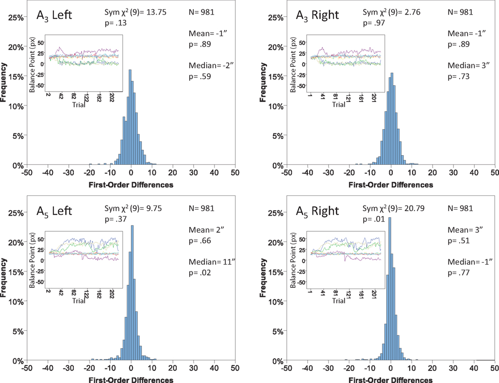
Figure 14. Histograms of the Δ’s for the shape experiment, participant P6. The rest as in Figure 7

FIGURE 15

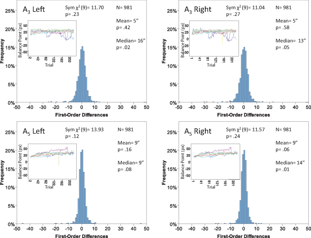
Figure 15. Histograms of the Δ’s for the shape experiment, participant P7. The rest as in Figure 7.

Each panel shows the results of three tests:

(H1₀) that the histogram of Δ’s is symmetric around 0 (against the generic alternative);

(H2₀) that the expected value of Δ is 0 (against the two-directional alternative), and

(H3₀) that the median Δ in the population is 0 (i.e., that Pr[Δ > 0] + Pr[Δ = 0]/2 = 1/2, against ≠1/2).

The symmetry in H1₀ means that Pr[Δ ∈ interval i] = Pr[Δ ∈ interval − i] for i = 1,…,9, where the intervals i are defined as

and

for the location experiment and the shape experiment, respectively. Note that the frequency of Δ’s in the intervals −9 and 9 was very small in the location experiment, which, combined with the fact that 8 pixels (≈492 sec arc) seems a good candidate for the notion of being “small,” was the reason for choosing this range for a “detailed view.” For uniformity, we used the same range for the shape experiment, although the frequency of Δ’s in the intervals −9 and 9 was not small for participants P5 and, especially, P4.

The test for the means was the standard t-test with the test statistic

The test for the medians was the χ²(df = 1) test with the test statistic

The symmetry test was the χ²(df = 9) test with the test statistic

6. Discussion

There are obvious individual differences in the patterns of the time series for balance points (the insets of the graphs). Our goal, however, is confined to their single feature: the lack or presence of a systematic trend, as revealed by the analysis of the first-order differences. In assessing the results, note that the choice of the significance level for a test (the alpha below which a p-value is considered rejecting the null hypothesis) is dubious when one deals with multiple tests: the computation of alpha depends on one’s subjective decision on how the different tests should be grouped. Setting the alpha for a given test for a given condition for a given participant in a given experiment at 0.05 means that the Type I error probability for 12 generally interdependent tests per participant per experiment (3 tests × 4 Δ’s) is anywhere between 0.05 and 0.6, making the overall Type I error probability across all tests for all conditions and all participants be anywhere between 0.19 and 0.97 for the location experiment, between 0.23 and 0.99 for the shape experiment, and between 0.37 and 1.0 if the two experiments are combined. The formula for these calculations is

where k is the number of tests per participant per experiment (in our case 12) and p is the number of independent applications of these k tests (four in the location experiment and five in the shape experiment), the tests for different participants × experiments being considered stochastically independent. To fix the lower boundary for the overall Type I error probability at 0.05 one needs to set the alpha for a given test × condition × participant × experiment at 0.013 for the locations experiment, at 0.010 for the shape experiment, and at 0.006 if the two experiments are combined. Rounding these figures to the conventional ones, we are justified to compare the p-values in our tests to 0.05 and 0.01. The results are summarized in Table 1.

TABLE 1

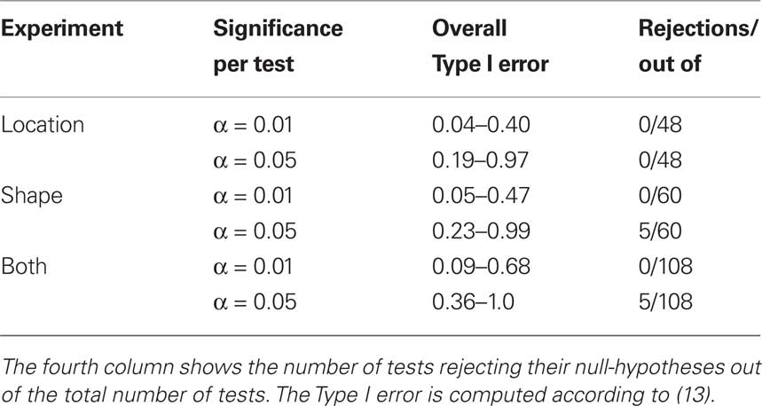
Table 1. An assessment of the results presented in Figures 7–10 (location experiment) and Figures 11–15 (shape experiment).

The conclusions one can derive from the location experiment are unequivocal. At α = 0.05 the null hypothesis is rejected in none of the 48 tests presented in the 16 panels of Figures 7–10 (although the probability of a rejection happening by chance, with all nulls true, is greater than 0.19). Equally important is that the values of the mean and the median are obviously very small (note that a single screen pixel measured 62 sec arc). The matching regularity hypothesis can be upheld for locations with very high confidence.

For the shape experiment none of the 60 tests presented in the 20 panels of Figures 11–15 rejects the null hypothesis at α = 0.01 (with the overall probability of Type I error exceeding 0.05). The hypothesis that the population means are 0 is not rejected at α = 0.05, and the mean Δ’s are very small. However, in one case out of 60 (Figure 14, right A₅) the distribution’s symmetry is rejected at α = 0.05, and the hypothesis that the population median is 0 is rejected at α = 0.05 in four out of 60 cases (right A₅ in Figure 12, left A₅ in Figure 14, left A₃ and right A₅ in Figure 15). Still, the logic of our tests leads us to conclude that for the shape experiment, too, there is little if any evidence against the null model of Sections 2.3 and 3.2. Note that there are no figure panels where we see a rejection occurring at α = 0.05 in more than one of the three tests. The occasional rejections can therefore be assumed to be Type I errors (whose probability in the shape experiment exceeds 0.23). Moreover, even if the rejected null hypotheses are indeed false, it is still possible (and probable, in view of the rest of the data) that these were the cases when the error terms were not sufficiently small to warrant dropping the o-terms in (12).

7. Conclusion

The symmetry of matching, ℳ𝒮 of Section 2.1, being a “natural” proposition firmly built in our colloquial language as well as in the language and practice of psychophysics, it seems to be a reasonable scientific strategy to dismiss this proposition only if the evidence against it is compelling. We have shown that in the matching-by-adjustment paradigm, with a reasonable definition of the PSE functions satisfying ℳℱ of Section 2.1, there is no empirical evidence against ℳ𝒮: y matches x if and only if x matches y.

Our paper does not, however, provide an algorithm for computing the precise matches for x and y from the distributions of the balance points Y_x and X_y, respectively. Rather, to the extent the use of the linear part of (12) is justifiable, our null model upholds the traditional textbook recommendation, usually confined to unidimensional stimuli (see, e.g., Gescheider, 1985, p.54): approximate the distribution of within-trial matches to a given stimulus by a normal distribution and take its mean as the (approximate) PSE for this stimulus. It is also common to advise (ibid) that if the distribution is not normal, a transformation may be applied first to make it normal. Our general model (Section 2.2) suggests a multidimensional version of the advice in question: transform the distribution of within-trial matches to a given stimulus into a normal distribution with uncorrelated components and then take its mean as the PSE for this stimulus. Glossing over statistical issues, this procedure provides a “direct access” to the variables a,b of (7), modulo linear transformations inconsequential for the analysis, making thereby the use of linear approximations unnecessary. Note that such transformations need not exist: thus, in the unidimensional case, no diffeomorphism would translate of which the first two are normal with distinct means and the third one is not normal, into three normal variates (Ghosh, 1969). An empirical demonstration that the transformation postulated in the general model does not exist would not necessarily falsify ℳ𝒮, but one would have then to seek other ways of operationalizing and testing it.

Appendix

We outline derivations of (10) and (11)–(12). For the kth trial pair,

where δa_k and δb_k are adjustment errors and |o| is o{1}|(δa_k,δb_k)|. Applying this recursively starting with k = 1, we get

where we use the notation [f]^p for f ○ f ○ …○ f (p times), and the |o|’s are o{1}|(δa₁,δb₁,…,δa_k−1,δb_k−1,δb_k)|. Recalling that x = T₁(a) and y = T₂(b), we get

with the |o|’s being o{1}|(δa₁,δb₁,…,δa_k,δb_k)|. It follows that

where the |o|’s are o{1}|(δa₁,δb₁,…,δa_k+1,δb_k+1)|. We get (10) after renaming the coefficients. Recalling the definition of H and G in (8), note that

In the null model g ≡ h⁻¹, and (14) becomes

This corresponds to (11). Note that the |o|’s here are o{1}|(δa₁, δb₁,…,δa_k+1, δb_k+1)|. Since the 3n-vector (δa_k, δa_k+1, δb_k+1) is identically distributed for all k, however, we can drop the index k altogether, denote the 3n-vector (δa, δa′, δb), and view the |o|’s as o{1}|(δa, δa′, δb)|. This yields (12).

Conflict of Interest Statement

The authors declare that the research was conducted in the absence of any commercial or financial relationships that could be construed as a potential conflict of interest.

Acknowledgments

This research has been supported by NSF grant SES 0620446 and AFOSR grant FA9550-09-1-0252 to Purdue University. The work has benefited from several discussions with Janne V. Kujala and R. Duncan Luce on the matching-by-adjustment paradigm and the issue of matching symmetry.

Footnotes

1. ^We use boldface letters, x,y,…, to denote stimulus values when we discuss stimuli of arbitrary nature (whether representable by numbers, functions, sets, names, etc.) and when stimulus values are known to be vectors of real numbers (as in the most of this paper). When stimulus values are single real numbers we may use lightface letters, x,y,….
2. ^This is an example of why it is always important to think of the x and y stimuli being compared as belonging to distinct “observation areas” (Dzhafarov, 2002b), such as left vs right, first vs second, left-and-red vs right-and-green vs left-and-green vs right-and-red, etc.
3. ^“Unidimensional” and “univariate” in this paper always mean “representable by real numbers.” Non-unidimensional stimuli can but need not be multidimensional (representable by vectors of real numbers): they may instead be representable by functions, sets, names, etc.
4. ^This is an example of the (re)labeling of stimuli mentioned in Section 2, resulting in all equivalent stimuli receiving one and the same label.
5. ^We have here another example of why it is always important to think of the x and y stimuli being compared as belonging to distinct observation areas. Transitivity or intransitivity of matching is usually discussed in terms of traditional triadic sequences (given x matched by y matched by z, is x matched by z?) but this does not make sense in the common case when there are just two observation areas (say, left and right) whereby z belongs to the same observation area with x (one cannot compare two “left” stimuli).
6. ^It is usually assumed that the values of x and y belong to the same set, but this assumption is not critical for our analysis. The latter would even apply to a case when x stimuli are, say, visual and y stimuli auditory.
7. ^The only property of these variables essential for this paper is their independence and symmetry around 0. The normality, however, is convenient due to the uniqueness properties mentioned at the end of this section.
8. ^In particular, the possibility of a special status of unidimensional stimuli was mentioned by Janne V. Kujala and R. Duncan Luce (personal communications to the first author, 2006).
9. ^This statement could have been strengthened: not only are not all the differences equal to 0, we know also that they are all positive or all negative. Our goal is, however, to formulate the H1_A as a simple negation of H1₀, so that one of them has to be true within the confines of the general model.

References

Beall, J. C. (2003). Liars and Heaps. Oxford: Oxford University Press.

Dzhafarov, E. N. (2002a). Multidimensional Fechnerian scaling: probability-distance hypothesis. J. Math. Psychol. 46, 352–374.

CrossRef Full Text

Dzhafarov, E. N. (2002b). Multidimensional Fechnerian scaling: pairwise comparisons, regular minimality, and nonconstant self-similarity. J. Math. Psychol. 46, 583–608.

CrossRef Full Text

Dzhafarov, E. N. (2003a). Thurstonian-type representations for “same–different” discriminations: deterministic decisions and independent images. J. Math. Psychol. 47, 208–228.

Dzhafarov, E. N. (2003b). Thurstonian-type representations for “same–different” discriminations: probabilistic decisions and interdependent images. J. Math. Psychol. 47, 229–243.

Dzhafarov, E. N. (2006a). Corrigendum to “Thurstonian-type representations for “same–different” discriminations: probabilistic decisions and interdependent images”: [Journal of Mathematical Psychology 47 (2003) 205–219]. J. Math. Psychol. 50, 511.

CrossRef Full Text

Dzhafarov, E. N. (2006b). On the law of regular minimality: reply to Ennis. J. Math. Psychol. 50, 74–93.

CrossRef Full Text

Dzhafarov, E. N., and Colonius, H. (2006). “Regular minimality: a fundamental law of discrimination,” in Measurement and Representation of Sensations, eds H. Colonius and E. N. Dzhafarov (Mahwah, NJ: Erlbaum), 1–46.

Dzhafarov, E. N., and Dzhafarov, D. D. (2010a). Sorites without vagueness I: classificatory sorites. Theoria 76, 4–24.

CrossRef Full Text

Dzhafarov, E. N., and Dzhafarov, D. D. (2010b). Sorites without vagueness II: comparative sorites. Theoria 76, 25–53.

CrossRef Full Text

Ennis, D. M. (2006). Sources and influence of perceptual variance: comment on Dzhafarov’s regular minimality principle. J. Math. Psychol. 50, 66–73.

CrossRef Full Text

Gescheider, G. A. (1985). Psychophysics: Method, Theory, and Application. Hillsdale, NJ: Erlbaum.

Ghosh, J. K. (1969). Only linear transformations preserve normality. Sankhya Ser A 31, 309–312.

Goodman, N. (1951/1997). The Structure of Appearance. Dordrecht: Reidel.

Keefe, R., and Smith, P. (1999). Vagueness: A Reader. Cambridge, MA: The MIT Press.

Khatri, C. G. (1987). Characterization of bijective and bimeasurable transformations of normal variates. Sankhya Ser A 49, 395–404.

Khatri, C. G., and Mukerjee, R. (1987). Characterization of bijective and bimeasurable transformations for bivariate normal variates. Sankhya Ser A 49, 405–411.

Kujala, J. V., and Dzhafarov, E. N. (2009). Regular minimality and Thurstonian-type modeling. J. Math. Psychol. 53, 486–501.

CrossRef Full Text

Luce, R. D. (1956). Semiorders and a theory of utility discrimination. Econometrica 24, 178–191.

CrossRef Full Text

Luce, R. D. (1977). Thurstone’s discriminal processes fifty year later. Psychometrika 42, 461–489.

CrossRef Full Text

Luce, R. D., and Edwards, W. (1958). The derivation of subjective scales from just noticeable differences. Psychol. Rev. 65, 222–237.

Pubmed Abstract | Pubmed Full Text | CrossRef Full Text

Luce, R. D., and Galanter, E. (1963). “Discrimination,” in Handbook of Mathematical Psychology, Vol. 1, eds R. D. Luce, R. R. Bush, and E. Galanter (New York: Wiley), 103–189.