Free-energy and illusions: the Cornsweet effect

In this paper, we review the nature of illusions using the free-energy formulation of Bayesian perception. We reiterate the notion that illusory percepts are, in fact, Bayes-optimal and represent the most likely explanation for ambiguous sensory input. This point is illustrated using perhaps the simplest of visual illusions; namely, the Cornsweet effect. By using plausible prior beliefs about the spatial gradients of illuminance and reflectance in visual scenes, we show that the Cornsweet effect emerges as a natural consequence of Bayes-optimal perception. Furthermore, we were able to simulate the appearance of secondary illusory percepts (Mach bands) as a function of stimulus contrast. The contrast-dependent emergence of the Cornsweet effect and subsequent appearance of Mach bands were simulated using a simple but plausible generative model. Because our generative model was inverted using a neurobiologically plausible scheme, we could use the inversion as a simulation of neuronal processing and implicit inference. Finally, we were able to verify the qualitative and quantitative predictions of this Bayes-optimal simulation psychophysically, using stimuli presented briefly to normal subjects at different contrast levels, in the context of a fixed alternative forced choice paradigm.

Introduction

Illusions are often regarded as “failures” of perception; however, Bayesian considerations often provide a principled explanation for apparent failures of inference in terms of prior beliefs. This paper is about the nature of illusions and their relationship to Bayes-optimal perception. The main point made by this work is that illusory percepts are optimal in the sense of explaining sensations in terms of their most likely cause. In brief, illusions occur when the experimenter generates stimuli in an implausible or unlikely way. From the subject’s perspective, these stimuli are ambiguous and could be explained by different underlying causes. This ambiguity is resolved in a Bayesian setting, by choosing the most likely explanation, given prior beliefs about the hidden causes of the percept. This key point has been made by many authors (e.g., Purves et al., 1999). Here, we develop it under biologically realistic simulations of Bayes-optimal perception and try to make some quantitative predictions about how subjects should make perceptual decisions. We then try to establish the scheme’s validity by showing that these predictions are largely verified by experimental data from normal subjects viewing the same stimuli.

The example we have chosen is the Cornsweet illusion, which has a long history, dating back to the days of Helmholtz (Mach, 1865; O’Brien, 1959; Craik, 1966; Cornsweet, 1970). This is particularly relevant given our formulation of the Bayesian brain is based upon the idea that the brain is a Helmholtz or inference machine (von Helmholtz, 1866; Barlow, 1974; Dayan et al., 1995; Friston et al., 2006). In other words, the brain is trying to infer the hidden causes and states of the world generating sensory information, using predictions based upon a generative model that includes prior beliefs. We hoped to show that the Cornsweet effect can be explained in a parsimonious way by some simple prior beliefs about the way that visual information is generated at different spatial and temporal scales.

The Cornsweet Effect and the Nature of Illusions

Figure 1 provides an illustration of the Cornsweet illusion. The illusion is the false percept that the peripheral regions of a stimulus have a different brightness, despite the fact they are physically isoluminant. This illusion is induced by a biphasic luminance “edge” in the centre of the field of view (shown in the right hand column of Figure 1). The four rows of Figure 1 show the Cornsweet effect increasing in magnitude as we increase the contrast of the stimulus. Interestingly, at high levels of contrast, secondary illusions – Mach bands (Mach, 1865; Lotto et al., 1999) – appear at the para-central points of inflection of the true luminance profile. It is this contrast-dependent emergence of the Cornsweet effect and subsequent Mach bands that we wanted to simulate, under the assumption that perception is Bayes-optimal.

FIGURE 1

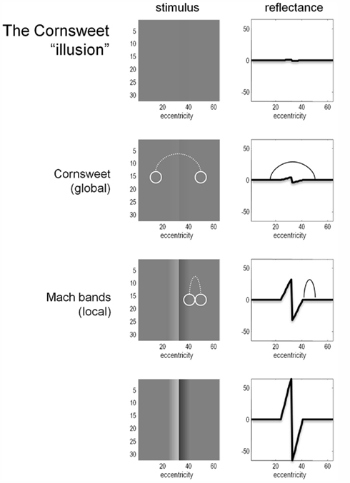
Figure 1. The Cornsweet illusion and Mach bands. The Cornsweet illusion is the false perception that the peripheral regions of a Cornsweet stimulus have different reflectance values. The magnitude of the effect increases as the contrast of the stimulus increases. At higher levels of contrast, the secondary illusion – Mach bands – appear. The Mach bands are situated at the point of inflection of the luminance gradient.

The Bayesian aspect of perception becomes crucial when we consider the nature of illusions. Bayesian theories of perception describe how sensory data (that have a particular likelihood) are combined with prior beliefs (a prior distribution) to create a percept (a posterior distribution). One can regard illusory percepts as those that are induced by ambiguous stimuli, which can be caused in different ways – in other words, the probability of the data given different causes or explanations is the same. When faced with these stimuli, the prior distribution can be used to create a unimodal posterior and an unambiguous percept. If the percept or inference about the hidden causes of sensory information (the posterior distribution) is different from the true causes used to generate stimuli, the inference is said to be illusory or false. However, with illusory stimuli the mapping of hidden causes to their sensory consequences is ill-posed (degenerate or many to one), such that a stimulus can have more than one cause. Thus, from the point of view of the observer, there can be no “false” inference unless the true causes are known. The perceptual inference can be optimal in a Bayesian sense, but is still illusory. However, not all possible causes of sensory input will be equally likely, so there will be an optimal inference in relation to prior beliefs about their causes. Prior beliefs can be learnt or innate: priors that are learnt depend upon experience while innate priors can be associated with architectural features of the visual brain, such as the complex arrangement of blobs, interblobs, and stripes in V1, that may reflect priors on the statistical structure of visual information selected by evolutionary pressure.

Prior beliefs are essential when resolving ambiguity or the ill-posed nature of perceptual inverse problems. Put simply, there will always be an optimal posterior estimate of what caused a sensation that rests upon prior beliefs. The example in Figure 2 illustrates this: The central panel shows an ambiguous stimulus (luminance profile) that is formally similar to the sort of stimulus that induces the Cornsweet illusion. However, this stimulus can be caused in an infinite number of ways. We have shown two plausible causes by assuming the stimulus is the product of (non-negative) illuminance and reflectance profiles. The lower two panels show the “true” causes generating stimuli for the Cornsweet illusion. Here, the stimulus has a reflectance profile that reproduces the Cornsweet stimulus and is illuminated with a uniform illuminant. An alternative explanation for exactly the same stimulus is provided in the upper two panels, in which two isoreflectant surfaces are viewed under a smooth gradient of ambient illumination. In this example, we have ensured that both the illuminant and reflectance are non-negative by applying an exponential transform before multiplying them to generate the stimulus.

FIGURE 2

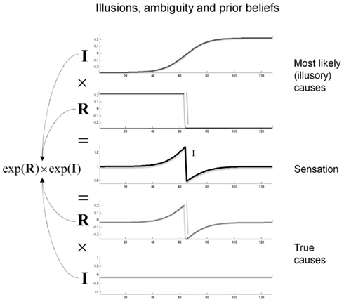
Figure 2. Contributions to luminance. Luminance values reaching the retina are modeled as a multiplication of illuminance from light sources and reflectance from the surfaces in the environment. The factorization of luminance is thus an ill-posed problem. One toy example of this degeneracy is shown here; the same stimulus can be produced by (at least) two possible combinations of illuminance and reflectance. Prior beliefs about the likelihood of these causes can be used to pick the most likely percept.

The key point made by Figure 2 is that there are many possible gradients of illuminance and reflectance that can produce the same pattern of sensory input (luminance). These different explanations for a particular stimulus can only be distinguished by priors on the spatial and temporal characteristics of the reflectance and illuminance. In this example, the ambiguity about what caused the stimulus can be resolved if we believe, a priori, that the visual world is composed of isoreflectant surfaces, as opposed to surfaces that (implausibly) get brighter or darker nearer their edges or occlusions (as in the lower panels). Under this prior assumption, an observer who infers the presence of spatially extensive isoreflectant surfaces, and explains the edge at the centre with an illuminance gradient, would be inferring its most likely cause. The Cornsweet “illusion” is thus only an illusion because the experimenter has chosen an unlikely combination of illuminance and reflectance profiles. In what follows, we will exploit priors on the spatial composition and generation of visual input to simulate the Cornsweet effect and the emergence of Mach bands.

The Bayesian approach to visual perception has been exploited in previous work (Yuille et al., 1991; Knill and Pouget, 2004). In addition, several other visual illusions have been explained using Bayesian principles, including motion illusions (Weiss et al., 2002), the sound-induced flash illusion (Shams et al., 2005), and the Chubb illusion (Lotto and Purves, 2001). Additionally, Purves et al. (1999) demonstrated the Bayesian nature of the Cornsweet illusion: when presented in a context implying an illuminance gradient and reflectance step, the Cornsweet illusion is elicited more easily.

In terms of the neuronal systems mediating the Cornsweet illusion; some authors have implicated subcortical structures: for example, Anderson et al. (2009) found that BOLD signal in the lateral geniculate nuclei (LGN) best correlated with perception of the Cornsweet illusion, although correlations were also seen in visual cortex. Furthermore, the illusion could be abolished if the stimulus was not presented binocularly, suggesting an origin before V1. Mach bands similarly have been attributed to retinal mechanisms (e.g., Ratliff, 1965); however, Lotto et al. (1999) have suggested a high-level contextual explanation for their appearance. Irrespective of the cortical or subcortical systems involved, we will assume, in this paper that the same Bayesian principles operate and, crucially, rest on a hierarchical generative model that necessarily implicates distributed neuronal processing at the subcortical and cortical levels.

Overview

This paper comprises three sections. The first describes a simple generative model of visual input that entails prior beliefs about how visual stimuli are generated and can be used to infer their causes. This model is used in the second section to simulate the perception of the Cornsweet illusion and contrast-dependent emergence of Mach bands. In the third section, we test the predictions of the simulations using a psychophysics study of normal subjects.

A Generative Model for the Cornsweet Effect

Our simulations are based upon the free-energy formulation of Bayes-optimal perception. Put briefly, this is based upon the notion that self-organizing agents minimize the average surprise (entropy) of sensory inputs through minimizing a free-energy bound on surprise. Here, surprise is just the improbability of sampling some sensory information, in relation to a (generative) model of how those sensations were produced. By adjusting the free parameters of the model, the sensory information can be explained or predicted and surprise minimized. Mathematically, surprise is the (negative) log evidence for a model of the world that comprises hidden variables (causes and states) that generate sensory information. We have described in many previous publications how this principle leads to active inference and Bayes-optimal perception (Friston et al., 2006; Friston, 2009; Feldman and Friston, 2010). Free-energy is a function of sensory samples and a probabilistic representation of what caused those samples. This representation can be cast in terms of the most likely or expected states of the world, under a generative model of how they conspire to produce sensory inputs. In brief, once we know the agent’s generative model, one can use the free-energy principle to predict its behavior and perception. In the present context, our focus will be on perception and the role of prior beliefs that are an inherent part of the generative model. In what follows, we describe the model and then use it to simulate perceptual inference and electrophysiological responses.

The Generative Model

The generative model we used is straightforward: sensory input is the product of reflectance and illuminance, where illuminance varies smoothly over space but can fluctuate with a high frequency over time. Conversely, the reflectance profile of the visual world is caused by isoreflectant fields or surfaces that fluctuate smoothly in time. Crucially, the spatial scales over which these fluctuations occur have a scale-free nature, of the sort found in natural images (Burton and Moorhead, 1987; Field, 1987; Tolhurst et al., 1992; Ruderman and Bialek, 1994; Ruderman, 1997). To ensure positivity of the illuminant and reflectance we apply an exponential transform to the two factors before multiplying them (as in Figure 2). Equivalently, we can imagine the underlying causes (reflectance and illuminance) as being composed additively in log-space. This model is shown schematically in Figure 3, in terms of hidden causes and states. Mathematically, this model can be expressed as:

FIGURE 3

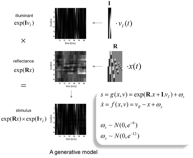
Figure 3. The generative model: the generative model employed in this paper models illuminance as a discrete cosine function and reflectance as a Harr wavelet function with peripheral high frequency wavelets removed. In addition, illumination is allowed to change quickly over time, whereas reflectance varies more slowly. This is achieved by making the coefficients on the reflectance basis functions hidden states, which accumulate hidden causes to generate changes in reflectance. Inversion of the model provides conditional estimates of the hidden causes and states responsible for sensory input as a function of time. See main text for an explanation of the variables in this figure.

Here, s(t) are sensory signals generated from hidden states x(t) and causes, v(t) plus some random fluctuations ω(t). The difference between hidden causes and states is that states evolve dynamically, in response to perturbations by hidden causes – these dynamics are described by the equation of motion in the second equality above. Hidden causes v(t) = (v_I, v_R) have been divided into those causing changes in luminance and those causing changes in hidden states that produce changes in reflectance. These hidden variables control the amplitude of spatial basis functions (R, I) encoding formal beliefs about the spatial scales of illuminance and reflectance. For the illuminant (I) we use a low-order discrete cosine transform, while for the reflectant (R) we use a low-order discrete wavelet transform.

The particular wavelet transform used here is a Haar wavelet set that has been thinned by removing high-order wavelets (with high spatial frequency) from the periphery of the visual field: This respects, roughly, the increasing size of classical receptive fields with retinotopic eccentricity. For simplicity (and ease of reporting the results), we restrict the simulations to a one-dimensional visual field. Because Haar wavelets afford local linear approximations to continuous reflectance profiles, the resulting reflectance has to be a mixture of isoreflectant surfaces at different spatial scales. To impose the scale-free aspect, we decrease the variance or, equivalently, increase the precision of the reflectance wavelet coefficients or hidden states in proportion to the order or spatial scale of their wavelet. This is implemented by placing a prior on the wavelet coefficients with the form p(x_k) = N(0, e^−3k), where k is the order of the wavelet. Neuronally, these basis functions could stand in for a filling-in process such as that described by Grossberg and Hong (2006). Conversely, the illuminant is modeled as a mixture of smoothly varying cosine functions with a low spatial frequency. This is easily motivated by the fact that most sources of illumination are point sources, which results in smooth illuminance profiles. These were modeled here with the first three components of a discrete cosine transform (see Figure 4 for a graphical representation of the basis functions and how they are used to generate a stimulus).

FIGURE 4

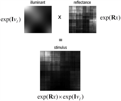
Figure 4. Two-dimension example. The top panels show 2-D examples of luminance (left) and reflectance (right), created form the generative model. The resulting stimulus is the product of the two (bottom panel).

By construction, this generative model of visual signals separates the spatial scales or frequencies of the illuminance and reflectance such that all the high frequency components are in the reflectance profile, while the low frequency components are in illuminance profile. Temporal persistence of reflectance is assured because the reflectance coefficients x(t) ∈ ℜ^{16 × 1} are hidden states that accumulate hidden causes v_R(t) ∈ ℜ^{16 × 1}. This persistence reflects the prior belief that surfaces move in a continuous fashion. For simplicity, we mapped the hidden causes controlling illuminance v_I(t) ∈ ℜ^{3 × 1} directly to the stimulus (although this is not an important feature of our model). This can be thought of as accommodating rapid changes in illuminance of the sort that might be produced by a flickering candle.

Equation 1 defines our generative model in terms of the joint probability over sensory information and the hidden variables producing fluctuations in reflectance and illuminance. The fluctuations in the hidden causes are assumed to be Gaussian with a precision (inverse variance) of one, while the fluctuations in the motion of the hidden states are assumed to have a log-precision of 12. Finally, we assume sensory fluctuations or noise with a log-precision of six. In the next section, we will manipulate the log-precision of the sensory noise as a proxy for changing the contrast of the stimulus.

Figure 4 shows a snapshot of the sort of visual signals this generative model produces. Here, we have used the outer product of the discrete transforms above to generate a two-dimensional stimulus. We are not pretending that this is a veridical model of the real visual world. However, it is sufficient to explain the Cornsweet illusion and related effects by incorporating simple and plausible priors on the spatial scales over which illuminance and reflectance change. In the next section, we use this generative model to simulate perceptual and physiological responses to a stimulus, under the free-energy principle. This reduces to a Bayesian deconvolution of sensory input that tries to discover the most likely hidden causes and states generating that input.

Perception and Predictive Coding

This perceptual deconvolution can be regarded as the inversion of a generative model that maps from hidden causes (variables in the world) to sensory consequences. The inverse mapping corresponds to inferring those variables by mapping back from the sensory consequences to the hidden causes and states. This can be implemented in a biologically plausible fashion using a generalized gradient descent on variational free-energy which is a function of (generalized) sensory states and the expected values μ(t) = (μ_x, μ_v) of hidden variables (see Friston, 2008 for details). In brief, this gradient descent corresponds to a Bayesian filtering, in which expected states of the world are continuously optimized using a prediction term and an update term:

Under the simplifying assumption that probabilities are represented as Gaussian densities, this can be regarded as a generalized form of Kalman filtering, where the second (update or gradient) term can be expressed as a mixture of prediction errors (see the equations in Figure 5). This means that the generalized filtering inEq. 2to corresponds to a generalized form of predictive coding. Predictive coding has become a popular metaphor for understanding perceptual inference in the visual system. For example, Rao and Ballard (1999) used predictive coding to provide a compelling explanation for extraclassical receptive field effects in striate cortex.

FIGURE 5

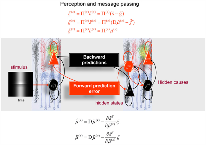
Figure 5. Hierarchical message-passing in the brain. The schematic details a neuronal architecture that optimizes the conditional expectations of hidden variables in hierarchical models of sensory input of the sort illustrated in Figure 3. It shows the putative cells of origin of forward driving connections that convey prediction error from a lower area to a higher area (red arrows) and non-linear backward connections (black arrows) that construct predictions (Mumford, 1992; Friston, 2008). These predictions try to explain away (inhibit) prediction error in lower levels. In this scheme, the sources of forward and backward connections are superficial and deep pyramidal cells (triangles) respectively, where state-units are black and error-units are red. The equations represent a generalized gradient descent on free-energy (see main text) using the generative model of the previous figure. If we assume that synaptic activity encodes the conditional expectation of states, then recognition can be formulated as a gradient descent on free-energy. Under Gaussian assumptions, these recognition dynamics can be expressed compactly in terms of precision weighted prediction errors: ξ⁽ⁱ⁾:i = s, x, v on the sensory input, motion of hidden states, and the hidden causes. The ensuing equations suggest two neuronal populations that exchange messages; with state-units encoding conditional predictions and error-units encoding prediction error. Under hierarchical models, error-units receive messages from the state-units in the same level and the level above; whereas state-units are driven by error-units in the same level and the level below. These provide bottom-up messages that drive conditional expectations μ⁽ⁱ⁾:i = x, v toward better predictions to explain away prediction error. These top-down predictions correspond to that are specified by the generative model. This scheme suggests the only connections that link levels are forward connections conveying prediction error to state-units and reciprocal backward connections that mediate predictions. Note that the prediction errors that are passed forward are weighted by their precisions: Π⁽ⁱ⁾:i = s, x, v. Technically, this corresponds to generalized predictive coding because it is a function of generalized variables, which are denoted by a (∼), such that every variable is represented in generalized coordinates of motion: for example: See Friston (2008) for further details.

Put simply, in these simulations we assume that neural activity corresponds to the brain’s representation of the most likely values of the hidden causes and states (hidden variables) and that these are continuously updated to minimize free-energy. The ensuing scheme has been discussed in terms of recurrent message-passing among different cell populations in hierarchical sensory cortex: see Figure 5 and Mumford (1992). This scheme rests upon the use of bottom-up prediction errors to optimize conditional estimates of hidden variables. These estimates are then used to produce top-down predictions that are compared with sensory input to form a bottom-up prediction error. In this context, the sum of squared prediction error can be regarded as free-energy. The recursive message-passing used in these schemes tries to minimize prediction error, such that the predictions approximate the true conditional or posterior estimates of the underlying hidden causes. It is this message-passing that we will stimulate in the next section and associate with neuronal responses, while using what they represent to predict how real subjects would respond behaviorally, in terms of their perceptual decisions or inference.

To simulate these responses we simply integrate or solveEq. 2, using the functions g(x, v) and f(x, v) specified by a generative model inEq. 1. These functions map hidden variables to sensory input and encode prior beliefs about the dynamics of hidden states. In short, by plugging the equations of our generative model in Figure 3 into the predictive coding scheme of Figure 5, we can simulate Bayes-optimal inference about the causes of sensations. Crucially, we can then reconstitute the posterior or conditional beliefs about these causes and associate these with percepts. In particular, we can take any mixture of the hidden variables and assess the posterior belief about that mixture. We will use this to quantify the Cornsweet and Mach band percepts, in terms of reflectance differences among different parts of the visual field. Note that the predictive coding scheme in Figure 5 weights the prediction errors by precision matrices. For example, the precision of sensory signals is Π^(s) = I·exp(γ). These precisions are functions of log-precisions γ that encode the expected amplitude of random fluctuations.

Simulated Responses

The simulated responses in Figure 6 were obtained by presenting the Cornsweet stimulus under uniform illumination. Here, the stimulus was presented transiently by modulating the illumination with a Gaussian envelope over time (see image inset). The resulting predictions are shown in Figure 6A as solid lines, while the red dotted lines correspond to the prediction error. These predictions are based upon the inferred hidden states and causes shown on the right and lower left respectively. The lines correspond to the posterior expectations and the gray regions correspond to 90% Bayesian confidence intervals. In terms of the underlying causes, the blue curve in Figure 6B is an estimate of the (log) amplitude of uniform illumination. This should have a roughly quadratic form (given the Gaussian envelope), peaking at around bin 30, which indeed it does. The remaining causes that deviate from zero (Figure 6C) are the perturbations to the hidden states explaining or predicting changes in reflectance. These drive increases or decreases in the conditional expectations of the hidden states shown on the right. The green line is the coefficient of the second-order basis function splitting the visual field into an area of brightness on the left and darkness on the right. It can be seen that at the point of maximum illumination, there is an extremely high degree of confidence that this hidden state is bigger than zero. This is the Cornsweet percept.

FIGURE 6

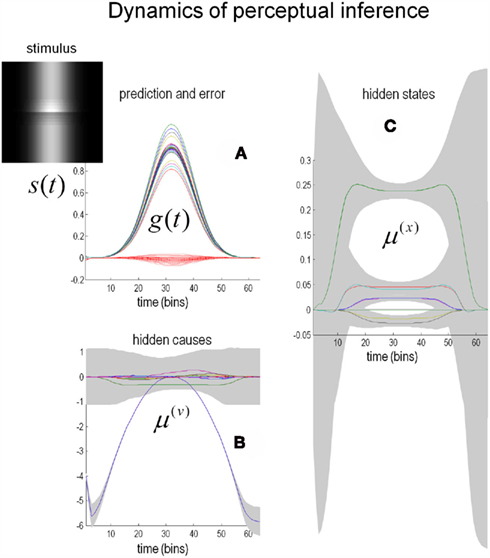
Figure 6. Predictions of the model. (C) Shows the estimates of the hidden states (coefficients of the reflectance basis functions) over time. The hidden state controlling the amplitude of the lowest-frequency basis function, which corresponds to the Cornsweet percept, contributes substantially to the overall perception of the stimulus (green line). The estimates for the hidden causes are shown in (B). The gray areas are 90% confidence intervals. (A) Shows predictions (solid lines) of sensory input based on the estimated hidden causes and states and the resulting prediction error (dotted red lines). The insert on the upper left shows the time-dependent luminance profile used in this simulation. Please see main text for further details.

The corresponding percepts in sensory space are shown in Figure 7 as a function of peristimulus time. The upper panels show the implicit reflectance and illuminance profiles encoded by the conditional expectations of hidden variables respectively. After an exponential transform (and multiplication) these produce the sensory predictions shown on the lower left. By taking a weighted mixture of the perceived reflectance in different regions of the visual field (shown by the white circles) one can estimate the conditional certainty about both the Cornsweet effect (differences in perceived reflectance on different sides) and the appearance of Mach bands (differences in perceived reflectance on the same side). The weights used to evaluate these mixtures are denoted as W_corn and W_mac for the Cornsweet and Mach band effects respectively. The conditional expectation of these mixtures or effects μ_mac = W_mac·μ^(x) and their confidence intervals are shown on the lower right. At this level of visual contrast or precision (a log-precision of six), the Cornsweet effect is clearly evident with a high degree of certainty, while the confidence interval for the Mach band effect always contains zero. In other words, at this contrast (sensory precision) there is a Cornsweet effect but no Mach band effect. In the next section, we repeat the simulation above and record the conditional expectations (and confidences) about illusory effects at the point of maximum illumination for different levels of contrast.

FIGURE 7

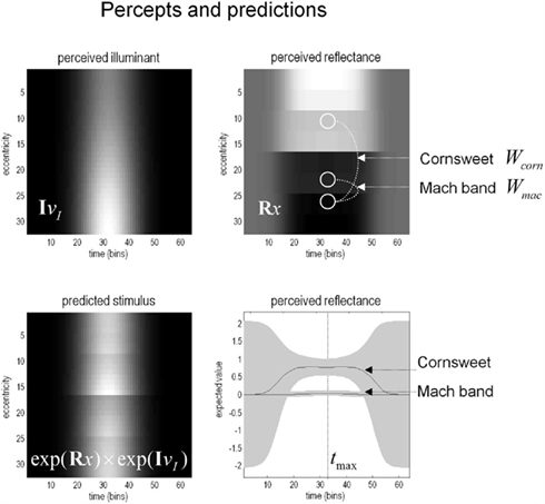
Figure 7. The model’s “perceptions.” The upper panels show the predicted illuminance (left) and reflectance profiles (right), reconstructed from the coefficients of the basis functions estimated from the model inversion shown in the previous figure. An inferred reflectance profile demonstrating the Cornsweet illusion is apparent, but at this level of contrast, Mach bands have not yet appeared. Please see main text further details.

Contrast or Precision-Dependent Illusory Percepts

Using the generative model and inversion scheme described above, we repeated the simulations over different levels of sensory precision. This can be regarded as a manipulation of contrast in the following sense: If we assume that the brain uses divisive normalization (Weber, 1846; Fechner, 1860; Craik, 1938; Geisler and Albrecht, 1992; Carandini and Heeger, 1994), the key change in sensory information, following an increase in contrast, is an increase in signal to noise; in other words, its precision increases (see the appendix of Feldman and Friston, 2010 for details). We use therefore a manipulation of the log-precision of sensory noise to emulate changes in visual contrast. It should be noted that we did not actually add sensory noise to the stimuli. The key quantity here is the level of precision assumed by the agent which, in these simulations, we changed explicitly. In more realistic simulations, the log-precision would be itself optimized with respect to free-energy (see Feldman and Friston, 2010 for an example of this in the modeling of attention).

Figure 8 shows the results of perceptual inference under the Bayesian scheme described above. The only thing that we changed was the log-precision of the sensory input, from minus two (low) through to intermediate levels and ending with a very high log-precision of 16. The two graphs show the conditional expectation and 90% confidence intervals for the Cornsweet effect (upper panel) and Mach bands (lower panel) respectively, at the point of maximum illumination. It can be seen in both instances that under low levels of contrast (sensory precision) both effects are very small and inferred with a large degree of uncertainty. However, as contrast increases, conditional uncertainty reduces and, at a critical level, produces a confident inference that the effect is greater than zero (or some small threshold). Crucially, the point at which this happens for the Cornsweet effect is at a lower level of contrast than for the Mach bands. In other words, the Cornsweet illusion occurs first and then the Mach bands appear as contrast continues to rise. The explanation for this is straightforward; the Mach band illusion rests upon higher spatial frequencies in the generative model, which have a higher prior precision (encoding prior beliefs about the statistical – scale-free – structure of natural visual scenes). This means that there needs to be precise sensory evidence to change them from their prior expectation of zero. In short, at high levels of contrast or sensory precision, more and more fine detail in the posterior percept is recruited to provide the optimum explanation for the stimulus. Interestingly, as the contrast or sensory precision reaches very high levels, the veridical reflectance and illuminant profiles are inferred and, quantitatively, both the Cornsweet and mach band effects disappear. The three images show exemplar percepts, at low, intermediate and high levels of contrast respectively. The key difference in the spatial banding that underlies the Cornsweet and Mach band effects is evident in the difference between the intermediate and high levels of contrast.

FIGURE 8

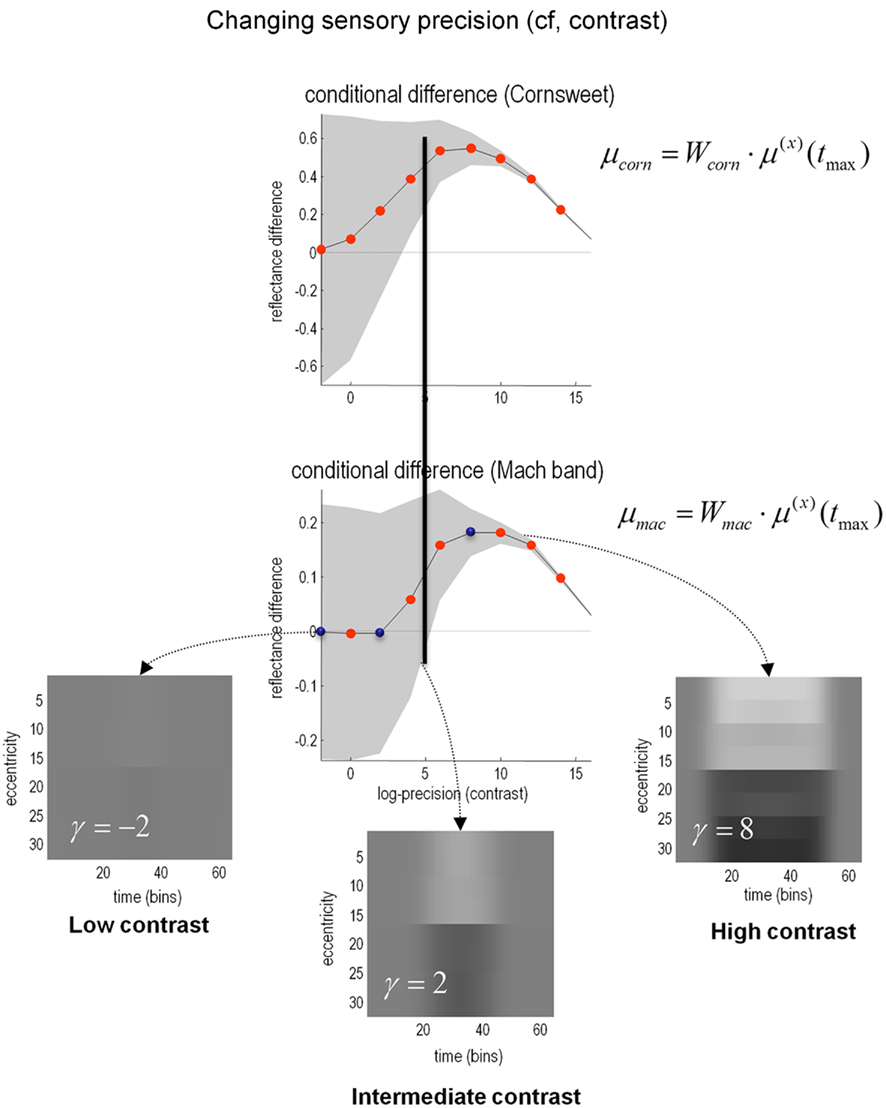
Figure 8. The effect of contrast. In the results presented here the precision of the sensory data was used as a proxy for stimulus contrast. As precision increases, the strength of both the Cornsweet and Mach effects increases until, at very high levels of precision (contrast) the true luminance profile is perceived and the illusory percepts fade. Crucially, the Mach bands appear at higher levels of contrast than the Cornsweet illusion. The inserts in the lower panels show the inferred reflectance is at different levels of contrast (indicated by the blue dots in the lower graph). The prediction errors associated with the processing of stimuli at these three levels are shown in the next figure. Please see main text for further details.

The key prediction of these simulations is that we would expect subjects to categorize their percepts, following a brief exposure to a Cornsweet stimulus, differently at different levels of contrast. At low levels of contrast, we would expect them to categorize the stimulus as uniformly flat. At intermediate levels of contrast, we would expect them to categorize the stimulus as a Cornsweet percept, with isoluminant and uniform differences in the right and left hand parts of the visual field; while at higher levels of contrast one would expect the Mach bands to dominate and the stimuli would be categorized as possessing para-central bands. In principle, at very high levels of contrast, the subject should perceive the veridical stimulus. However, whether this level of contrast can be attained empirically is an open question. In the next section, we test these hypotheses psychophysically. We conclude this section by looking not at behavioral responses but at the neuronal responses implicit in the simulations.

Simulating Neuronal Responses

Figure 9 shows the prediction errors at low, intermediate and high levels of contrast. These are shown at the sensory level (upper row) and at the higher levels of the hidden causes and states (lower row). The key thing to note here is that as contrast increases and the spatial detail of the posterior predictions increases, the sensory prediction error falls. This is at the expense of inducing prediction errors at the higher level, which increase in proportion to the precision of sensory information. These higher prediction errors are simply the difference between the posterior and prior expectations and reflect an increasing departure from a prior expectation of zero as contrast (the log-precision of sensory noise) increases. Although these results are interesting in themselves, they can also be regarded as a simulation of event related potentials. The reason that we can associate prediction error with observed electromagnetic brain responses is that it is usually assumed that prediction errors are encoded by the activity of superficial pyramidal cells (see Figure 5). It is these cells that are thought to contribute primarily to local field potentials and non-invasive EEG signals.

FIGURE 9

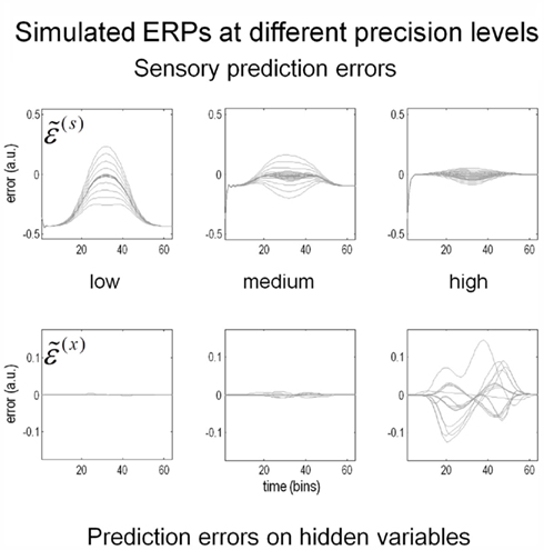
Figure 9. Contrast and prediction error. As stimulus contrast increases, prediction error is redistributed from sensory input to hidden variables. At high levels of precision, sensory information induces prediction errors at higher levels, which in turn explain away prediction error at the sensory level. The higher level prediction errors at high precision reflect increasing confidence that the reflectance is different from the prior expectation of zero. Please see main text for further details.

In the high-contrast condition, the prediction errors at the lower level are suppressed by the prediction of the presence of a Cornsweet stimulus. This sort of phenomenon has been demonstrated using fMRI (Alink et al., 2010; den Ouden et al., 2010); predictable stimuli cause less activation in stimulus-specific areas than unpredictable stimuli. However, the process simulated here is likely to produce more complicated neurophysiological correlates because of the confounding effect of precision; increased predictability (through increasing conditional confidence about the stimulus) will also increase estimates of precision. Since we believe that the prediction errors reported by superficial pyramidal cells are precision weighted, decreasing prediction error in lower sensory areas may be masked by the increasing precision of those errors. We will return to this and related issues in a subsequent paper looking at the neurophysiological correlates of contrast-dependent illusory effects. Here, we focus on psychophysical correlates:

A Psychophysical Test of Theoretical Predictions

In this section, we report a psychophysics study of normal subjects exposed to the same stimuli used in the simulations above. We depart from the normal procedures for assessing illusions (which usually involve matching intensity differences) by using a forced choice paradigm. This is because we wanted to present stimuli briefly, for several reasons: First, brief presentation avoids the confounding effects of saccadic eye movements. Second, it allows us to prototype the paradigm for future use in electrophysiological (event related potential) studies, which require transient stimuli for trial averaging. Finally, a forced choice paradigm places constraints on the subject’s choices that map directly to the model predictions. In what follows, we describe the paradigm and interpret our results quantitatively, in relation to the predictions of the simulations above.

Subjects and Experimental Paradigm

We studied normal young subjects in accord with guidelines established by the local ethical committee and after obtaining informed consent. Eight participants (4 female) completed the Mach band paradigm; 19 (12 female) completed the Cornsweet paradigm.

Experiment 1 (Cornsweet Paradigm)

The Cornsweet illusion was assessed using a two-interval forced choice procedure. Subjects were presented with a (set contrast) Cornsweet stimulus and real luminance step for 200 ms (a Gaussian temporal envelope was not used), separated by an interval of 200 ms. One stimulus appeared to the left of fixation and one to the right; this was randomized across trials, as was the order of the stimuli. Subjects were asked to report the side on which the stimulus with the greatest contrast had appeared (Figure 10).

FIGURE 10

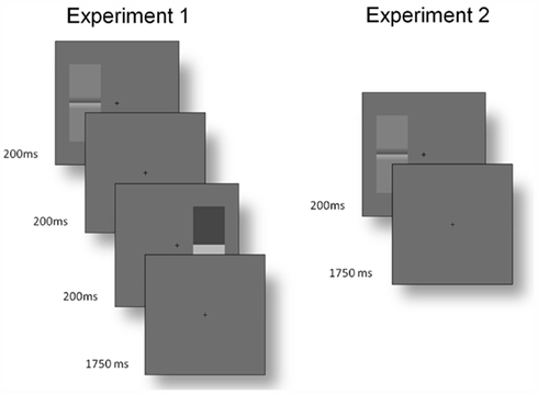
Figure 10. Time courses of trials. Experiment 1: before the start of each trial, participants fixated a central cross. One Cornsweet and one real luminance step stimulus appeared for 200 ms each, with a 200 ms interval between them. The order of the stimuli, their orientation and the side on which each appeared were randomized (although they were constrained to appear on opposite sides within each trial). Participants then had 1750 ms to report the side on which the stimulus with the greatest contrast had appeared (using the arrow keys of the keyboard). Experiment 2: each trial stared with fixation. A Cornsweet stimulus then appeared for 200 ms with a random orientation to the left or right of fixation. Participants had 1750 ms to report, with the “Y” and “N” keys, if they perceived Mach bands.

Six blocks were completed, using Cornsweet stimuli with Weber contrasts of 0.0073–0.734. A Quest procedure (Watson and Pelli, 1983) was used to select each step stimulus for comparison. The mean of the psychometric function was taken as the point of subjective equality between the Cornsweet stimulus and a real luminance. There were 200 presentations per block.

Experiment 2 (Mach Band Paradigm)

The same method could not be used to identify the strength of the Mach bands percept, as there is no non-illusory stimulus that can be used for matching. Consequently, we used a two-alternative forced choice paradigm: A single Cornsweet stimulus was displayed for 200 ms to the left or right of fixation and participants were asked to report if the stimulus contained Mach bands or not. Each participant completed six runs of 200 presentations at 10 Weber contrast levels from 0.0204 to 0.2038. The probability of reporting a Mach band was assessed as the relative frequency of reporting its presence over trials, within subject (Figure 10).

In both experiments, stimuli were displayed on an LCD monitor under ambient room lighting. Subjects were seated 60 cm away from the monitor, such that stimuli subtended an angle of 14.21° vertically and 6.10° horizontally, at 2.96°–7.06° eccentricity. The luminance ramp of the Cornsweet stimulus profile occupied 2.42°. Only the lowest levels of contrast the monitor was able to produce were employed; thus, luminance values were linearized post hoc.

Results and Discussion

The results of the psychophysics experiments are shown in Figure 11, as a function of empirical (Weber) contrast levels. These results are expressed as the mean over all subjects and associated SE. The reported Cornsweet effect (as indexed by the point of subjective equality) peaked, on average over subjects, at a contrast of about 0.0025. At higher levels of contrast, as in the simulations, the effect fell quantitatively, plateauing at the highest contrast used in Experiment 1. Conversely, the probability of reporting a Mach band increased monotonically as a function of the empirical contrast, reaching about 75% at a Weber contrast of about 0.15.

FIGURE 11

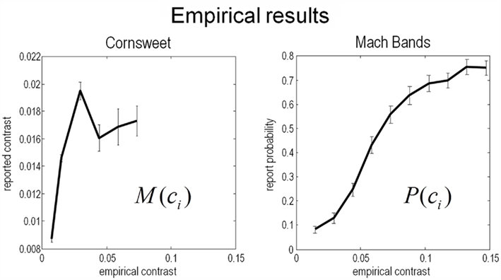
Figure 11. experimental results. This figure shows the results of the empirical psychophysical study for the Cornsweet illusion (left panel) and the Mach band illusion (Right panel). Both report the average effect over subjects and the SE (bars). The Cornsweet illusion is measured in terms of the subjective contrast level (quantified in terms of subjective equivalence using psychometric functions). The Mach band illusion is quantified in terms of probability that the illusion is reported to be present. Both results are shown as functions of empirical (Weber) stimulus contrast levels. We have used the same range for both graphs so that the dependency on contrast levels can be compared. The key thing to note here is that the Cornsweet illusion peaks before the Mach band illusion (vertical line).

Qualitatively, these empirical results compare well with the theoretical predictions shown in Figure 9: that is, the subjective or inferred Cornsweet effect emerged before the Mach bands, as contrast increases. We also see the characteristic “inverted U” dependency of the Cornsweet effect on contrast levels. The empirical profile is somewhat compromised by the small range of contrasts employed, however, this range was sufficient to disclose an unambiguous peak. Clearly, it would be nice to relate these empirical results quantitatively to the simulations shown in Figure 9. This presents an interesting challenge because the psychophysical data consist of reported levels of an effect and the probability of an effect for the Cornsweet and Mach Band illusions respectively. However, because our simulations provide a conditional or posterior probability over the effects reported, we can simulate both sorts of reports and see how well they explain the psychophysical data. This quantitative analysis is now considered in more detail.

A Formal Behavioral Analysis

The simulations provide conditional expectations (and precisions) of both the Cornsweet and Mach band effects over a number of simulated (Weber) contrast levels, as modeled with the precision of sensory noise. This means that one can compute a psychometric function of contrast c that returns the behavioral predictions of both illusions respectively; namely, the level of the illusion and the probability of inferring a Mach band. To predict the reported level of the Cornsweet illusion we can simply use the conditional expectation μ_corn(c) scaled by some (unknown) coefficient β₁. To predict the probability of reporting the presence of Mach bands, one can integrate the conditional probability distribution over the Mach band effect above some (unknown) threshold β₂. However, to do this, we need to know the relationship between the simulated and empirical contrasts:

As noted above, we used the log-precision of sensory noise γ to model log-contrast in accord with Weber’s law. This means we can assume a linear relationship between the empirical log-contrast and simulated log-precision. This induces two further unknown coefficients – the slope and intercept (β₃ and β₄) that parameterise the relationship between the simulated and empirical contrasts. Finally, we need to relate the conditional probability of a suprathreshold Mach band effect to the probability of reporting its presence. Here, we assumed a simple, monotonic sigmoid relationship, under the constraint that when the conditional probability was 50:50, the report probability was also 50:50. The precise form of this mapping is provided in Figure 11 (left panel) and has a single (unknown) slope coefficient β₅. These relationships provide a mapping between the results of the simulations and the observed responses averaged over subjects (under the assumptions of additive prediction errors). This is known as a response model and is detailed schematically in Figure 11. The predictions are based on the simulated responses in Figure 9, assuming a smooth psychometric function of contrast that was modeled as a linear mixture of cosine functions: X_k(γ) = cos(πγk) for k = 1, …, 6). The coefficients of this discrete cosine set were estimated with ordinary least squares, using the responses of the model (μ_corn(γ), μ_mac(γ)) over different precision levels, at the time of maximum luminance.

Given the form of the relationships between the simulated and empirical contrasts and between the report probability and conditional probabilities for Mach bands, one can use the psychophysical data to estimate the unknown coefficients of these relationships: β_i for = 1,…, 5. The results of this computationally informed response modeling are shown in the right panel of Figure 12. The upper panels show the same data as in Figure 10 placed over the theoretical psychometric functions based on the simulations of the previous section. These predictions are based on the mapping from simulated to empirical contrast levels (lower left) and the relationship between the probability of reporting a Mach band and the conditional confidence that it is present (lower right).

FIGURE 12

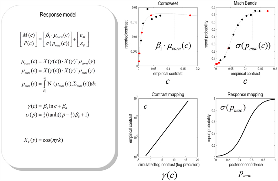
Figure 12. Predicted and experimental results. Theoretical predictions of the empirical results reported in the previous figure: These predictions are based upon a response model that maps from the conditional expectations and precisions in the simulations to the behavioural responses of subjects. This mapping rests on some unknown parameters or coefficients β_i:i = 1, …, 5 that control the relationship between the simulated γ(c) and empirical contrast levels c used for stimuli and the relationship between the probabilities of reporting a Mach band σ(p_mac(c)) and the conditional probability that it exceeds some threshold p_mac(c) at contrast level c. These relationships form the basis of a response model, whose equations are provided in the left panel (for simplicity, we have omitted the expressions for conditional variance of the Mach band contrast). Given empirical responses for the mean Cornsweet effect M(c) and probability of reporting a Mach band P(c), the coefficients β_i can be estimated under the assumption of additive prediction errors ε. The predicted responses following this estimation are shown in the graphs on the right hand side. The upper panels show the empirical data superimposed upon conditional predictions from the model. The gray lines are the predicted psychometric functions, μ_corn(c) and σ(p_mac(c)). The red dots correspond to the predictions at levels of contrast used in the simulations (as shown in Figure 9), while the black dots correspond to the empirical responses: M(c) and P(c). The lower left panel show the relationship between the empirical and simulated contrast levels (as a semi-log plot of the empirical contrast against the log-precision of sensory noise). The lower right panel shows the relationship between the probability of reporting a Mach band is present and the underlying conditional probability that it is above threshold.

By construction, the relationship between the simulated and empirical contrasts is linear when plotted on a log-log scale. The slope of this plot suggests that the higher contrasts used in the simulations are, practically, not realizable in an empirical setting. This is because as the simulated contrast increases the corresponding empirical contrast increases much more quickly. The implication of this is that the contrasts employed in the psychophysics study correspond to the first few levels of the simulated contrasts. This means that it may be difficult to demonstrate the theoretically predicted attenuation of the Cornsweet illusion at very high levels of contrast.

The relationship between the report and conditional probabilities suggests that subjects have a tendency to “all or nothing” reporting; in the sense that a conditional confidence that the probability of reporting a Mach band is slightly greater than the conditional confidence it is above threshold. Conversely, subjects appear to report the absence of Mach bands with a probability that is slightly greater than the conditional probability it is below threshold. The resulting psychometric predictions (in the upper panels) show a remarkable agreement between the predicted and observed probabilities of reporting a Mach band. The correspondence between the predicted and empirical results for the Cornsweet illusion are less convincing but show that both asymptote to a peak level much more quickly than the probability of reporting a Mach band.

In summary, this analysis suggests that there is a reasonable quantitative agreement between the theoretical predictions and empirical results. Furthermore, in practical terms, it appears that the normal range of Weber contrasts that can be usefully employed corresponds to a relatively low level of sensory precision in the simulations. This means that it may be difficult to demonstrate the “inverted U” behavior for the Cornsweet illusion seen in Figure 9. This is because it may be difficult to present stimuli at the ultra high levels of contrast required. Note that the empirical probability of reporting a Mach band does not decrease as a function of contrast level. This is to be anticipated from the theoretical predictions: increasing the contrast level increases the conditional precision about the inferred level of the Mach band effect, which means that the probability that is above threshold can still increase even if the conditional expectation decreases (as in Figure 9).

Conclusion

This paper has reviewed the nature of illusions, in the context of Bayes-optimal perception. We reiterate the notion that illusory percepts are optimal in that they may represent the most likely explanation for ambiguous sensory input. We have illustrated this using the Cornsweet illusion. By using simple and plausible prior expectations about the spatial deployment of illuminance and reflectance, we have shown show that the Cornsweet effect emerges as a natural consequence of Bayes-optimal perception. Furthermore, we were able to simulate a contrast-dependent emergence of the Cornsweet effect and subsequent appearance of Mach bands that was verified psychophysically using a forced choice paradigm.

Software Note

The simulations and graphics presented in this paper can be reproduced with the DEM toolbox distributed with the academic freeware SPM from http://www.fil.ion.ucl.ac.uk/spm/. The annotated files that implement the Cornsweet illusion simulations and the more general routines used for model inversion are provided as Matlab code.

Conflict of Interest Statement

The authors declare that the research was conducted in the absence of any commercial or financial relationships that could be construed as a potential conflict of interest.

Acknowledgments

This work was funded by the Wellcome Trust. We thank Marcia Bennett for helping prepare this manuscript.

References

Alink, A., Schwiedrzik, C. M., Kohler, A., Singer, W., and Muckli, L. (2010). Stimulus predictability reduces responses in primary visual cortex. J. Neurosci. 30, 2960–2966.

Pubmed Abstract | Pubmed Full Text | CrossRef Full Text

Anderson, E. J., Dakin, S. C., and Rees, G. (2009). Monocular signals in human lateral geniculate nucleus reflect the Craik-Cornsweet-O’Brien effect. J. Vis. 9, 1–18.

CrossRef Full Text

Barlow, H. B. (1974). Inductive inference, coding, perception, and language. Perception 3, 123–134.

Pubmed Abstract | Pubmed Full Text | CrossRef Full Text

Burton, G. J., and Moorhead, I. R. (1987). Color and spatial structure in natural scenes. Appl. Opt. 26, 157–170.

Pubmed Abstract | Pubmed Full Text | CrossRef Full Text

Carandini, M., and Heeger, D. J. (1994). Summation and division by neurons in primate visual cortex. Science 264, 1333–1336.

Pubmed Abstract | Pubmed Full Text | CrossRef Full Text

Cornsweet, T. (1970). Visual Perception. New York: Academic Press.

Craik, K. J. (1938). The effect of adaptation on differential brightness discrimination. J. Physiol. (Lond.) 92, 406–421.

Pubmed Abstract | Pubmed Full Text

Craik, K. J. W. (1966). The Nature of Psychology, ed. S. L. Sherwood (Cambridge: Cambridge University Press).

Dayan, P., Hinton, G. E., and Neal, R. M. (1995). The Helmholtz machine. Neural Comput. 7, 889–904.

Pubmed Abstract | Pubmed Full Text | CrossRef Full Text

den Ouden, H. E., Daunizeau, J., Roiser, J., Friston, K. J., and Stephan, K. E. (2010). Striatal prediction error modulates cortical coupling. J. Neurosci. 30, 3210–3219.

Pubmed Abstract | Pubmed Full Text | CrossRef Full Text

Fechner, G. T. (1860). “Specielles zur Methode richtiger und falscher Fälle, in Anwendung auf die Gewichtsversuche,” in Elemente der Psychophysik (Leipzig: Breitkopf and Härtel).

Feldman, H., and Friston, K. J. (2010). Attention, uncertainty, and free-energy. Front. Hum. Neurosci. 4:215. doi:10.3389/fnhum.2010.00215

CrossRef Full Text

Field, D. J. (1987). Relations between the statistics of natural images and the response properties of cortical cells. J. Opt. Soc. Am. A 12, 2379–2394.

CrossRef Full Text

Friston, K. (2008). Hierarchical models in the brain. PLoS Comput. Biol. 4, e1000211. doi:10.1371/journal.pcbi.1000211

CrossRef Full Text

Friston, K. (2009). The free-energy principle: a rough guide to the brain? Trends Cogn Sci. (Regul. Ed.) 13, 293–301.

Pubmed Abstract | Pubmed Full Text | CrossRef Full Text

Friston, K., Kilner, J., and Harrison, L. (2006). A free energy principle for the brain. J. Physiol. Paris 100, 70–87.

Pubmed Abstract | Pubmed Full Text | CrossRef Full Text

Geisler, W. S., and Albrecht, D. G. (1992). Cortical neurons: isolation of contrast gain control. Vision Res. 32, 1409–1410.

Pubmed Abstract | Pubmed Full Text | CrossRef Full Text

Grossberg, S., and Hong, S. (2006). A neural model of surface perception: lightness, anchoring, and filling-in. Spat. Vis. 19, 263–321.

Pubmed Abstract | Pubmed Full Text | CrossRef Full Text

Knill, D. C., and Pouget, A. (2004). The Bayesian brain: the role of uncertainty in neural coding and computation. Trends Neurosci. 27, 712–719.

Pubmed Abstract | Pubmed Full Text | CrossRef Full Text

Lotto, R. B., and Purves, D. (2001). An empirical explanation of the Chubb illusion. J. Cogn. Neurosci. 13, 547–555.

Pubmed Abstract | Pubmed Full Text | CrossRef Full Text

Lotto, R. B., Williams, S. M., and Purves, D. (1999). Mach bands as empirically derived associations. Proc. Natl. Acad. Sci. U.S.A. 96, 5245–5250.

Pubmed Abstract | Pubmed Full Text | CrossRef Full Text

Mach, E. (1865). Über die Wirkung der raumlichen Verteilung des Lichtreizes auf die Netzhaut. Sitzungsber. Heidelb. Akad. Wiss. Math. Naturwiss. Kl. 52, 303–322.

Mumford, D. (1992). On the computational architecture of the neocortex. II. The role of cortico-cortical loops. Biol. Cybern. 66, 241–251.

Pubmed Abstract | Pubmed Full Text | CrossRef Full Text

O’Brien, V. (1959). Contrast by contour-enhancement. Am. J. Psychol. 72, 299–300.

CrossRef Full Text

Purves, D., Shimpi, A., and Lotto, R. B. (1999). An empirical explanation of the Cornsweet effect. J. Neurosci. 19, 8542–8551.

Pubmed Abstract | Pubmed Full Text

Rao, R. P., and Ballard, D. H. (1999). Predictive coding in the visual cortex: a functional interpretation of some extra-classical receptive-field effects. Nat. Neurosci. 2, 79–87.

Pubmed Abstract | Pubmed Full Text | CrossRef Full Text

Ratliff, F. (1965). Mach Bands: Quantitative Studies on Neural Networks in the Retina. San Francisco: Holden-Day.

Ruderman, D. L. (1997). Origins of scaling in natural images. Vision Res. 37, 3385–3398.

Pubmed Abstract | Pubmed Full Text | CrossRef Full Text

Ruderman, D. L., and Bialek, W. (1994). Statistics of natural images: Scaling in the woods. Phys. Rev. Lett. 73, 814–817.

Pubmed Abstract | Pubmed Full Text | CrossRef Full Text

Shams, L., Ma, W. J., and Beierholm, U. (2005). Sound-induced flash illusion as an optimal percept. Neuroreport 16, 1923–1927.

Pubmed Abstract | Pubmed Full Text | CrossRef Full Text

Tolhurst, D. J., Tadmor, Y., and Chao, T. (1992). Amplitude spectra of natural images. Ophthalmic Physiol. Opt. 12, 229–232.

Pubmed Abstract | Pubmed Full Text | CrossRef Full Text

von Helmholtz, H. (1866). Treatise on Physiological Optics, Vol. III, 3rd Edn (trans. by J. P. C. Southall 1925 Opt. Soc. Am. Section 26). New York: Dover.

Watson, A. B., and Pelli, D. G. (1983). QUEST: a Bayesian adaptive psychometric method. Percept. Psychophys. 33, 113–120.

Pubmed Abstract | Pubmed Full Text | CrossRef Full Text

Weber, E. (1846). “Der Tastsinn and das Gemeingefuhl,” in Handwörterbuch der Physiologie, ed. R. Wagner (Leipzig: Wilhelm Engelmann).

Weiss, Y., Simoncelli, E. P., and Adelson, E. H. (2002). Motion illusions as optimal percepts. Nat. Neurosci. 5, 598–604.

Pubmed Abstract | Pubmed Full Text | CrossRef Full Text

Yuille, A., Geiger, D., and Bulthoff, H. (1991). Stereo integration, mean field theory and psychophysics. Network 2, 423–442.

CrossRef Full Text