Using Bayesian Models to Estimate Humpback Whale Entanglements in the United States West Coast Sablefish Pot Fishery

Introduction

Estimating the mortality of marine mammals and other protected species incidentally caught during commercial fishing operations (bycatch) is an important, but often, challenging task. Economic, logistical, and other constraints make a complete census of fishing effort and bycatch impractical in most cases (NMFS, 2004). Therefore, managers must rely on estimates of bycatch to accurately assess marine mammal stocks (Wade, 1998), and to set fishing impact reference points (Moore et al., 2013), population recovery goals, and species-specific protective status. Estimates of fishing mortality can define the conservation priorities for marine mammals and help determine if mitigating fishing impacts is necessary or if limited conservation resources should be applied elsewhere. The rarity of bycatch events, which vary by fishery and marine mammal species involved, makes it challenging to develop robust bycatch estimates that are critical for setting recovery goals and conservation priorities. Bycatch can be rare for a number of reasons, including: fishing vessels and animals only occasionally overlap in time or space; vessel-mammal interactions are unobserved (i.e., cryptic; Gilman et al., 2013) or observation rates are low (Moore et al., 2011; Wakefield et al., 2018; Curtis and Carretta, 2020); fishers deliberately avoid marine mammals; or simply because the species itself is rare, sometimes as a consequence of fishery or other human-induced mortality.

Robust estimation of rare bycatch events has been identified as “…a central challenge to bycatch research” (Komoroske and Lewison, 2015). The sample size necessary to accurately estimate rare events is usually prohibitively large (Babcock et al., 2003; Dixon et al., 2005; Amande et al., 2012; Wakefield et al., 2018). The rarity of bycatch leads to a large number of zeros (non-events) which, when modeled with standard methods, tends to over- or under-estimate both the total number of mortalities as well as the associated uncertainty of bycatch estimates (Lewin et al., 2010; Carretta and Moore, 2014; Martin et al., 2015; Wakefield et al., 2018; Parsa et al., 2020). Ratio estimators have been widely used in bycatch estimation (Stratoudakis et al., 1999; Borges et al., 2005; Walmsley et al., 2007). Ratio estimators rely on the assumption that bycatch is proportional to some metric or proxy of fishing effort, such as fishery landings (Rochet and Trenkel, 2005) and the ratio is used to expand bycatch estimates from the observed vessels to the unobserved vessels in the fleet. Ratio estimators are ill-suited for highly variable (i.e., over-dispersed) bycatch data, because events are too few to accurately assess bycatch probability (McCracken, 2004; Amande et al., 2012; Carretta and Moore, 2014; Martin et al., 2015). In extreme cases where bycatch has never been observed, ratio estimators predict zero probability of bycatch without properly estimating the probability of an unobserved event (Carretta and Moore, 2014), though tools exist to assess this probability (Curtis and Carretta, 2020). In conservation scenarios where minimizing the risk of harm to protected species is a priority, an estimate of zero probability does not adequately capture the risk or the consequences of unobserved bycatch.

Several modeling solutions have been proposed to better capture the risk of rare bycatch events. Pooling across years of estimates has been used in marine mammal stock assessments and to set limits on bycatch (Carretta and Moore, 2014) and pooling across similar vessels has been used in seabird bycatch estimation (Parsa et al., 2020). However, the number of years or vessels to pool, even when standardized among analysts, is often based on expert opinion and unique to the situation or dataset. Various forms of probability models have been employed to estimate rare events; however, these methods often require large sample sizes to overcome the lack of bycatch events (Lewin et al., 2010; Stock et al., 2020). More recently, machine learning techniques (i.e., random forests; Breiman, 2001) have been used to estimate rare species distributions (Siders et al., 2020) and bycatch (Carretta et al., 2017). Machine learning techniques can reduce bias in rare event data, but are typically data-intensive and can be challenging to interpret (Breiman, 2001). More recently, Bayesian methods have gained traction as a model-based alternative to using machine learning techniques for rare bycatch events (Cosandey-Godin et al., 2015; Martin et al., 2015; Parsa et al., 2020).

Humpback whales (family Balaenopteridae) are found in all oceans of the world. They were listed as endangered under the United States Endangered Species Act (ESA) in 1973 and classified as depleted under the United States Marine Mammal Protection Act (MMPA) in that same year (Carretta et al., 2020b). Fourteen populations of humpback whales have been identified (Bettridge et al., 2015). Of the 14 populations, four are listed as endangered, and one is listed as threatened. Three populations occur off the coasts of Washington, Oregon, and California – the Hawaii population (not ESA-listed), the Mexico population (ESA-threatened), and the Central America population (ESA-endangered) (NMFS, 2020a).

One direct threat to humpback whales is entrapment and entanglement in fishing gear (NMFS, 1991). Along with ship collisions, fishing gear represents most of the serious injuries and mortalities reported around the globe for humpback whales (review in Carretta et al., 2020b). Pot and trap fishery entanglements are the most frequently documented source of serious injury and mortality of this species in United States West Coast waters, and, starting in 2014, entanglement reports began to increase (Carretta et al., 2020b). The specific population of each individual humpback whale entangled in United States West Coast fisheries are usually not known; however, NMFS assumes that animals from ESA-listed populations (i.e., Mexico and Central America) interact with these fisheries based on their relative abundances along the United States West Coast (NMFS, 2020a).

We illustrate the use of Bayesian models to estimate humpback whale entanglements in the United States West Coast pot fishery targeting sablefish (Anoplopoma fimbria), which overlaps in time and space with the three humpback whale populations found on the United States West Coast (NMFS, 2020a). This model-based approach minimizes under- and over-estimation associated with using ratio estimators based only on intra-annual data. Our framework also generates probability distributions of unobserved entanglements in addition to estimates and associated uncertainty for observed entanglements. Estimating unobserved entanglements is particularly important in the case of United States West Coast humpback whales. Opportunistic observations of humpback whale entanglements by the sablefish pot fishery have been reported in United States waters, and these numbers likely represent the minimum number of entanglements that have occurred. However, due to the spatio-temporal biases in these observations, they cannot be directly incorporated into the models.

The NMFS began using Bayesian models to estimate humpback whale bycatch in the United States West Coast sablefish pot fishery in 2019. Here we demonstrate the use of these methods to estimate the annual and 5-year average bycatch of humpback whales and compare these estimates against two management thresholds (NMFS, 2020a). We compare our estimates of bycatch to management thresholds originally developed in 2012 (NMFS, 2012) and subsequently revised in 2020 (NMFS, 2020a). We use the humpback whale example to illustrate how the Bayesian framework allows for a wide range of commonly used distributions for count data or other non-normal data types, making it applicable to a variety of data and problems. We also present sensitivity analyses to test model assumptions and report on covariate approaches that could be used when sample sizes are larger.

Materials and Methods

To illustrate the use of Bayesian models, we employed fisheries-dependent data from the United States West Coast sablefish pot fishery. In this article, we focus on two sectors in the sablefish pot fishery: the limited entry (LE) sector (∼ 90 vessels/year), where fishers have individual quota to catch sablefish during the seven month season (April–October), and the open access (OA) sector (∼ 472 vessels/year), which is managed by per-trip landing limits on sablefish and is open year-round. In both the LE and OA sectors, a subset of vessels are monitored for bycatch, and the observed portion of each of these fleets is used to estimate bycatch for the entire fleet (observed + unobserved). Estimates were obtained for each sector separately and then the separate estimates were summed for comparison against management bycatch thresholds. A third sector, the Catch Share (CS) pot sector, also fishes along the United States West Coast. In the CS sector, individual permit holders obtain and fish individual quota for a number of groundfish species including sablefish. Since its inception (2011), the CS program requires 100% monitoring on all trips. During 2011–2014, all CS pot trips carried a fisheries observer for monitoring compliance purposes. Since 2015, roughly 50% of the CS pot trips have been monitored by fishery observers and the remaining trips are monitored by cameras and other automated sensing devices (collectively known as electronic monitoring, or EM). There has never been an observed humpback whale entanglement in the CS pot sector; therefore, we concentrate our analyses on the LE and OA sectors that have had observed entanglements of humpback whales and where monitoring is <100% of trips. Although no estimates of historical entanglements in the CS pot sector have been made, the potential risk of entanglements in the CS pot sector in the future was considered in the 2020 Biological Opinion (NMFS, 2020a).

Data from the year when fishery observers were first deployed (LE = 2002 and OA = 2003) until 2019 were provided by the National Oceanographic and Atmospheric Administration (NOAA) Northwest Fisheries Science Center (NWFSC) Fisheries Observation Science (FOS) Program. The FOS collects independent, at-sea fisheries data by deploying trained scientists (a.k.a., observers) on commercial fishing vessels along the United States West Coast, including in the LE and OA sablefish pot fisheries (NWFSC, 2020c). During fishing trips, observers record information about catch by species, including at-sea discards, as well as the location and depth of fishing effort. Monitoring the catch for marine mammal and other protected species interactions and bycatch is the observer’s highest priority (NWFSC, 2020c). FOS strives to deploy observers on 30% of LE sablefish pot fishery trips, which has priority over the OA pot fishery where target observation rates are 5–10%. Pot vessels in both sectors are randomly selected for observation prior to the start of the fishing season. Realized annual observer coverage varies between 14 and 72% for the LE fleet and between 2 and 12% for the OA fleet, based on the percentage of total fleet-wide landings (Somers et al., 2020a). Fleet-wide landings are estimated from landing receipts, called fish tickets, generated when the fish is purchased at the dock (Supplementary Text). Across all years, the observed portion of the LE fishery deploys gear at an average depth of 489 m and between roughly 36° and 48° north latitude, whereas the observed portion of the OA pot fishery deploys gear in an average depth of 485 m deep, typically between 32° and 47° north latitude. There have been slight inter-annual shifts in average fishing depth in both sectors, with a greater proportion of retained catches being from greater depths in recent years (Supplementary Figure 1; see also Somers et al., 2020b). The two observed humpback entanglements occurred when the pot gear was being fished between a depth of 140 and 220 m.

Serious Injury and Mortality Determinations

Serious injury and mortality designations were determined by marine mammal experts (Carretta et al., 2020a) using established guidelines. Under the MMPA and ESA, a “take” is defined as any act that harasses, hunts, captures, or kills, or attempts to harass, hunt, capture, or kill a marine mammal, including all humpback whale entanglements, regardless of lethality. Fisheries observer notes and data, and, when available, photographs and video, recorded at the time of interactions, informed take designations. Observers typically detail the nature of the injury and changes in the animal’s behavior following its release. Noted factors indicating a potential mortality could include evidence of bleeding, broken bones, wounds, trailing gear, vomiting, and abnormal behavior (NWFSC, 2020c).

Bycatch Estimation

Statistical Model

We used Bayesian models to estimate annual means and variability of humpback whale bycatch within the LE and OA sectors, for both the observed and unobserved portions of the fleets. For any application of these methods to bycatch data, there are three parameterization choices to be made. First, the effort metric on observed vessels must be chosen; effort is used to expand estimated observed bycatch to unobserved bycatch. For our application there are three possible choices as a proxy for fishing effort: number of gear deployments, number of gear units, or mass of landed catch [as weight in metric tons (mt)]. Second, these models allow for constant or time-varying bycatch rates, either as autoregressive processes or as a function of covariates. Third, the bycatch-generating process or data model must be specified; examples include Poisson, negative binomial, or zero-inflated models. Even though our simulations and code include options for fitting zero-inflated models, we did not apply those to the humpback whale data because of the limited number of observed takes. We formally compare all combinations of the three effort metrics, two potential bycatch rates, and two possible bycatch-generating models, Poisson and negative binomial. We use methods from the R package implementing Stan (Stan Development Team, 2021), loo (Vehtari et al., 2020) as implemented in the R package, bycatch¹ (Ward and Jannot, 2021) to compare among models. Final estimates are presented from the single model that best fits the data.

For each sector (LE and OA), the base model assumed bycatch rate was constant and inferred annual expected mortality conditioned on fishing effort, using a simple Poisson process model (Martin et al., 2015), where the total number of observed bycatch events were assumed to follow a Poisson distribution,

$$n_{take,y}\sim ({\mathrm{\lambda }}_y=\mathrm{\theta }\cdot E_y)$$

where:

n_take,y = number of observed bycatch events (or take events) in year y

λ_y = expected observed bycatch

θ = estimated observed bycatch rate

E_y = observed effort in year y

The estimated bycatch rate, θ, in the simplest scenario, is assumed to be constant through time, but the quantity θ⋅E_y includes parameter uncertainty because θ is estimated. Thus, a time series of the expected observed bycatch can be generated for a given species, with a given metric of effort. Fluctuations in fishing effort through time then result in year-to-year variability (percent observer coverage only affects the expansion). We used a Bayesian implementation of this model (Martin et al., 2015) to generate mean and 95% credible intervals (CIs) of the bycatch rate parameter, θ, as well as for the expected bycatch in the observed portion of the fleet, θ⋅E_y. For more information regarding distributions and implementation in R and Stan (Stan Development Team, 2021), please see the articles in the bycatch package (Ward and Jannot, 2021).

We built upon the simplified model above with the goal of finding the model that most accurately estimates bycatch and variance. To do that, we compared models to: (a) find the most suitable effort metric; (b) test the assumption that θ is constant through time; and (c) compare distributions (Poisson to negative binomial). Though our code allows for the inclusion of covariates, which may vary through time, we only considered time-varying models that treat bycatch rate as a random walk (in log space), θ_y∼Normal(θ_y−1,σ_θ), where σ_θ is an estimated parameter controlling the year to year variability.

Model Diagnostics and Selection

Before comparing among models, each model must be tested for efficacy using the Pareto-K values. Theoretically, the Pareto smooth importance sampling (PSIS) should converge to a mean and variance for the distribution. However, due to the use of random variables, convergence does not always emerge. General rules of thumb for evaluating the Pareto-K statistics are that “low” Pareto-K values (<0.5) indicate convergence of the mean and variance “slightly high” Pareto-K values (0.5 ≤ K < 1) indicate a model whose variance either does not converge at all, or converges slowly, and “high” Pareto-K statistics (K > 1) indicates neither the mean nor the variance converges (Vehtari et al., 2019).

In addition to Pareto-K values, Leave One Out (LOO) can be used to test for over-parameterization by generating a p-LOO value which is compared to the number of parameters used in the model. The parameters for the model include all the incorporated covariates, as well as time, effort, and distribution. A p-LOO less than the number of parameters denotes an appropriately parameterized model.

Once a model is considered suitable, the optimal model can be chosen by comparing among LOOIC estimates. For each sector (LE and OA) there are a total of 12 possible models (three effort metrics, two bycatch rates and two bycatch processes). Leave One Out Cross Validation (LOOCV) is a widely used tool to identify models with good predictive ability; this can be done in a Bayesian framework, but could be slow depending on the number of folds used. As an alternative, the loo package approximates LOOCV by implementing LOO sampling, which tests the efficacy of the model based on its predictive ability for new data (Vehtari et al., 2020). LOO is based on PSIS. Importance sampling is typically used when multiple distributions may be present, or when the density of the distribution is only partially known (Vehtari et al., 2019). Like more familiar model selection criteria, such as AIC, the preferred model is the model with the lowest LOOIC estimate.

The 12 models within each fishing sector were tested, in the order given below, and excluded if any of the following cases were met:

1. Pareto-K > 0.7, as suggested by Vehtari et al. (2019)

2. p-LOO > 3 (the number of parameters)

3. LOOIC is not the minimum.

Sensitivity Analysis: Model Assumptions

To evaluate the ability of our approach to identify the correct data-generating model, we performed a series of analyses on simulated datasets. We simulated a time series (20 time steps) using low or high mean bycatch rates (0.1 and 1.0, respectively), and generated observations using either a Poisson or negative binomial data model. For each simulated time series, we fit the model using the Stan code in our bycatch package with three different estimation models (Poisson, negative binomial, and zero-inflated Poisson distribution). We repeated the diagnostics described above for each simulated time series. For each set of estimation models fit to the same simulated dataset, we calculated the lowest LOOIC value and difference between the LOOIC estimate from each model and the lowest value. Smaller differences correspond to greater data support, or a greater similarity in predictive ability between a given model and the model with the lowest LOOIC. We used 100 replicates for each of the above combinations (1200 estimation models applied to 400 simulated datasets).

Sensitivity Analysis: Data Assumptions

Though our model selection procedure indicated that the sparsity of the data prevented us from fitting complex models, we performed a sensitivity analysis to explore how assumptions about data, and specifically changes in how effort is distributed across depth, may influence results. For each sector, we used partitioning around medoids (PAM) clustering (Hennig, 2020), with an unknown number of clusters, to identify groups. Each sector supported two depth strata, and breakpoints were similar across sectors (Supplementary Figure 1; 395.5 m for LE sector and 360 m for OA sector). We repeated the primary analysis described above, using the best model, and compared results using data from all depths to the results obtained when only including data from the shallower depth strata where takes were observed.

Expanding Bycatch to Unobserved Portion of Fleet

Because observer coverage is less than 100% in both fishery sectors, and variable through time, we need to expand the estimated bycatch in the observed portion of the fleet, θ⋅E_y, to the entire fleet, which includes unobserved vessels. One approach for expansion would be to divide θ⋅E_y by the percent observer coverage; however, this ignores uncertainty in the expansion. We accounted for uncertainty in the expansion by estimating the posterior predictive distribution of unobserved takes, given unobserved effort and estimated parameters, P(Y^∗|Y) = ∫_θP(Y^∗|θ,Y)P(θ|Y)dθ. We subtracted the observed effort from the total effort to obtain the unobserved effort. We used these simulated posterior predictive values to generate 95% CIs for the predicted total bycatch in each year (adding observed bycatch to the posterior predictive distribution of unobserved bycatch). Details on the implementation of this in R can be found in the bycatch package (Ward and Jannot, 2021). Fleet-wide bycatch of humpback whales was estimated for each sector using observer coverage data (Somers et al., 2020a).

Comparison to Management Thresholds

Both the 2012 and the 2020 Biological Opinions (NMFS, 2012, 2020a) specify annual and 5-year running average bycatch limits. To compare our annual estimates to these management thresholds, we estimated total bycatch (observed + unobserved) for each sector separately, summed the LE + OA estimates and compared the combined annual 2019 estimate to the annual thresholds defined in the in the Biological Opinions (NMFS, 2012, 2020a). We then used the LE + OA summed annual estimates to calculate the 5-year average total bycatch for 2015–2019, and compared that estimate to the 2012 and 2020 5-year average thresholds. Because our Bayesian estimates are inherently probabilistic, we also generated probabilities of exceeding the 2012 and 2020 thresholds.

Statistical Software

The statistical software R (R Core Team, 2020) was used to produce the analyses, tables, and figures in this report. Specifically, we relied on the R packages bycatch (Ward and Jannot, 2021) for modeling and simulation, ggplot2 (Wickham, 2016) for plotting figures, loo (Vehtari et al., 2020) for model comparisons, and tidyverse (Wickham et al., 2019) for data wrangling.

Results

Estimated Bycatch of Humpback Whales

In both fishery sectors, the models that converged and had the lowest LOOIC used a constant bycatch rate and a Poisson process for bycatch (Table 1). Most models that treated observed bycatch as originating via a negative binomial distribution, or models that included time-varying bycatch rates did not meet the convergence criteria; specifically, the variance of the random walk was not identifiable. We did not estimate a single model for both sectors combined because the fishing areas, targets, and tactics are sufficiently different between the two sectors to warrant separate models for each sector. When comparing the three measures of fishing effort, in the LE pot fishery, the number of pots deployed was the best proxy of fishing effort, whereas in the OA pot fishery, the observed landings was the best proxy of effort (Table 1).

TABLE 1

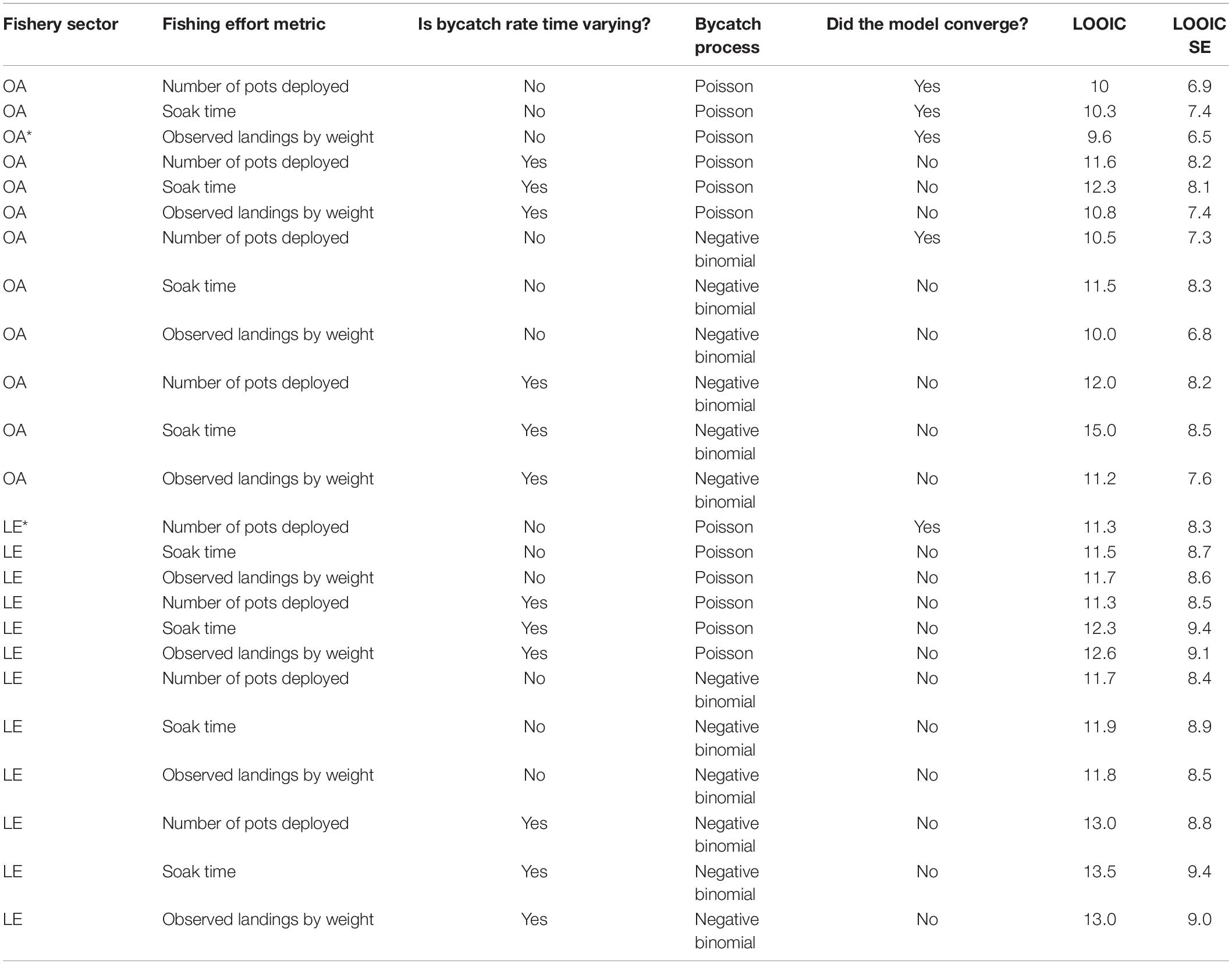
Table 1. Model diagnostics [convergence, LOOIC, and LOOIC standard error (SE)] by fishery sector for each fishing effort metric, time-varying, and bycatch process model choice. Asterisk (*) indicates the model that both converged and had the lowest LOOIC.

Humpback whales were observed entangled in United States West Coast sablefish pot gear twice by fishery observers since 2002. The single 2014 entanglement in the LE pot fishery led to an annual estimate in the most recent year of available data (2019) of 0.13 entanglements (95% CI: 0.0–1.0; Table 2). The single 2016 entanglement in the OA pot fishery led to a 2019 estimate of 1.02 entanglements (CI: 0.0–4.0; Table 3).

TABLE 2

Table 2. The data used to calculate humpback whale bycatch in the LE sablefish pot fishery collected by fishery observers (observed) and the estimated mean and 95% credible interval (CI: lower–upper) from the best model. The best model included a constant bycatch rate, a Poisson count process, and used the number of observed pots deployed as fishing effort.

TABLE 3

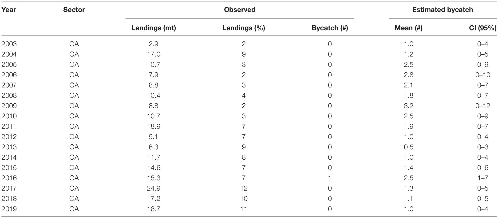
Table 3. The data used to calculate humpback whale bycatch in the OA sablefish pot fishery collected by fishery observers (observed) and the estimated mean and 95% credible interval (CI: lower–upper) from the best model. The best model included a constant bycatch rate, a Poisson count process, and used the total weight (mt) of landings from all trips that carried an observer (observed) as fishing effort.

The 2019 annual estimate of entanglements from the LE + OA sectors combined was 1.15 (CI: 0.0–5.0). This estimate was below both the 2012 and 2020 annual entanglement threshold (Figure 1 bottom panel; 2012: 3 whales/year; NMFS, 2012, 2020a: 5 whales/year; NMFS, 2020a). The most recent estimated 5-year average (2015–2019) of entanglements from the LE + OA sectors combined was 1.60 (CI: 0.2–4.8; Tables 2, 3 and Figure 1). This estimate was above the 2012 5-year average threshold of 1 animal/year (Figure 1 top panel; NMFS, 2012), but below the 2020 5-year average threshold of 2.34 animals/year (NMFS, 2020a; Figure 1 top panel). Exceeding the 2012 5-year average threshold contributed, in part, to the re-evaluation of the original 2012 Biological Opinion and resulted in the revised threshold value.

FIGURE 1

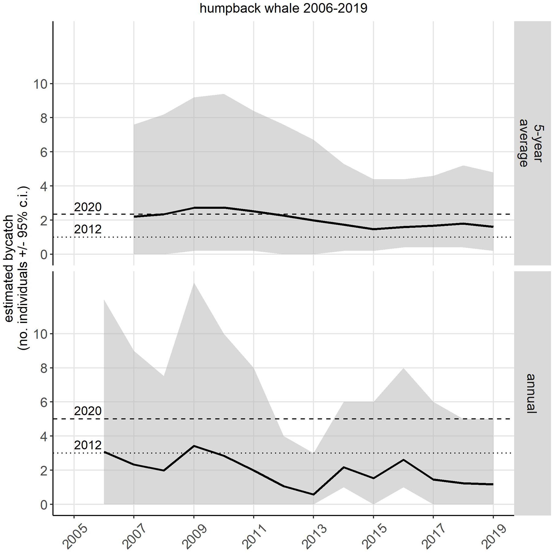
Figure 1. Estimated bycatch [number of individuals, 95% credible interval (CI)] of humpback whales in the United States West Coast sablefish pot fishery. Estimates were made for LE and OA sectors separately and then the estimates from the two sectors were summed. The two Biological Opinions (2012 and 2020) governing the incidental take of humpback whales in this fishery specified a 5-year average (top panel) in 2012 (dotted line) as 1 whale/year, and 2.34 whales/year in 2020. The specified annual take threshold (bottom panel) in 2012 (dotted line) was 3 whales/year and in 2020 (dashed line) was 5 whales/year.

Both the annual and the 5-year average estimated takes showed a peak in 2009, then trended downward until 2013 and then upward until 2017, after which the estimates level off (Figure 1). The probability of exceeding the thresholds follows a similar trend over time as the estimated takes and uncertainty, with the entire probability trend shifting location along the y-axis (probability) depending on the threshold (Figure 2). This results in the probability of exceeding the bycatch thresholds higher overall in 2012, when the thresholds were lower (three whales in a single year or a 5-year average of 1/year) as compared to the 2020 thresholds (five whales in a single year or a 5-year average of 2.34/year; Figure 2). Irrespective of the specific values of the threshold (e.g., 2012 vs. 2020), the probability of exceeding the 5-year average threshold appears to always be greater than the probability of exceeding the annual threshold (Figure 2).

FIGURE 2

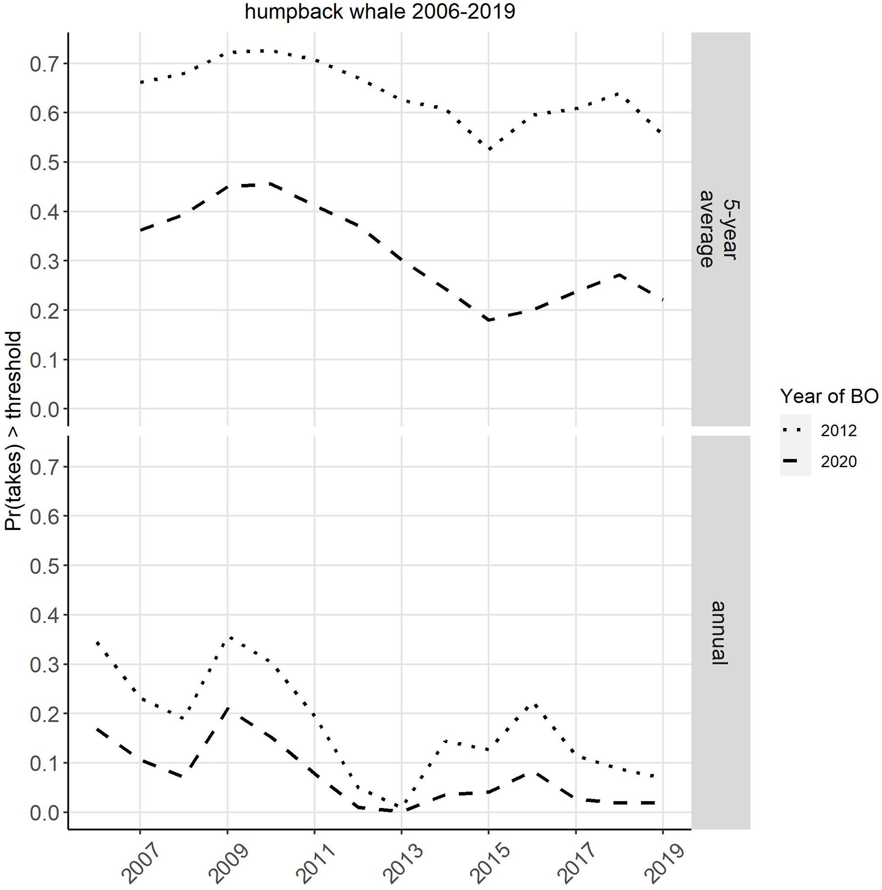
Figure 2. Probability of the 5-year average take estimate (top) or annual take estimate (bottom) exceeding the take threshold specified in the 2012 (dotted line) or 2020 (dashed line) Biological Opinion (BO) Incidental Take Statement. Currently these fisheries operate under the 2020 BO, which superseded the 2012 BO.

Sensitivity Analysis: Model Assumptions

Our simulation results highlight that with short time series (20 time steps) and sparse observations, data models that have more parameters than the Poisson are generally not supported (Figure 3). As expected, when data are generated from a Poisson model, the Poisson estimation model generally has the lowest LOOIC estimate, corresponding to more support for a Poisson bycatch process (Figure 3). This result was true regardless of the simulated bycatch rate, which controlled the sparsity in the data. Sparse and over-dispersed data from a negative binomial distribution is more challenging; with low mean bycatch rates (0.1), we found more support for zero-inflated Poisson models, whereas, at higher bycatch rates (1.0) the negative binomial model was favored (smaller changes in LOOIC; Figure 3). This indicates that the negative binomial model might not be the best choice for sparse datasets. A benefit of many Bayesian model selection tools, such as LOOIC, is that, in addition to individual point estimates, standard errors can also be estimated. As expected with short time series and sparse data, we found that for many of our simulated replicates, standard errors overlapped between models; the average difference in LOOIC between models was 1.98, and average standard error across all estimates was 8.16.

FIGURE 3

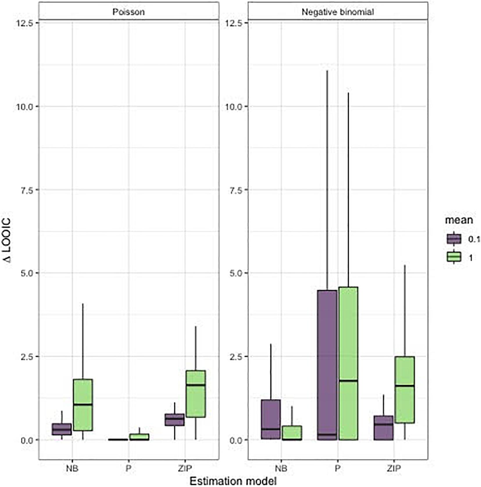
Figure 3. Distribution of LOOIC differences for our model selection applied to simulated time series. Each boxplot represents 100 time series generated from each level of the mean bycatch rate (0.1, 1), estimation model (“NB,” negative binomial; “P,” Poisson; “ZIP,” zero-inflated Poisson), and simulation model (Poisson, negative binomial).

Sensitivity Analysis: Data Assumptions

Using the depth breakpoints identified for each sector (Supplementary Figure 1; 395.5 m for LE sector and 360.0 m for OA sector), we repeated our analysis using a model with a Poisson distribution. Because the deep stratum for both sectors had no observed takes, we focused on results for the shallow stratum. Estimated observed bycatch rates for both sectors highlighted that the expected observed takes using all depths were very similar to expected observed takes using only the shallow depths where takes had been observed (Supplementary Figure 2). For the LE sector during the 2012–2013 period, estimates using all depths were slightly greater than using only the shallow depths, but these differences were because of a sharp reduction in retained catch in the shallow sector during this period (Supplementary Figure 1). The posterior distribution of total takes (observed + posterior predictive distribution of unobserved takes) was also similar between depth scenarios (Supplementary Figure 3). The LE sector estimates ranged from 0 to slightly more than 1 animal irrespective of the depth stratum and the OA sector estimates ranged from less than 1 to slightly more than 2.5 animals, irrespective of depth grouping (Supplementary Figure 3). In both sectors, estimates were largest in the years when observed takes occurred, again irrespective of the depth grouping (Supplementary Figure 3). The 5-year average of takes and probabilities of exceeding the 2020 5-year threshold of 2.34 takes/year (LE + OA) also appeared to be insensitive to the depth grouping, with similar trajectories in estimates from both depth scenarios (Supplementary Figure 4).

Discussion

This work demonstrates how Bayesian models can be used to estimate rare bycatch events: in this case, humpback whale entanglements in the United States West Coast sablefish pot fishery. This approach can more accurately estimate bycatch and uncertainty than other methods (e.g., ratio estimators; Lewin et al., 2010; Carretta and Moore, 2014; Martin et al., 2015) and yields probabilities for unobserved entanglements. Our simulations show that when data are rare but not over-dispersed, simpler bycatch-generating processes (i.e., Poisson) are favored over more complex distributions (e.g., negative binomial). However, as expected, when data are rare and over-dispersed, more complex distributions need to be employed, but the precise distribution depends on the sparsity of the data (e.g., zero-inflated vs. negative binomial). For 2019, the most recent estimates available, a Poisson process estimated a 5-year average of 1.60 entanglements/year for 2015–2019, for both sectors combined, which is less than the 2020 5-year average threshold of 2.34 entanglements/year. However, the uncertainty around that 5-year average estimate suggests that entanglements could be as high as 4.8/year. Our analysis also suggests that the results are not sensitive to assumptions about the data. Splitting the data by depth and comparing the model using all depths to the model using only the shallow depth stratum demonstrated that bycatch rates, posterior predictive distributions, and the probability of exceeding the 2020 threshold did not depend on these stratification choices.

The NMFS began using Bayesian models to estimate humpback whale bycatch in the United States West Coast sablefish pot fishery in 2019. That analysis resulted in estimates of humpback whale bycatch in the fishery that exceeded the previously anticipated bycatch limits, in part, contributing to a new review of the fishery and humpback bycatch risk under the ESA. While the California/Oregon/Washington stock showed long-term increases in abundance from 1990 to 2008, estimates from 2008 to 2014 suggest a period of leveling-off, but data from 2014 to 2018 suggest another period of population growth along the United States West Coast (Carretta et al., 2020b; Calambokidis and Barlow, 2020). The most recent Potential Biological Removal (PBR) for humpback whales in United States waters is 16.7 whales/year (Carretta et al., 2020b). Estimates of mortality in the LE sablefish pot fishery are generally less than one whale per year (Table 1), whereas estimates of humpback mortality from the OA Fixed Gear pot fishery are between one and three whale mortalities per year (Table 2). Together, these two fisheries represent about 10% of the total PBR.

The goal of the MMPA is to reduce incidental mortality and serious injury of all marine mammals to insignificant levels approaching a zero rate. This goal has been defined as the threshold for mortality and serious injury at 10% of PBR for a stock of marine mammals (69 FR 23477). As a result, we estimate that the mortality and serious injury associated with the sablefish pot fishery is approaching this threshold by itself, while numerous other sources of mortality and serious injury are also occurring associated with other fishery and non-fishery sources. For example, the number of confirmed humpback whale entanglements from all sources was on the rise from 16 confirmed entanglements in 2014 to 48 confirmed in 2016 (Santora and Lawson, 2021), coinciding with the time period in which the LE and OA sablefish pot fisheries each recorded a humpback whale entanglement. Since 2016, confirmed humpback whale entanglements have been between 17 and 34/year (Santora and Lawson, 2021).

Analytical Challenges

Despite the flexibility of the models presented here, there still remain several challenges and limitations to this method. For the two sectors presented here, we were able to successfully compare models in terms of bycatch rates (time-varying vs. constant) and some processes (Poisson vs. negative binomial). However, this is unlikely to always be the case, and indeed we were unable to compare all possible processes (e.g., zero-inflated) using the humpback data and have encountered other rare bycatch modeling scenarios where direct comparison was impossible as none of the models passed the diagnostic criteria (Jannot et al., 2021). In the case where all models failed, yet bycatch estimates were still required for management purposes, we chose the simplest form of the models (constant rate, Poisson) and compared among effort metrics (Jannot et al., 2021). None-the-less, the specific nature of the data sparsity and dispersion can hamper the optimal performance of the models and limit our understanding of bycatch.

Another limitation of this method is the nature of the data itself. In the examples we have provided, we rely almost exclusively on observer data. In the LE and OA sectors presented here, we have a plethora of information from observed vessels that could provide insight into bycatch, such as multiple proxy metrics of fishing effort (# pots, weight of landed catch), depth, latitude, and duration as well as others. However, we have much less comparable data from the unobserved portion of the fleet which limits our understanding of the causes of bycatch, because, for example, we have to assume that the fishing depth distribution is similar among observed and unobserved vessels. The “observer effect” posits that observed vessels can behave quite differently than unobserved vessels (Hilborn et al., 2009; Faunce and Barbeaux, 2011). Therefore, any inferences about humpback whale bycatch must be tempered by the limited data available from unobserved vessels and the potential for an observer effect.

Fisheries that are similar but have no observed recorded takes also pose a challenge to this method. As mentioned above, there is a third pot sector, the CS pot fishery. Since 2011, this fishery has had 100% monitoring of catch at-sea. During 2011–2014 all CS pot fishery trips were monitored by fisheries observers. Since 2015, while all trips are monitored, only roughly 50% of trips have been monitored by observers and the remainder of trips are monitored by EM (Somers et al., 2020a). To date, the CS pot fishery has not recorded a humpback whale entangled in pot gear since the fishery inception in 2011. Despite the fishery being 100% monitored, there might still be unaccounted for bycatch. For example, a humpback whale could become entangled in pot gear while the gear was fishing, but unattended, and then swim away with gear attached and therefore, be unobserved and undocumented, which is a plausible scenario (see section “Unobserved Bycatch and Cryptic Mortality”). To estimate bycatch in the CS fishery, we would have to assume that bycatch rates are shared from either the LE or the OA fishery, either by taking an average across the sectors, or using a more precautionary approach, assuming the higher of the two bycatch rates. While the gear used (pots, lines, and floats) in the CS pot fishery is similar to the gear used in the LE and OA fisheries, CS vessels do not fish precisely the same as either fleet. For example, the LE fleet targets sablefish during a season (April–October) whereas the CS fleet can fish all year. In terms of fishing effort, CS vessels generally deploy similar numbers of pots as LE vessels, which is more pots per gear deployment than OA vessels. Also the CS fleet holds quota for other species besides groundfish, whereas the LE and OA fleets can only land other groundfish up to species-specific trip limits. In this way, the problem is analogous to the observer effect, to make estimates for the CS fleet, we would have to make untested assumptions about fishing effort and the manner in which pots are fished in the CS fleet based on information from the LE or OA fleet.

Unobserved Bycatch and Cryptic Mortality

One of the advantages to the method we present here is that it accounts for unobserved entanglements. Estimating unobserved entanglements is particularly important in the case of west coast humpback whales. Observers do not detect all humpback whales that have been entangled in sablefish pot gear, given that whales entangled in this gear type have been opportunistically reported at various locations off the west coast (Saez et al., 2021). Entanglements might go unobserved for multiple reasons. For example, observers may not be present on a trip when an entanglement occurs (only a portion of trips are observed; Tables 1, 2). Whales could break free of the entanglement before observation (Saez et al., 2021), and entangled whales could then leave the fishing area with gear attached. In all three sectors (LE, OA, and CS), it is common for vessels (with or without observers present) to deploy gear at the fishing grounds and then leave the area to let the gear fish. OA pot vessels very often place the gear in a single location and then return throughout the year during days of good weather to retrieve the catch, resetting the gear back to its original location. In these cases, the gear is fishing unattended for a period of time, which can vary from a few hours or days potentially up to weeks (a.k.a. soak time). During these long soak times, whales could become entangled in gear and swim away without being observed.

Between 2006 and 2017, there were five confirmed reports of humpback entanglements with sablefish pot gear (Saez et al., 2021). These five observations are considered a minimum estimate, due to the opportunistic nature of reporting at-sea entanglements. These opportunistic observations are likely biased because they are not a random selection of observations in space or time. Thus, these observations cannot be directly incorporated into the models presented here. A total of 17 opportunistic records of humpback whale entanglements in fishing gear were reported in 2019. In the 2020 Biological Opinion, a very small percentage (less than 5%) of entanglements from 2011 to 2019 that were attributed to a fishery were associated with sablefish pot gear (NMFS, 2020a). Seven of the 17 reports could be attributed to a fishery but none (0) of those were associated with sablefish gear. The remaining 10 entanglement reports could not be attributed to a specific fishery. Based on this information, we assume that no more than one of the 10 entanglements with unidentified fishing gear would be expected to be associated with sablefish gear. The Bayesian framework generates posterior predictive distributions for unobserved entanglements in addition to estimates and associated uncertainty for observed entanglements. Therefore, estimates from these models do account for these unobserved entanglements.

Assessing the number of unobserved pot or trap gear entanglements of humpback whales from any fishery on the United States West Coast is difficult due to the nature of opportunistic reports (i.e., non-random) and the rarity of systematically observed incidents (human or EM). Undetected, a.k.a., cryptic, injury and mortality of marine mammals is challenging to estimate, but progress has been made for several populations (Williams et al., 2011; Peltier et al., 2012; Prado et al., 2013; Wells et al., 2015; Carretta et al., 2016; Young et al., 2019; Harting et al., 2021; Pace et al., 2021). Marine mammal carcass recovery rates (= detection rates) have been estimated with several approaches: tracking the fate of known individuals over time (Wells et al., 2015); combining abundance estimates and estimated annual survival in Monte Carlo simulations to estimate carcass numbers available for detection (Carretta et al., 2016; Harting et al., 2021), comparing observed stranding numbers to estimated mortalities from population models (Pace et al., 2021), comparing numbers of marked carcasses at sea with those arriving ashore (Prado et al., 2013) and using drift models to estimate the fraction of carcasses arriving ashore (Peltier et al., 2012; Young et al., 2019). Generally, published estimates of carcass recovery rates are quite low, ranging from near-zero for some pelagic species such as killer whales and false killer whales (Williams et al., 2011), <10% for common dolphins (Peltier et al., 2012), 33% for an embayment population of coastal bottlenose dolphins (Wells et al., 2015), 36% for North Atlantic right whales (Pace et al., 2021), and 46% for Hawaiian monk seals (Harting et al., 2021). Most species lack estimates of undetected mortality and serious injury and, for pelagic species, at-sea sightings and strandings provide minimum accounting of human-related mortality and serious injury due to low probabilities of stranding and detection (Faerber and Baird, 2010; Williams et al., 2011).

Our bycatch model includes estimates of interactions in unobserved portions of the sablefish fishery, but both observed and modeled interaction rates are based on time windows when observers are present. These interaction rates may be negatively biased because they exclude unobserved cases where whales swam off with gear and subsequently incur serious injury or die from chronic entanglement over a period of months (Moore and van der Hoop, 2012). Estimates of interaction rates also exclude unobserved cases of whales becoming entangled in lost gear, which is a special case of “fishing effort” outside the purview of observer programs. Baseline data on levels of lost gear generally shows that <2% of pot gear is lost (Supplementary Table 1), but assessment of how and why gear is lost (rough weather vs. whales swimming away with gear) is difficult.

Other United States West Coast Fisheries

From 2011 to 2019, NMFS received and evaluated 170 separate confirmed humpback whale entanglement reports from the United States West Coast (excluding re-sightings; NMFS, 2019; NWFSC, 2020b; Saez et al., 2021). With the limited exception of a few reports from fishery observers, including the two reports from sablefish fishery observers assessed here, most of these reports are products of opportunistic, i.e., non-random, sightings, and reportings from sources that include marine mammal stranding and response networks, members of the public, United States Coast Guard, law enforcement agencies, and marine researchers. Given that the majority of entanglement reports are opportunistic, NMFS assumes that many large whale entanglements are not observed or, if observed, are not likely to be reported except as required by fisheries observers or EM programs. Therefore, it is likely that reports of large whale entanglements represent an unknown fraction of the total number of whales that have been entangled over time (Saez et al., 2021). Currently, the number of total whale entanglements that occur along the United States West Coast relative to the number of entanglements reported is unknown (Saez et al., 2021). However, rope scarring from entanglements with fishing gear are evident on one third to one half of all humpback whales (Calambokidis et al., 2008), which may provide insight on the total number of whales that have been entangled at least once.

Numerous other United States West Coast commercial and recreational fisheries have been associated with the origins of whale entanglements reported through opportunistic sources, including Dungeness crab, spot prawn, spiny lobster, and rock crab pot or trap fisheries, along with various set and drift gillnet fisheries (Saez et al., 2021). A cursory review of the literature provided no other examples of the use of this method in fixed gear fisheries to estimate large whale bycatch. Many of these fisheries do not employ use of fishery monitoring schemes like the sablefish pot fishery presented here. Unobserved fisheries pose a challenge to estimating large whale bycatch. The Bayesian method we present here relies on systematically collected random samples of lethal entanglements in fishing gear, a measure of observation effort, and a measure of total fishing effort for the entire fleet. For the United States West Coast sablefish pot fishery we used data from fishery monitoring programs (e.g., human observers and EM) that systematically collect data on whale entanglements. For unmonitored fisheries, observed bycatch rates (θ) could be borrowed from observed fisheries and applied to unobserved fisheries. However, this would require having some measure of observed effort for the entanglements (E_y) which is unlikely in unmonitored fisheries. In many unmonitored fisheries, the only available data will be a count of entanglements reported and some measure of total fishing effort (number of: vessels, gear deployments, pot or traps; gear soak time; and total fleet landings). Entanglement estimates in most cases will not be collected systematically and therefore not related to observational effort in any meaningful way, making the Bayesian method presented here less than ideal for unmonitored fisheries. However, one case where our method might prove useful are species such as the North Atlantic right whale, where a large proportion of the population has been observed and identified by photograph (Knowlton et al., 2012). In theory, if observation and entanglement rates could be constructed from photographs (Knowlton et al., 2012) and entangling gear appropriately assigned to a fishery with available data on fishing effort, then bycatch estimates could be obtained for that fishery.

Conclusion

Large whale entanglement and bycatch in fishing gear presents a challenge to analysts and managers that need to estimate the number of, and mitigate for, these low frequency events. Currently, the most robust data estimates of whale entanglements mainly comes from at-sea fishery observers or EM devices. However, not all fisheries are monitored and for those fisheries that are monitored, it is often the case that not all vessels within a fishery are observed. The Bayesian method used here provides robust estimates of both observed and unobserved bycatch in partially monitored fisheries, thus overcoming some of the challenges posed by rare event data. This method is flexible and can be used on a wide-variety of commonly used generalized linear models and provides reasonable estimates of uncertainty around bycatch estimates as well as accounting for undetected bycatch by providing estimates of bycatch when the observed estimate is zero. More work needs to be done to develop methods that use non-random opportunistic observations of whale entanglement. However, the Bayesian time-series used here provides managers and analysts with an important tool to accurately assess the impacts of fishing on large whales.

Data Availability Statement

The datasets presented in this article are not readily available because of the confidential nature of the NOAA west coast sablefish fishery observer data. All data to replicate our analyses is included in the tables in the article, and code is provided via our public R package. The raw data (e.g., at the level of individual sets) for the case studies presented here are only available upon request from the NOAA NWFSC FOS Program. Requests to access the datasets should be directed to JJ, jason.jannot@noaa.gov.

Author Contributions

JJ and EW conceptualized the study, conducted the analyses, and created the tables and figures. JJ and KS prepared, processed, and summarized the data. JJ and EW wrote the manuscript with contributions from KS, BF, TG, DL, and JC. All authors contributed to manuscript revision, and read and approved the submitted version.

Funding

NOAA Fisheries Northwest Fisheries Science Center supported JJ, EW, KS, BF, and TG. NOAA Fisheries West Coast Regional Office supported DL. NOAA Fisheries Southwest Fisheries Science Center supported JC. Funding from the Northwest Fisheries Science Center Fisheries Observation Science Program and Conservation Biology Division were used for publication fees.

Conflict of Interest

The authors declare that the research was conducted in the absence of any commercial or financial relationships that could be construed as a potential conflict of interest.

Publisher’s Note

All claims expressed in this article are solely those of the authors and do not necessarily represent those of their affiliated organizations, or those of the publisher, the editors and the reviewers. Any product that may be evaluated in this article, or claim that may be made by its manufacturer, is not guaranteed or endorsed by the publisher.

Acknowledgments

We gratefully acknowledge the hard work and dedication of observers from the West Coast Groundfish Observer Program and the At-Sea Hake Observer Program, as well as contributions from observer program staff. We would like to thank the NOAA West Coast Strandings Network Coordinators: Kristin Wilkinson, Brent Norberg, Justin Viezbicke, and Justin Greenman for providing strandings data. We would also like to thank Jameal Samhouri and three reviewers for constructive comments on earlier versions of this manuscript.

Supplementary Material

The Supplementary Material for this article can be found online at: https://www.frontiersin.org/articles/10.3389/fmars.2021.775187/full#supplementary-material

Footnotes

1. ^ https://ericward-noaa.github.io/bycatch/

References

Amande, M. J., Chassot, E., Chavance, P., Murua, H., De Molina, A. D., and Bez, N. (2012). Precision in bycatch estimates: the case of tuna purse-seine fisheries in the Indian Ocean. ICES J. Mar. Sci. 69, 1501–1510. doi: 10.1093/icesjms/fss106

CrossRef Full Text | Google Scholar

Babcock, E. A., Pikitch, E. K., and Hudson, C. G. (2003). How much Observer Coverage is Enough to Adequately Estimate Bycatch?. Washington, DC: Pew Institute for Ocean Science and Oceana. doi: 10.1111/j.1748-7692.2010.00444.x

CrossRef Full Text | Google Scholar

Bettridge, S. O. M., Baker, C. S., Barlow, J., Clapham, P., Ford, M. J., Gouveia, D., et al. (2015). Status Review of the Humpback Whale (Megaptera novaeangliae) Under the Endangered Species Act. La Jolla, CA: U. S. Department Of Commerce.

Google Scholar

Borges, L., Zuur, A. R., Rogan, E., and Officer, R. (2005). Choosing the best sampling unit and auxiliary variable for discards estimations. Fish. Res. 75, 29–39. doi: 10.1016/j.fishres.2005.05.002

CrossRef Full Text | Google Scholar

Breiman, L. (2001). Statistical modeling: the two cultures (with comments and a rejoinder by the author). J. Stat. Sci. 19:133. doi: 10.1214/ss/1009213726

CrossRef Full Text | Google Scholar

Calambokidis, J., and Barlow, J. (2020). Updated Abundance Estimates for Blue and Humpback Whales Along the U.S. West Coast using data through 2018. NOAA Technical Memorandum NMFS-SWFSC-634. La Jolla, CA: U.S. Department of Commerce.

Google Scholar

Calambokidis, J., Falcone, E. A., Quinn, T. J., Burdin, A. M., Clapham, P. J., Ford, J. K. B., et al. (2008). SPLASH: Structure of Populations, Levels of Abundance and Status of Humpback Whales in the North Pacific. Seattle, WA: U.S. Dept of Commerce - Western Administrative Center, 57.

Google Scholar

Carretta, J. V., Danil, K., Chivers, S. J., Weller, D. W., Janiger, D. S., Berman-Kowalewski, M., et al. (2016). Recovery rates of bottlenose dolphin (Tursiops truncatus) carcasses estimated from stranding and survival rate data. Mar. Mamm. Sci. 32, 349–362. doi: 10.1111/mms.12264

CrossRef Full Text | Google Scholar

Carretta, J. V., Delean, B., Helker, V. T., Muto, M., Greenman, J., Wilkinson, K. M., et al. (2020a). Sources of Human-Related Injury and Mortality for U.S. Pacific West Coast Marine Mammal Stock Assessments, 2014-2018. NOAA Tech. Memo. NOAA-TM-NMFS-SWFSC-631. La Jolla, CA.

Google Scholar

Carretta, J. V., Forney, K. A., Oleson, E. M., Weller, D. W., Lang, A. R., Baker, J., et al. (2020b). U.S. Pacific Marine Mammal Stock Assessments: 2019. NOAA Tech. Memo. NOAA-TM-NMFS-SWFSC-629. La Jolla, CA.

Google Scholar

Carretta, J. V., and Moore, J. E. (2014). Recommendations for Pooling Annual Bycatch Estimates When Events are Rare. NOAA Tech. Memo. NOAA-TM-NMFS-SWFSC-528. La Jolla, CA.

Google Scholar

Carretta, J. V., Moore, J. E., and Forney, K. A. (2017). Regression Tree and Ratio Estimates of Marine Mammal, Sea Turtle, and Seabird Bycatch in the California Drift Gillnet Fishery, 1990-2015. NOAA Tech. Memo. NOAA-TM-NMFS-SWFSC-568. La Jolla, CA.

Google Scholar

Cosandey-Godin, A., Krainski, E. T., Worm, B., and Flemming, J. M. (2015). Applying Bayesian spatiotemporal models to fisheries bycatch in the Canadian Arctic. Can. J. Fish. Aquat. Sci. 72, 186–197.

Google Scholar

Curtis, K. A., and Carretta, J. V. (2020). ObsCovgTools: assessing observer coverage needed to document and estimate rare event bycatch. Fish. Res. 225:105493. doi: 10.1016/j.fishres.2020.105493

CrossRef Full Text | Google Scholar

Dixon, P. M., Ellison, A. M., and Gotelli, N. J. (2005). Improving the precision of estimates of the frequency of rare events. Ecology 86, 1114–1123. doi: 10.1890/04-0601

CrossRef Full Text | Google Scholar

Faerber, M. M., and Baird, R. W. (2010). Does a lack of observed beaked whale strandings in military exercise areas mean no impacts have occurred? A comparison of stranding and detection probabilities in the Canary and main Hawaiian Islands. Mar. Mamm. Sci. 26, 602–613. doi: 10.1111/j.1748-7692.2010.00370.x

CrossRef Full Text | Google Scholar

Faunce, C. H., and Barbeaux, S. J. (2011). The frequency and quantity of Alaskan groundfish catcher-vessel landings made with and without an observer. ICES J. Mar. Sci. 68, 1757–1763. doi: 10.1093/icesjms/fsr090

CrossRef Full Text | Google Scholar

Gilman, E., Suuronen, P., Hall, M., and Kennelly, S. (2013). Causes and methods to estimate cryptic sources of fishing mortality. Fish. Biol. 83, 766–803. doi: 10.1111/jfb.12148

PubMed Abstract | CrossRef Full Text | Google Scholar

Harting, A. L., Barbieri, M. M., Baker, J. D., Mercer, T. A., Johanos, T. C., Robinson, S. J., et al. (2021). Population-level impacts of natural and anthropogenic causes-of-death for Hawaiian monk seals in the main Hawaiian Islands. Mar. Mamm. Sci. 37, 235–250. doi: 10.1111/mms.12742

CrossRef Full Text | Google Scholar

Hennig, C. (2020). fpc: Flexible Procedures for Clustering. R Package Version 2.2-9. Available online at: https://CRAN.R-project.org/package=fpc (accessed December 06, 2020).

Google Scholar

Hilborn, R., Benoît, H. P., and Allard, J. (2009). Can the data from at-sea observer surveys be used to make general inferences about catch composition and discards? Can. J. Fish. Aquatic Sci. 66, 2025–2039. doi: 10.1139/F09-116

PubMed Abstract | CrossRef Full Text | Google Scholar

Jannot, J. E., Wuest, A., Good, T. P., Somers, K. A., Tuttle, V. J., Richerson, K. E., et al. (2021). Seabird Bycatch in U.S. West Coast Fisheries, 2002–18. NOAA Technical Memorandum NMFS-NWFSC-165. Seattle, WA: U.S. Department of Commerce.

Google Scholar

Knowlton, A. R., Hamilton, P. K., Marx, M. K., Pettis, H. M., and Kraus, S. D. (2012). Monitoring North Atlantic right whale Eubalaena glacialis entanglement rates: a 30 yr. retrospective. Mar. Ecol. Prog. Ser. 466, 293–302. doi: 10.3354/meps09923

CrossRef Full Text | Google Scholar

Komoroske, L. M., and Lewison, R. L. (2015). Addressing fisheries bycatch in a changing world. Front. Mar. Sci. 2:83. doi: 10.3389/fmars.2015.00083

CrossRef Full Text | Google Scholar

Lewin, W.-C., Freyhof, J., Huckstorf, V., Mehner, T., and Wolter, C. (2010). When no catches matter: coping with zeros in environmental assessments. Ecol. Indic. 10, 572–583. doi: 10.1016/j.ecolind.2009.09.006

CrossRef Full Text | Google Scholar

Martin, S. L., Stohs, S. M., and Moore, J. E. (2015). Bayesian inference and assessment for rare-event bycatch in marine fisheries: a drift gillnet fishery case study. Ecol. Appl. 25, 416–429. doi: 10.1890/14-0059.1

CrossRef Full Text | Google Scholar

McCracken, M. L. (2004). Modeling a Very Rare Event to Estimate Sea Turtle Bycatch Lessons Learned. NOAA Tech. Memo. NMFS-PIFSC-3. Honolulu, HI.

Google Scholar

Moore, J. E., Curtis, K. A., Lewison, R. L., Dillingham, P. W., Cope, J. M., Fordham, S. V., et al. (2013). Evaluating sustainability of fisheries bycatch mortality for marine megafauna: a review of conservation reference points for data-limited populations. Environ. Conserv. 40, 329–344. doi: 10.1017/S037689291300012X

CrossRef Full Text | Google Scholar

Moore, J. E., Merrick, R. L., Barlow, J., Bettridge, S. O. M., Carretta, J. V., Eagle, T. C., et al. (2011). Guidelines for Assessing Marine Mammal Stocks: Report of the GAMMS III Workshop, February 15-18, 2011. La Jolla, CA: National Marine Fisheries Service.

Google Scholar

Moore, M. J., and van der Hoop, J. M. (2012). The painful side of trap and fixed net fisheries: chronic entanglement of large whales. J. Mar. Sci. 2012:230653. doi: 10.1155/2012/230653

CrossRef Full Text | Google Scholar

NMFS (1991). Final Recovery Plan for the Humpback Whale (Megaptera novaeangliae). Prepared by the Humpback Whale Recovery Team for the National Marine Fisheries Service. Silver Spring, MD: National Marine Fisheries Service, 105.

Google Scholar

NMFS (2004). Evaluating bycatch: A National Approach to Standardized Bycatch Monitoring Programs. NOAA Tech. Memo. NMFSF/SPO-66. Silver Springs, MD: U.S. Department of Commerce, 108.

Google Scholar

NMFS (2012). Endangered Species Act (ESA) Section 7(a)(2) Biological and Section 7(a)(2) “Not Likely to Adversely Affect” Determination Continuing Operation of the Pacific Coast Groundfish Fishery. West Coast Region: National Marine Fisheries Service.

Google Scholar

NMFS (2019). 2018 West Coast Whale Entanglement Report. Spring 2019. Long Beach, CA: NOAA Fisheries West Coast Region, 10.

Google Scholar

NMFS (2020a). Endangered Species Act (ESA) Section 7(a)(2) Biological and Conference Opinion Continuing Operation of the Pacific Coast Groundfish Fishery. West Coast Region: National Marine Fisheries Service.

Google Scholar

NMFS (2020b). 2019 West Coast Whale Entanglement Summary. Spring 2020. Long Beach, CA: NOAA Fisheries West Coast Region, 4.

Google Scholar

NWFSC (2020c). Training Manual West Coast Groundfish Observer Program. Seattle, WA: Northwest Fisheries Science Center.

Google Scholar

Pace, R. M. III, Williams, R., Kraus, S. D., Knowlton, A. R., and Pettis, H. M. (2021). Cryptic mortality of North Atlantic right whales. Conserv. Sci. Pract. 3:e346. doi: 10.1111/csp2.346

CrossRef Full Text | Google Scholar

Parsa, M., Emery, T. J., Williams, A. J., and Nicol, S. (2020). An empirical Bayesian approach for estimating fleet- and vessel-level bycatch rates in fisheries with effort heterogeneity and limited data: a prospective tool for measuring bycatch mitigation performance. ICES J. Mar. Sci. 77, 921–929. doi: 10.1093/icesjms/fsaa020

CrossRef Full Text | Google Scholar

Peltier, H., Dabin, W., Daniel, P., Van Canneyt, O., Dorémus, G., Huon, M., et al. (2012). The significance of stranding data as indicators of cetacean populations at sea: modelling the drift of cetacean carcasses. Ecol. Indic. 18, 278–290. doi: 10.1016/j.ecolind.2011.11.014

CrossRef Full Text | Google Scholar

Prado, J. H. F., Secchi, E. R., and Kinas, P. G. (2013). Mark-recapture of the endangered franciscana dolphin (Pontoporia blainvillei) killed in gillnet fisheries to estimate past bycatch from time series of stranded carcasses in southern Brazil. Ecol. Indic. 32, 35–41. doi: 10.1016/j.ecolind.2013.03.005

CrossRef Full Text | Google Scholar

R Core Team (2020). R: A Language and Environment for Statistical Computing. Vienna: R Foundation for Statistical Computing.

Google Scholar

Rochet, M. J., and Trenkel, V. M. (2005). Factors for the variability of discards: assumptions and field evidence. Can. J. Fish. Aquatic Sci. 62, 224–235. doi: 10.1139/f04-185

PubMed Abstract | CrossRef Full Text | Google Scholar

Saez, L., Lawson, D., and DeAngelis, M. L. (2021). Large whale Entanglements off the U.S. West Coast, from 1982-2017. Silver Spring, MD: United States Department of Commerce, 50.

Google Scholar

Santora, J., and Lawson, D. (2021). IEA Integrated Ecosystem Assessment California Current Integrated Ecosystem Assessment Ecosystem Context for Reducing West Coast Whale Entanglements California Current Project [Online]. Available online at: https://www.integratedecosystemassessment.noaa.gov/regions/california-current/cc-projects-whale-entanglement (accessed August 30, 2021)

Google Scholar

Siders, Z. A., Ducharme-Barth, N. D., Carvalho, F., Kobayashi, D., Martin, S., Raynor, J., et al. (2020). Ensemble random forests as a tool for modeling rare occurrences. Endang. Species Res. 43, 183–197. doi: 10.3354/esr01060

CrossRef Full Text | Google Scholar

Somers, K. A., Jannot, J. E., Richerson, K., Tuttle, V. J., and Mcveigh, J. (2020a). Fisheries Observation Science Program Coverage Rates, 2002-19. U.S. Dep. Commer. NOAA Data Report NMFS-NWFSC-DR-2020-03. Seattle, WA.

Google Scholar

Somers, K. A., Whitmire, C. E., Richerson, K., Jannot, J. E., Tuttle, V. J., and Mcveigh, J. (2020b). Fishing Effort in the 2002-17 Pacific Coast Groundfish Fisheries. NOAA Technical Memorandum NMFS-NWFSC-153. Seattle, WA.

Google Scholar

Stan Development Team (2021). Stan Modeling Language Users Guide and Reference Manual, 2.27. Available online at: https://mc-stan.org.

Google Scholar

Stock, B. C., Ward, E. J., Eguchi, T., Jannot, J. E., Thorson, J. T., Feist, B. E., et al. (2020). Comparing predictions of fisheries bycatch using multiple spatiotemporal species distribution model frameworks. Can. J. Fish. Aquatic Sci. 77, 146–163. doi: 10.1139/cjfas-2018-0281

PubMed Abstract | CrossRef Full Text | Google Scholar

Stratoudakis, Y., Fryer, R., Cook, R., and Pierce, G. (1999). Fish discarded from Scottish demersal vessels: estimators of total discards and annual estimates for targeted gadoids. ICES J. Mar. Sci. 56:592. doi: 10.1006/jmsc.1999.0500

CrossRef Full Text | Google Scholar

Vehtari, A., Gabry, J., Magnusson, M., Yao, Y., Bürkner, P., Paananen, T., et al. (2020). “loo: Efficient leave-one-out cross-validation and WAIC for Bayesian models”. R package version 2.2.0.

Google Scholar

Vehtari, A., Simpson, D., Gelman, A., Yao, Y., and Gabry, J. (2019). Pareto smoothed importance sampling. arXiv [Preprint] arXiv:1507.02646,

Google Scholar

Wade, P. R. (1998). Calculating limits to the allowable human-caused mortality of cetaceans and pinnipeds. Mar. Mamm. Sci. 14, 1–37. doi: 10.1111/j.1748-7692.1998.tb00688.x

CrossRef Full Text | Google Scholar

Wakefield, C. B., Hesp, S. A., Blight, S., Molony, B. W., Newman, S. J., and Hall, N. G. (2018). Uncertainty associated with total bycatch estimates for rarely-encountered species varies substantially with observer coverage levels: informing minimum requirements for statutory logbook validation. Mar. Policy 95, 273–282. doi: 10.1016/j.marpol.2018.05.018

CrossRef Full Text | Google Scholar

Walmsley, S., Leslie, R., and Sauer, W. (2007). Bycatch and discarding in the South African demersal trawl fishery. Fish. Res. 86, 15–30. doi: 10.1016/j.fishres.2007.03.002

CrossRef Full Text | Google Scholar

Ward, E., and Jannot, J. (2021). bycatch: Using Bayesian Generalized Linear Models for Estimating bycatch Rates and Generating Fleet-Level Expansions R Package (v1.0.6). Zenodo. doi: 10.5281/zenodo.4743823

CrossRef Full Text | Google Scholar

Wells, R. S., Allen, J. B., Lovewell, G., Gorzelany, J., Delynn, R. E., Fauquier, D. A., et al. (2015). Carcass-recovery rates for resident bottlenose dolphins in Sarasota Bay, Florida. Mar. Mamm. Sci. 31, 355–368. doi: 10.1111/mms.12142

CrossRef Full Text | Google Scholar

Wickham, H. (2016). ggplot2: Elegant Graphics for Data Analysis. New York, NY: Springer-Verlag. doi: 10.1007/978-3-319-24277-4

CrossRef Full Text | Google Scholar

Wickham, H., Averick, M., Bryan, J., Chang, W., Mcgowan, L. D., François, R., et al. (2019). Welcome to the tidyverse. J. Open Source Softw. 4:1686. doi: 10.21105/joss.01686

CrossRef Full Text | Google Scholar

Williams, R., Gero, S., Bejder, L., Calambokidis, J., Kraus, S. D., Lusseau, D., et al. (2011). Underestimating the damage: interpreting cetacean carcass recoveries in the context of the Deepwater Horizon/BP incident. Conserv. Lett. 4, 228–233. doi: 10.1111/j.1755-263X.2011.00168.x

CrossRef Full Text | Google Scholar

Young, C., Eguchi, T., Ames, J. A., Staedler, M., Hatfield, B. B., Harris, M., et al. (2019). Drift and beaching patterns of sea otter carcasses and car tire dummies. Mar. Mamm. Sci. 35, 1512–1526. doi: 10.1111/mms.12609

CrossRef Full Text | Google Scholar