Comparing Calibration Algorithms for the Rapid Characterization of Pretreated Corn Stover Using Near-Infrared Spectroscopy

Rapid characterization of biomass composition is a key enabling technology for biorefineries—the ability to measure the chemical composition of biomass materials entering the biorefinery as well as the composition of key process intermediate streams would allow real-time process control and the development of robust models to predict process performance. The utility of near-infrared (NIR) spectroscopy for rapid characterization requires multivariate algorithms for building calibration models. The most prevalent algorithm used for building calibration models using NIR spectra is the linear modeling algorithm Partial Least Squares Regression (PLS). Nonlinear regression algorithms (which are typically more computationally intensive than linear modeling approaches) have gained popularity in recent years due to their ability to solve a wide variety of classification and regression problems and the dramatic increase in available computational resources. In this work, we demonstrate that a calibration model can predict the composition of corn stover process intermediate samples pretreated with three different treatments—hot water (HW), dilute acid (DA), and deacetylation followed by dilute acid (DDA). We quantitatively compare three different algorithms for building prediction models based on near-infrared spectroscopy—partial least squares (PLS), support vector machines (SVM), and random forests (RF). We demonstrate the utility of improving model performance by accounting for instrument performance variability using repeated measurements of standard materials (e.g., the “repeatability file” strategy) and investigate its performance with nonlinear regression techniques, and we discuss methods for quantifying the uncertainties of specific predictions among the three methods.

1 Introduction

Rapid characterization of biomass composition is a key enabling technology for biorefineries—the ability to measure the chemical composition of biomass materials entering the biorefinery as well as the composition of key process intermediate streams would allow real-time process control and the development of robust models to predict process performance. There is substantial literature on the use of spectroscopic methods such as near-infrared (NIR) spectroscopy for rapid biomass characterization going back several decades (Abrams et al., 1987; Sanderson et al., 1996; Kelley et al., 2002; Tsuchikawa, 2007; Labbe et al., 2008; Tsuchikawa and Kobori, 2015) and including some comprehensive reviews (Xiao et al., 2014; Skvaril et al., 2017).

The use of NIR spectroscopy for rapid characterization requires multivariate algorithms for building calibration models (Höskuldsson, 1988; Beebe et al., 1998; Pasquini, 2018). The most prevalent algorithm used for building calibration models using NIR spectra is Partial Least Squares Regression (PLS). PLS is an extension of multiple linear regression and uses feature extraction to produce new latent variables (principal components) composed of linear combinations of the original variables that describe the majority of the variance correlated with the outcome of interest (Höskuldsson, 1988). While originally developed for the field of econometrics, PLS has been used in chemometrics since the 1970s, and is currently a standard method for NIRS regression (Geladi and Kowalski, 1986).

Nonlinear regression techniques have demonstrated utility in solving a wide variety of classification and prediction problems. In recent years their usage has increased due to a combination of dramatically increased availability of high-performance computing (HPC) tools and access to open-source implementation of these algorithms in computing languages such as R and Python. Support Vector Machines (SVM) (Awad and Khanna, 2015) and Random Forest (RF) (Breiman, 2001; Fawagreh et al., 2014) are two such nonlinear machine learning techniques. SVM regression expands upon the support vector machine classification technique (Cristianini and Shawe-Taylor, 2000) to fit a hyperplane that minimizes the residuals outside a defined error margin (ε-margin). In the training process, a cost parameter, C, is chosen, which defines the penalty for residuals above a certain value. SVM can be used to explain linear and nonlinear relationships through the use of kernel functions (Cristianini and Shawe-Taylor, 2000; Awad and Khanna, 2015). Radial bias functions (RBF) are often used with training sets having nonlinear relationships between dependent and independent variables. RBF functions require the additional tuning of the parameter σ, which controls for the level of nonlinearity in the model. Random Forest Modeling develops individual decision trees based on a randomly chosen selection of predictors and then aggregates tree results to determine the outcome of interest. The user must decide upon the number of predictors to use in each model, and the number of models (the number of trees) to include in the forest (Breiman, 2001).

There have been direct comparisons of the performance of these regression techniques with NIR spectral data. RBF-SVM was found to be statistically significantly better than PLS at predicting soil quality parameters in spectral data sets greater than 1,000 samples, as evidenced by reductions in RMSEP of 14%–29% (de Santana et al., 2021). A study using NIR to quantify caffeine content in tea samples found a 9% improvement in RMSEP from SVM as compared to PLS (Chanda et al., 2019). RF was found to be statistically significantly better than PLS at predicting soil quality parameters from a regionally diverse soil spectra database, with improvements ranging from 8%–16% RMSEP (de Santana et al., 2018). RF led to improvements in the predictive modeling of petroleum products (paraffin, naphthene, and total aromatic wt%) in naphtha and gasoline samples of up to 18% SEP compared to PLS, and RF was more robust against overfitting than PLS for outcomes with narrow ranges (Lee et al., 2013). It may be that the success of these nonlinear approaches may be related to the presence of nonlinear relationships between NIR spectra and the primary analytical measurements.

The strategy of using a “repeatability file” to reduce the impact of instrument and environmental changes on spectral variability over the long term was introduced over 30 years ago (Shenk and Westerhaus, 1991). It has been demonstrated to decrease the effect of spectral variance associated with instrument and environmental (e.g., temperature, humidity) variability in partial least squares regression. These variabilities are more prominent and important to account for in samples that inherently contain water, such as biomass (Near-Infrared Spectroscopy in Agriculture, 2004). This approach uses repeated measurements of external materials to create a collection of spectra. The difference of each spectrum in the collection from the collection mean value are then calculated. These difference spectra are appended to the mean-centered calibration or training set (with appropriate weighting factors) and assigned the mean composition values for the training set. These “repeatability” spectra thus capture any spectral variation that is not correlated with compositional changes because the composition of these external materials does not change over time. The difference spectra represent uncontrolled environmental or instrumental variability. Including these spectra in the calibration set explicitly quantifies measured spectral variation not associated with sample composition variability.

To our knowledge, a comparison of how the nonlinear regression algorithms SVM and RF perform at predicting key biomass compositional attributes (structural carbohydrate, lignin, and ash content) in pretreated corn stover samples across a variety of pretreatments has not been demonstrated previously. Furthermore, the effect of the “repeatability file” strategy to control for instrument and environmental variance using nonlinear regression algorithms (rather than PLS) has not been demonstrated. In this work, we thus extend the existing literature in the following ways –

• We demonstrate that a single calibration model can predict the composition of corn stover samples subjected to three different pretreatments—hot water (HW), dilute acid (DA), and deacetylation followed by dilute acid (DDA)

• We quantitatively compare three different algorithms for building prediction models based on near-infrared spectroscopy—partial least squares (PLS), support vector machines (SVM), and random forests (RF)

• We demonstrate the utility of improving model performance by accounting for instrument performance and environmental variability using repeated measurements of standard materials (e.g., the “repeatability file” algorithm) and its performance with nonlinear regression techniques.

• We discuss methods for quantifying the uncertainties of specific predictions from the three methods

2 Materials and Methods

2.1 Sample Set

The dataset used in this work consisted of 151 corn stover samples which were subject to different pretreatments– hot water (HT), dilute acid (DA), and deacetylation followed by dilute acid (DDA). All pretreatment experiments were performed using a horizontal pretreatment reactor operated at multiple temperatures (150°C–200°C) and two different mean residence times (12 and 20 min). The reactor systems used have been described previously (Shekiro et al., 2014). In brief, the corn stover was impregnated with either hot water (HW) or dilute acid (DA, DDA) prior to entering the pretreatment reactor. DDA samples were subjected to a batch deacetylation step using a separate reaction system. Samples were taken immediately before or immediately after the horizontal pretreatment reactor once steady-state conditions were reached in the reactor and were refrigerated until compositional analysis.

The corn stover feedstock used in this work was harvested in Trumbull County Iowa in September 2020 using single-pass harvesting. The corn stover was milled to pass through a 19.05 mm (¾ inch) screen using a knife mill and stored in flexible supersacks until use.

2.2 Analytical Methods

To prepare the corn stover samples for analytical chemistry, stored samples were removed from refrigeration, washed with deionized water to remove any soluble material, air-dried to less than 10% moisture, knife-milled to pass through a 2 mm screen, and stored in plastic bags until further analysis.

Primary analytical data were generated using NREL Laboratory Analytical Procedures (LAPs, https://www.nrel.gov/bioenergy/biomass-compositional-analysis.html). In brief, the biomass samples underwent a 2-stage acid hydrolysis to solubilize structural carbohydrates which were measured via high-pressure liquid chromatography. Lignin was measured as the acid-insoluble residue after hydrolysis, and total ash was determined using a combustion assay. Because all samples in this work had undergone pretreatment, the samples were not extracted prior to analytical hydrolysis. The primary analytical chemical data (wet chemistry) were produced between August 2020 and January 2021.

2.3 Near Infrared Spectroscopy Methods

Near-infrared (NIR) spectra used in the training set were collected using a Metrohm NIRS XDS Multivial Analyzer (Metrohm AG Switzerland). Samples were removed from their plastic bags and stored under house vacuum for at least 24 h before scanning to eliminate variability due to moisture content. Relative humidity readings in the lab on all days of scanning ranged from 13%–44%. Temperature readings in the lab on all days of scanning ranged from 21.8°C to 25.2°C. Samples were placed in quartz optical glass sample cups and scanned in reflectance mode between April and June 2021. Spectra were collected over the range of 400.0–2499.5 nm (0.5 nm resolution). Spectra were the average of 32 unique scans, which were reference standardized to Certified Reflectance standards (Metrohm AG Switzerland). Spectra were collected using NIRS Vision 4.1 (Metrohm AG Switzerland). The entire sample population was scanned a second time between October 2021 and January 2022. None of the spectra created during this second scanning period were included in the calibration set, but instead used to evaluate the robustness of the models. The duplicate scans will be referred to later as the “late training” set.

2.4 Modeling

The open-source programming language R (http://www.r-project.org) was used for all model building. The following packages were used: prospectr for spectral transformation and selection of calibration and independent validation populations, tidymodels recipes for dimensionality reduction techniques, the pls package for PLS models, kernlab for SVM models, randomForest for RF models, caret for model tuning and cross-validation, and the tidyverse collection of packages for data cleaning and wrangling. All model training was performed on individual laptops or a local HPC cluster. Unique models were created for four analytes—glucan, xylan, lignin, and ash—using each modeling algorithm (PLS, SVM, RF).

Supervised (PLS) and unsupervised (PCA) dimensionality reduction were evaluated as additional preprocessing techniques for both SVM and RF models. No additional preprocessing was used for the PLS model building.

The R scripts used to for spectral transformation, developing the repeatability file, and regression modeling can be found in the Supplementary Material.

2.4.1 Spectral Transformation

Spectra were normalized using the Standard Normal Variate (SNV) transformation and smoothed using the Savitzky-Golay algorithm (second order polynomial, first derivative, and window size of 7). Spectra were then truncated to remove the visible region below 600 nm, which corresponded with a low signal to noise ratio, and the region between 1,075 and 1,125 nm, which corresponded with a detector change that causes an abrupt shift in absorbance. Centering was performed on the training-set prior to model fitting.

The Kennard Stone algorithm (prospectr package) was used to select an independent validation set that was spectrally representative of the population, and therefore could evaluate how well each model acted at predicting samples within the observed spectral variance. This method resulted in 120 samples for calibration and 31 for validation.

2.4.2 Managing Instrumental Variability

To minimize the effect(s) of instrument variability on spectra collection and therefore regression model performance, we implemented the “repeatability file” strategy using stable biomass check cell spectra (Near-Infrared Spectroscopy in Agriculture, 2004). A total of 15 spectra were collected from each of two corn stover samples over the course of the scanning campaign. The two samples were selected to be representative of the calibration population.

The spectra were normalized, smoothed, and truncated using the same procedure used on the training spectra. The spectra were then grouped by sample and recentered to a mean value of zero. The centered, transformed spectra were weighted using the technique suggested by Acharya (Acharya et al., 2014), which corresponded to a weight (W) of 2. The spectra were paired with the mean wet chemistry values for the entire calibration set and added to the calibration set used for modeling. All models were created and evaluated with and without the addition of these spectra to the calibration data set to determine how the “repeatability file” strategy affected model performance.

2.4.3 Model Validation

Ten repeated-10-fold cross validation was used to tune each model to the appropriate hyperparameter selection. For the PLS model, the only hyperparameter was the number of principal components (PCs) in the model. The optimal number of PCs was chosen based on the RMSECV value. For the SVM model, two hyperparameters required tuning—cost (C) and the radial kernel scaling parameter sigma (σ). For the RF model, two hyperparameters required tuning—the number of randomly selected predictors chosen at each split (mtry) and the number of trees used in the model (ntree). For the SVM and RF models, hyperparameter tuning was performed using a grid search across an initially wide set of hyperparameters, and selection was based on the combination of hyperparameters that resulted in the lowest RMSECV. The initial grids for each model are shown in the Supplemental Material model building scripts. If the hyperparameter combination chosen by this technique resulted in an edge case (at least one of the parameters was one of the minimum or maximum options in the grid), the grid was expanded iteratively until the resulting hyperparameter combination did not include an edge case.

Model performance was evaluated by comparing the root mean squared errors (RMSE) associated with different predictions—predictions of the calibration or training population (RMSEC), the repeated 10-fold cross validation results (RMSECV), and the prediction of the independent validation set (RMSEP). In addition to these three standard measures of model performance, we also calculated the RMSE of the prediction of the second set of calibration set spectra, the “late training” set—the calibration set re-scanned several months after the original scans (RMSE-late). Models were also evaluated via the correlation coefficients (R²) for the same scenarios (e.g., training, cross-validation, independent validation, late training). We used a Student’s t-test (after applying the Fisher z-transform) to compare correlation coefficients, and an F-test to compare RMSE values (Roggo et al., 2003).

3 Results and Discussion

3.1 Compositional and Spectral Variability

The compositional analysis data for the pretreated corn stover samples (organized by pretreatment chemistry and sampling location) are shown in Table 1 and Figure 1. The compositional analysis results show several consistent trends that are attributed to the both the pretreatment used and the sampling location.

TABLE 1

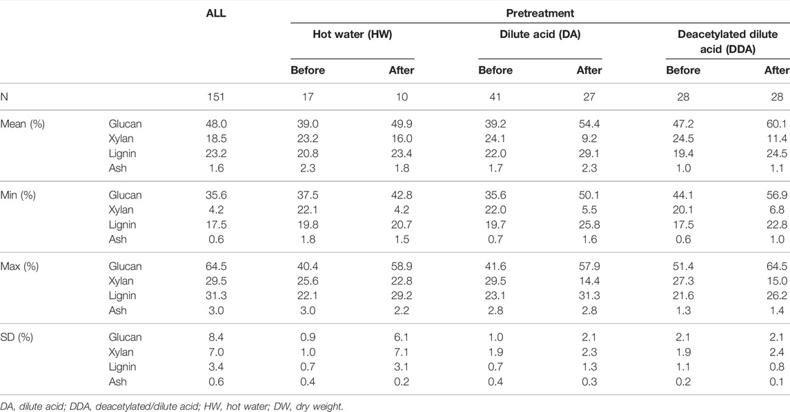
TABLE 1. Summary of compositional analysis data for population. Summary statistics for glucan, xylan, lignin and ash (%DW) content in the sample population used in this work. Summary statistics are shown for each of the pretreatments, with samples taken from catalyst-impregnated samples prior to (before) and after thermochemical pretreatment (after).

FIGURE 1

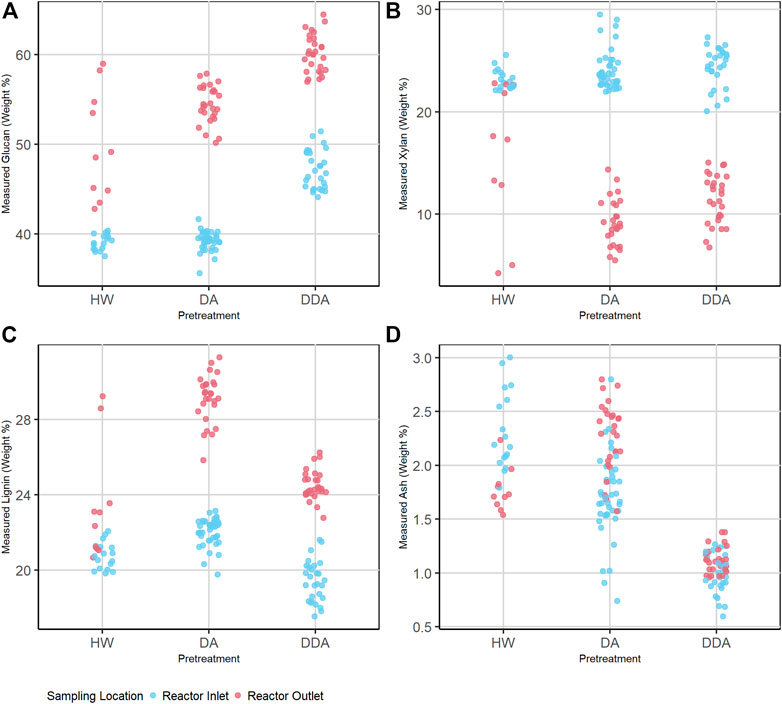
FIGURE 1. Dot plot depicting the distribution of primary analytical data (separated by pretreatment chemistry) of the combined calibration and independent validation sample set for glucan (A), xylan (B), lignin (C), and ash (D) content (%DW). Samples are prior to (before) and after thermochemical pretreatment (after), which is represented by color. Average measured glucan and lignin contents (%DW) increase and average measured xylan content (%DW) decreases after thermochemical pretreatment for all pretreatments. DDA treated samples show higher glucan and lower lignin and ash content than DA or HW. DA, dilute acid; DDA, deacetylated/dilute acid; Water, hot water; DW, dry weight.

3.1.1 Compositional Variability

The overall composition of the HW and DA samples taken at the reactor inlet are very similar for all four analytes, while the DDA samples taken at the reactor inlet are consistently higher in glucan content and lower in both lignin and ash content. The xylan content for inlet samples with all pretreatments is similar. Because the HW and DA samples from the reactor inlet had not yet been subject to elevated temperatures, and all samples were washed prior to analysis, these samples should be quite similar in glucan, xylan, and lignin content. The mean ash content of the DA samples is slightly lower than for the HW samples, since dilute acid is more aggressive in removing inorganic materials than water even at ambient temperature. The DDA samples at the reactor inlet had been subjected to deacetylation, which removes acetate side chains from hemicellulose, extractives, and a portion of lignin, xylan, and ash. Thus, this results in increased glucan content and reduced lignin and ash content. The loss in extractives, lignin, and ash, which collectively increases the remaining glucan content, is offset by the loss in hemicellulose during deacetylation, keeping the xylan content approximately constant.

Thermochemical pretreatment increases the glucan and lignin content and decreases the xylan content. Again, this is consistent with the chemistry of pretreatment, where elevated temperature and the presence of a catalyst (for DA and DDA) result in the solubilization of a large portion of the hemicellulose fraction, a small portion of the lignin fraction, but virtually none of the glucan fraction. This results in pretreated samples with substantially higher glucan, lower xylan, and higher lignin contents. The HW chemistry does not use a catalyst, and so is less effective in removing xylan and therefore enriching the sample in glucan and lignin. The larger variability in the post-pretreatment HW samples is due to the impact of reactor temperature and residence time—higher temperatures and longer residence times increase xylan removal and therefore increase the residual glucan and lignin contents (full data presented in Supplementary Material).

3.1.2 Spectral Variability

Figure 2 shows the mean values of the collected (A and B) and mathematically-transformed (C and D) NIR spectra both before (A and C) and after (column and D) thermochemical pretreatment for the three different pretreatments used in this work. As described previously, all collected spectra were mathematically transformed (normalization and derivatization) prior to use in model building.

FIGURE 2

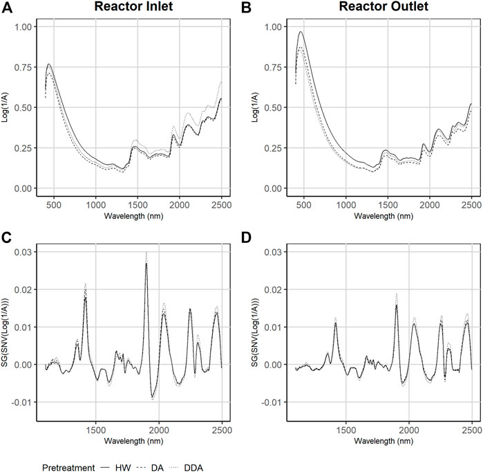
FIGURE 2. Average Near-infrared (NIR) and Visible (Vis) diffuse reflectance spectra collected across the three different pretreatments. Samples are taken from catalyst-impregnated samples prior to pretreatment (before) and after thermochemical pretreatment (after). Plots (A) and (B)—raw NIR spectra as collected. Plots (C) and (D)—NIR spectra after spectral transforming via Standard Normal Variate and Savitsky-Golay smoothing. DA, dilute acid; DDA, deacetylated/dilute acid; Water, hot water; DW, dry weight.

The collected spectra of samples taken before pretreatment (Figure 2A) have lower maximum absorbance at 500 nm in comparison to corresponding samples taken after pretreatment (Figure 2B) but have higher absorbance in the NIR range. The spectra of DDA samples show higher absorbance in the NIR range prior to pretreatment, while HW treated samples show the highest absorbance in the visible range after treatment. The transformed spectra of the samples collected prior to pretreatment are substantially different from the corresponding spectra collected after pretreatment. Close inspection of the transformed spectra shows that the HW and DA sample spectra are more similar to each other than to the DDA sample spectra, both before and after pretreatment. This is consistent with the differences in primary analytical chemistry—spectral variability follows compositional variability.

To investigate the spectral variability in more detail, we used Principal Component Analysis (PCA) to reduce the dimensionality of the transformed NIR spectra of the corn stover samples. Figure 3A shows a key result of this PCA in a score plot of the first two principal components. Sample points are colored by sampling location, and sample point symbols denote different pretreatment chemistries. The NIR spectra of the reactor inlet and reactor outlet samples are substantially different from each other (PC1), and the NIR spectra of the DDA samples are substantially different from the DA and HW samples (PC2). The DA and HW samples show substantial overlap. Note also that the NIR spectra of the independent validation samples held out of the model building (solid symbols) overlap the NIR spectra of the calibration samples (open symbols)—they are representative of the overall sample population and therefore a good indicator of model performance for spectra within the variance described by the calibration set. In Figure 3B we plot the glucan content vs. PC1 values. Glucan content correlates strongly and inversely with sampling location (r = −0.87)—samples taken from the reactor outlet have higher glucan content and lower PC1 values than reactor inlet samples. The separation of the population by chemistry seen in Figure 3A is still evident—DDA samples are consistently higher in glucan content than either HW or DA samples.

FIGURE 3

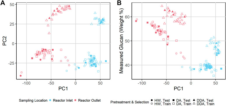
FIGURE 3. (A) Scatter plot of Principal Component 2 (PC 2) vs. PC 1 of transformed near-infrared (NIR) spectra of pretreated corn stover samples. The samples represent three different pretreatments. Samples are taken from catalyst-impregnated samples prior to (before) and after thermochemical pretreatment (after). The DA and HW samples appear more similar to each other than to the DDA samples. (B) Scatter plot of measured glucan content (%DW) vs. PC 1 of transformed NIR spectra of pretreated corn stover samples. PC 1 is highly correlated with the glucan content—variability in chemical composition strongly affects PC 1 variance, demonstrating that spectral variance follows composition variance. DDA samples have consistently higher glucan content than DA and HW samples (see text). DA, dilute acid; DDA, deacetylated/dilute acid; Water, hot water; DW, dry weight.

3.2 Construction of Quantitative Models

Supervised (PLS) and unsupervised (PCA) dimensionality reduction techniques were evaluated as additional spectral transformation techniques prior to SVM and RF. No additional spectral preprocessing was used for PLS. Dimensionality reduction using PLS resulted in better SVM models compared to either no dimensionality reduction or dimensionality reduction using PCA. No dimensionality reduction led to the best performing RF model. Details of these models are provided in the Supplementary Material—for the balance of this work we compare PLS, SVM with dimensionality reduction using PLS, and RF with no dimensionality reduction.

Figure 4A shows the variability in raw spectra observed in the biomass external reference check cells. Regions of high variability in check cell spectra occur at 1,400 and 1,900 nm, which correspond to the first overtone of the O-H stretch and the combination mode H-O-H bend and O-H stretch in water, respectively (Near-Infrared Spectroscopy in Agriculture, 2004). Ambient building sensor data showed fluctuations in both the relative humidity and temperature of the laboratory over that time. It is likely that these fluctuations are the root cause of this variability. Figure 4B compares the variability observed in the transformed check cell spectra to that observed in the training set. The variability observed at 1,900 nm in the check cells has a similar in range to that observed across the entire training set, suggesting that little useful compositional information can be obtained from this region of the spectra.

FIGURE 4

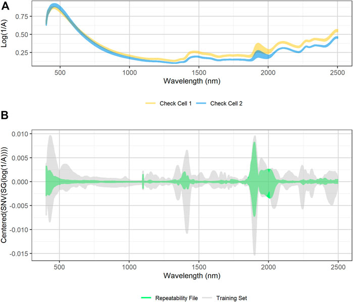
FIGURE 4. (A) Plot of raw diffuse reflectance spectra of external standard materials check cells. The two external standard material check cells were created at the beginning of the project from two unique pretreated corn stover feedstocks. The check cells were scanned 15 times over the course of 6 months. High variability in the reflectance spectra exists at 1,900 nm, which corresponds to a known water overtone (B) SNV/SG/centered spectra of calibration spectra (grey) overlaid with SNV/SG/centered difference spectra of the external standard material check cells (green). The variability of the calibration spectral between 1,900 and 2,050 nm is similar in magnitude to the variability observed in the external standard material check cells. The ratio of calibration spectra variability to repeatability file variability is low in the visible region below 500 nm, at the 1,100 nm detector change, and at 1,400 nm, which corresponds to another water peak.

Figure 5 compares the performance results (measured as RMSE) for cross validation (Figures 5A–D), independent validation Figures 5E–H, and late training validation (Figures 5I–L) for PLS, RF, and SVM models made with and without the addition of the check cell spectra variability to the calibration set through implementation of the “repeatability file” strategy. The tabulated results are presented in the Supplementary Material. SVM and PLS models showed statistically significant improvements in glucan, xylan, and ash performance across the independent validation and late training sets with the inclusion of a repeatability file (α = 0.05). These results support the idea that the repeatability file improves NIR model performance for outcomes that are highly influenced by water when PLS is used for dimensionality reduction. All models predicting lignin showed no statistically significant improvement with the addition of a repeatability file, indicating that the prediction of lignin from pretreated biomass via NIR is more robust to the environmental variability encountered during this work than the structural carbohydrates.

FIGURE 5

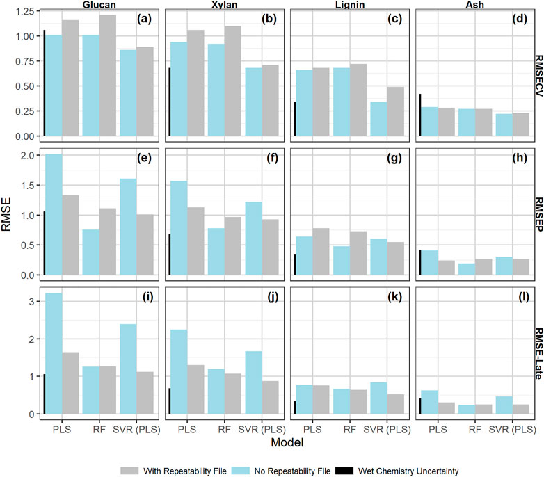
FIGURE 5. Bar chart of the model performance measured by RMSE values by constituent with the calibration data set alone or augmented by the check cell difference spectra, the “repeatability file” strategy. The measures of performance shown are as follows: (A–D) : RMSECV (root mean square error of 10 × 10-fold cross validation); (E–H): the RMSEP root mean square error of prediction; (I–L): the RMSE-late (root mean square error of late scan predictions). The measurement uncertainty associated with the primary analytical method, (Templeton et al., 2010) which is two times the standard deviation from the primary analytical method, is shown for scale as the leftmost black bar on each graph. The “repeatability file” algorithm improves the performance of the SVM and PLS models as measured by RMSEP and RMSE-late but has little effect on the RF model (see text).

RF models showed no significant difference in performance with the use of the “repeatability file” strategy. Random forest models are known to be robust against the inclusion of unimportant predictors and outliers (Breiman, 2001; Lee et al., 2013). Because of the algorithm’s robustness against unimportant variables, inclusion of the NIR regions with high check cell variability had no substantial impact on the model performance, regardless of whether a repeatability file is added. Furthermore, the decision tree algorithm used in RF models treats the repeatability file check cell variance like outliers to the calibration set rather than variance to ignore. The nonlinear nature of the individual decision trees is robust against such outliers, making the addition of the check cell spectra in the repeatability file algorithm superfluous—it neither improves the model by decreasing the effect of this variability nor decreases model performance by including this variability. A comparison of the variable importance predictor scores between the RF models with and without the inclusion of the repeatability file (Supplementary Material) shows little change in which predictors are used in modeling.

3.3 Modeling Algorithm Comparisons

In Table 2 we show the R² and RMSE values for all four analytes of interest (glucan, xylan, lignin, ash) for all three modeling approaches (PLS, SVM, RF) for calibration, cross-validation, independent validation, and late training. For these models, the calibration data set was augmented with repeated check cell spectra using the “repeatability file” strategy.

TABLE 2

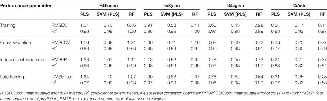
TABLE 2. Summary of model performance results by constituent. Performance results for each model build for each constituent of interest.

The SVM algorithm resulted in the statistically significantly better cross validation performance compared to both PLS and RF across all constituents. The best SVM models had an RMSECV of 0.89 for glucan content, 0.71 for xylan content, 0.49 for lignin content, and 0.23 for ash content. No statistically significant differences were found between the RF and PLS model RMSECV results for any analyte.

Prediction performance with an independent validation set is a more stringent test of model performance than cross-validation. The performance results for the independent validation predictions (RMSEP) were mixed between the different model types. The SVM algorithm predicted glucan, xylan, and lignin content from the independent validation set with greater accuracy than the PLS algorithm. The residual plots included in the Supplementary Material graphically demonstrate the reduced scatter in the prediction residuals and reduced bias in samples with high glucan content with the SVM algorithm. The RF algorithm predicted glucan and xylan content with greater accuracy than the PLS algorithm, while the SVM algorithm resulted in better accuracy at predicting lignin content and reduced bias in samples with high glucan content than RF, but similar overall performance at predicting xylan content. All modeling techniques resulted in similar prediction performance at predicting ash content for the independent validation set.

Finally, the prediction performance of the rescanned calibration set (the “late-training” set described above) is another test of model performance which includes the model’s ability to differentiate instrumental or environmental variance from variance associated with wet chemistry. The SVM algorithm showed better performance at predicting all constituents using the late training set as compared to PLS, and better performance at predicting xylan and lignin content than RF. SVM and RF had similar performance for predicting ash and glucan content. RF models predicted all constituents with higher accuracy than PLS.

While all three algorithms provided acceptable models, the RF algorithm required more computational resources—approximately 10–20 times longer than either the PLS or SVM algorithms. Final versions of the RF models were trained using a local HPC cluster, while the final PLS and SVM models were trained on a standard laptop computer.

Figures 6, 7 show the predicted versus measured cross validation and independent validation results across the three modeling techniques for measured glucan and lignin content (%DW). Similar plots for measured xylan and ash, as well as residual plots for all four constituents, are provided in the Supplementary Material. In agreement with the statistics presented in Table 2 and discussed above, graphical displays of model performance show all three algorithms provide acceptable prediction results for all constituents, with the SVM modeling results appearing slightly superior to PLS and RF for both the cross-validation and independent validation predictions. In particular, we observe that the SVM modeling algorithm appears to provide better glucan predictions for the samples with the highest glucan content (as measured by prediction residuals).

FIGURE 6

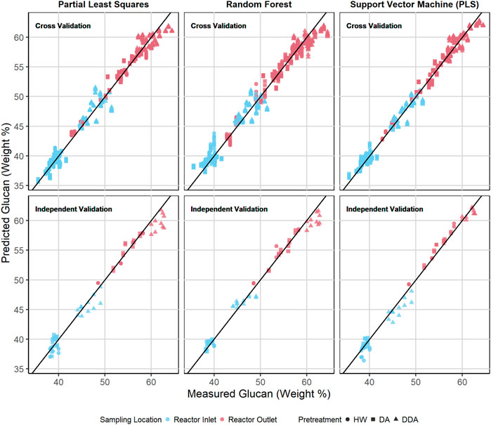
FIGURE 6. Predicted vs. measured glucan content (%DW) for PLS, RF, and SVM models. The symbol shape represents the different pretreatment used, while the color represents the sampling location—before or after thermochemical pretreatment. The upper row depicts the repeated 10-fold cross validation results for each model. The lower row depicts the independent validation results for each model. DA, dilute acid; DDA, deacetylated/dilute acid; Water, hot water; DW, dry weight.

FIGURE 7

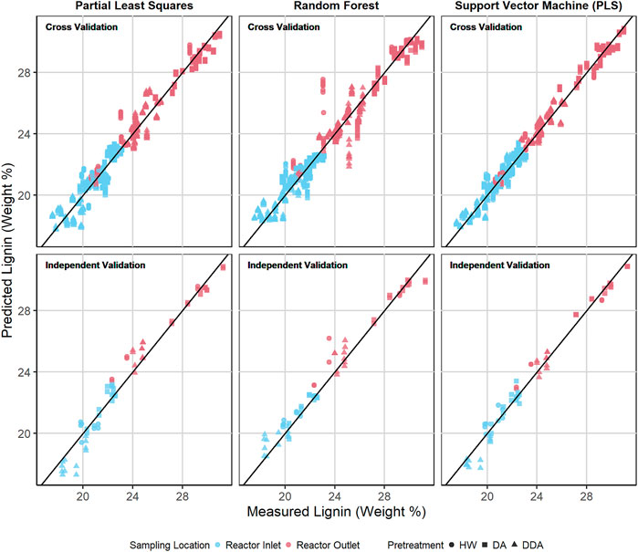
FIGURE 7. Predicted vs. measured lignin content (%DW) for PLS, RF, and SVM models. The symbol shape represents the different pretreatment used, while the color represents the sampling location—before or after thermochemical pretreatment. The upper row depicts the repeated 10-fold cross validation results for each model. The lower row depicts the independent validation results for each model.

Moreover, a single model can accurately predict the composition of corn stover samples undergoing three different pretreatment chemistries (HW, DA, DDA) and at multiple locations within the process (before and after the thermochemical pretreatment reactor). We believe this has substantial implications on the feasibility of real-time characterization using on-line NIR spectroscopy—a single model could be built and maintained for implementation at multiple points in the process.

Discussions about the relative performance of different modeling approaches or different modeling algorithms should take the uncertainty of the primary analytical data used as the dependent variables into account. Differences in RMSE values smaller than the primary analytical uncertainties are not practically significant. In Figure 5 we include a small vertical bar in all plots corresponding to the uncertainty of the primary analytical chemistry (Templeton et al., 2010) estimated as two times the standard deviation of multiple replicate measurements by analysts. Thus, the improvements in both glucan and xylan RMSE-late values for the PLS and SVM models by using the “repeatability file” strategy are both statistically and practically significant, while the improvements in the ash predictions for these models are statistically significant but not practically significant.

RMSE values like those presented for the PLS, SVM, and RF models developed in this work provide an estimate of the average uncertainty for samples in the model population (e.g., training, independent validation). However, they do not provide an estimate of uncertainty of a specific prediction. Like in primary analytical chemistry measurements, some estimation of the uncertainty of a specific prediction from a rapid characterization model is important to provide a quantitative estimate of the confidence the user should have in that specific prediction.

Linear modelling approaches like PLS have a robust literature discussing this issue (Faber, 2005; Olivieri et al., 2006; Zhang and Garcia-Munoz, 2009; Garrido-Varo et al., 2019; Emil Eskildsen and Næs, 2020). Some measures of uncertainty calculate a confidence interval for the prediction similarly to that of a linear model where the confidence interval increases with the distance in multivariate space from the spectra to be predicted to the center of the calibration population and decreases as the quality of the calibration model increases. Other uncertainty measures calculate a population membership region based on the Mahalanobis distance of a sample to the center of the calibration population. This is the basis of the well-known global-H, neighborhood-H (GH, NH) statistic (Westerhaus, 2014).

While a detailed comparison of these different uncertainty measures is beyond the scope of this work, we wish to point out that these measures are based on an evaluation of spectral similarity in a linear modeling framework (e.g., PLS, PCA, PCR). Thus, such uncertainty estimates may be appropriate for use with Support Vector Regression even with nonlinear kernels if a linear dimensionality reduction technique (like PCA or PLS) is used. However, Random Forest Regression is a nonlinear technique, and use of uncertainty estimations using such assumptions are inappropriate. There has been some research into uncertainty measures for RF (McAlexander and Mentch, 2020; Tavazza et al., 2021), but consensus on the best approach has not been reached, nor has the application of any specific approach to RF models based on spectroscopy been demonstrated. In the absence of such consensus, a concern with using an RF model is the inability to estimate a confidence interval for individual predictions.

3.4 Selecting a Model

In this work we have compared the performance of three different modelling approaches (PLS, SVM, and RF) for developing a rapid characterization model for a population of pretreated corn stover samples using three different pretreatment chemistries. All three approaches resulted in acceptable models as measured by multiple RMSE assessments (training, cross-validation, independent validation, late-training) when compared to the uncertainty in the primary analytical chemistry methods. The use of repeated check cell spectra via the “repeatability file” strategy improved the performance of both the PLS and SVM algorithms. The RF algorithm performed equivalently with or without a “repeatability file”. The use of dimensionality reduction via PLS improved the performance of the SVM algorithm. The RF algorithm performed best without any dimensionality reduction. While all three algorithms provided acceptable models, the RF algorithm required more computational resources—RF models took approximately 10–20 times longer to solve than the either PLS or SVM models. Multiple robust estimations of prediction uncertainty exist for the PLS algorithm, and these uncertainty algorithms can also be used for SVM algorithms when dimensionality reduction is used as an additional spectral preprocessing step. No such robust estimates of uncertainty exist for the RF algorithm.

Based on these results, we believe the SVM algorithm is the method of choice for this dataset when used with both the “repeatability file” strategy and dimensionality reduction using PLS. The SVM algorithm presents a good compromise between computational efficiency and prediction performance and permits the use of multiple robust estimations of individual prediction uncertainties.

Data Availability Statement

The raw data supporting the conclusion of this article will be made available by the authors, without undue reservation.

Author Contributions

EW conceived of the study and supervised its execution. ZT contributed to the model selection, performed all spectral acquisition, data organization and reduction, all modelling, statistical analysis of modelling results, and prepared all figures and tables. ZT and EW jointly drafted and edited the manuscript.

Funding

This work was funded by the National Renewable Energy Laboratory, operated by Alliance for Sustainable Energy, LLC, for the U.S. Department of Energy (DOE) under Contract No. DE-AC36-08GO28308. Funding provided by the U.S. Department of Energy Office of Energy Efficiency and Renewable Energy Bioenergy Technologies Office. The views expressed in the article do not necessarily represent the views of the DOE or the U.S. Government.

Author Disclaimer

The views expressed in the article do not necessarily represent the views of the DOE or the U.S. Government. The U.S. Government retains and the publisher, by accepting the article for publication, acknowledges that the U.S. Government retains a nonexclusive, paid-up, irrevocable, worldwide license to publish or reproduce the published form of this work, or allow others to do so, for U.S. Government purposes.

Conflict of Interest

The authors declare that the research was conducted in the absence of any commercial or financial relationships that could be construed as a potential conflict of interest.

Publisher’s Note

All claims expressed in this article are solely those of the authors and do not necessarily represent those of their affiliated organizations, or those of the publisher, the editors and the reviewers. Any product that may be evaluated in this article, or claim that may be made by its manufacturer, is not guaranteed or endorsed by the publisher.

Acknowledgments

The experimental data used in this work were generated at the NREL Integrated Biorefinery Research Facility (IBRF) under a Cooperative Research and Development Agreement (CRADA) funded by ExxonMobil. The authors acknowledge the reviewers for helpful suggestions to improve the manuscript.

Supplementary Material

The Supplementary Material for this article can be found online at: https://www.frontiersin.org/articles/10.3389/fenrg.2022.878973/full#supplementary-material

References

Abrams, S. M., Shenk, J. S., Westerhaus, M. O., Barton, F. E., and Barton, F. E. (1987). Determination of Forage Quality by Near Infrared Reflectance Spectroscopy: Efficacy of Broad-Based Calibration Equations. J. Dairy Sci. 70, 806–813. Available at: http://jds.fass.org/cgi/content/abstract/70/4/806. doi:10.3168/jds.s0022-0302(87)80077-2

CrossRef Full Text | Google Scholar

Acharya, U. K., Walsh, K. B., and Subedi, P. P. (2014). Robustness of Partial Least-Squares Models to Change in Sample Temperature: I. A Comparison of Methods for Sucrose in Aqueous Solution. J. Near Infrared Spectrosc. 22, 279–286. doi:10.1255/jnirs.1113

CrossRef Full Text | Google Scholar

Awad, M., and Khanna, R. (2015). “Support Vector Regression,” in Efficient Learning Machines: Theories, Concepts, and Applications for Engineers and System Designers. Editors M. Awad, and R. Khanna (Berkeley, CA: Apress), 67–80. doi:10.1007/978-1-4302-5990-9_4

CrossRef Full Text | Google Scholar

Beebe, K. R., Pell, R. J., and Seasholtz, M. B. (1998). Chemometrics: A Practical Guide. New York: Wiley and Sons.

Google Scholar

Breiman, L. (2001). Random Forests. Mach. Learn. 45, 5–32. doi:10.1023/A:1010933404324

CrossRef Full Text | Google Scholar

Chanda, S., Hazarika, A. K., Choudhury, N., Islam, S. A., Manna, R., Sabhapondit, S., et al. (2019). Support Vector Machine Regression on Selected Wavelength Regions for Quantitative Analysis of Caffeine in Tea Leaves by Near Infrared Spectroscopy. J. Chemom. 33, e3172. doi:10.1002/cem.3172

CrossRef Full Text | Google Scholar

Cristianini, N., and Shawe-Taylor, J. (2000). An Introduction to Support Vector Machines and Other Kernel-Based Learning Methods. Cambridge: Cambridge University Press. doi:10.1017/CBO9780511801389

CrossRef Full Text | Google Scholar

de Santana, F. B., de Souza, A. M., and Poppi, R. J. (2018). Visible and Near Infrared Spectroscopy Coupled to Random Forest to Quantify Some Soil Quality Parameters. Spectrochimica Acta Part A Mol. Biomol. Spectrosc. 191, 454–462. doi:10.1016/j.saa.2017.10.052

CrossRef Full Text | Google Scholar

de Santana, F. B., Otani, S. K., de Souza, A. M., and Poppi, R. J. (2021). Comparison of PLS and SVM Models for Soil Organic Matter and Particle Size Using Vis-NIR Spectral Libraries. Geoderma Reg. 27, e00436. doi:10.1016/j.geodrs.2021.e00436

CrossRef Full Text | Google Scholar

Emil Eskildsen, C., and Næs, T. (2020). Sample-Specific Prediction Error Measures in Spectroscopy. Appl. Spectrosc. 74, 791–798. doi:10.1177/0003702820913562

PubMed Abstract | CrossRef Full Text | Google Scholar

Faber, K. (2005). Multivariate Prediction Uncertainty. Available at: www.chemometrics.com (Accessed February 2, 2022).

Google Scholar

Fawagreh, K., Gaber, M. M., and Elyan, E. (2014). Random Forests: From Early Developments to Recent Advancements. Syst. Sci. Control Eng. 2, 602–609. doi:10.1080/21642583.2014.956265

CrossRef Full Text | Google Scholar

Garrido-Varo, A., Garcia-Olmo, J., and Fearn, T. (2019). A Note on Mahalanobis and Related Distance Measures in WinISI and the Unscrambler. J. Near Infrared Spectrosc. 27, 253–258. doi:10.1177/0967033519848296

CrossRef Full Text | Google Scholar

Geladi, P., and Kowalski, B. R. (1986). Partial Least-Squares Regression: A Tutorial. Anal. Chim. Acta 185, 1–17. doi:10.1016/0003-2670(86)80028-9

CrossRef Full Text | Google Scholar

Höskuldsson, A. (1988). PLS Regression Methods. J. Chemom. 2, 211–228. doi:10.1002/cem.1180020306

CrossRef Full Text | Google Scholar

Kelley, S. S., Jellison, J., and Goodell, B. (2002). Use of NIR and Pyrolysis-MBMS Coupled with Multivariate Analysis for Detecting the Chemical Changes Associated with Brown-Rot Biodegradation of Spruce Wood. FEMS Microbiol. Lett. 209 (02), 107–111. doi:10.1111/j.1574-6968.2002.tb11117.x

PubMed Abstract | CrossRef Full Text | Google Scholar

Labbé, N., Lee, S.-H., Cho, H.-W., Jeong, M. K., and André, N. (2008). Enhanced Discrimination and Calibration of Biomass NIR Spectral Data Using Non-Linear Kernel Methods. Bioresour. Technol. 99, 8445–8452. doi:10.1016/j.biortech.2008.02.052

PubMed Abstract | CrossRef Full Text | Google Scholar

Lee, S., Choi, H., Cha, K., and Chung, H. (2013). Random Forest as a Potential Multivariate Method for Near-Infrared (NIR) Spectroscopic Analysis of Complex Mixture Samples: Gasoline and Naphtha. Microchem. J. 110, 739–748. doi:10.1016/j.microc.2013.08.007

CrossRef Full Text | Google Scholar

McAlexander, R. J., and Mentch, L. (2020). Predictive Inference with Random Forests: A New Perspective on Classical Analyses. Res. Polit. 7, 205316802090548. doi:10.1177/2053168020905487

CrossRef Full Text | Google Scholar

Near‐Infrared Spectroscopy in Agriculture (2004). Near‐Infrared Spectroscopy in Agriculture. 1st ed. Madison, WI: John Wiley & Sons. doi:10.2134/agronmonogr44

CrossRef Full Text | Google Scholar

Olivieri, A. C., Faber, N. M., Ferré, J., Boqué, R., Kalivas, J. H., and Mark, H. (2006). Uncertainty Estimation and Figures of Merit for Multivariate Calibration (IUPAC Technical Report). Pure Appl. Chem. 78, 633–661. doi:10.1351/pac200678030633

CrossRef Full Text | Google Scholar

Pasquini, C. (2018). Near Infrared Spectroscopy: A Mature Analytical Technique with New Perspectives - A Review. Anal. Chim. Acta 1026, 8–36. doi:10.1016/j.aca.2018.04.004

PubMed Abstract | CrossRef Full Text | Google Scholar

Roggo, Y., Duponchel, L., Ruckebusch, C., and Huvenne, J.-P. (2003). Statistical Tests for Comparison of Quantitative and Qualitative Models Developed with Near Infrared Spectral Data. J. Mol. Struct. 654, 253–262. doi:10.1016/S0022-2860(03)00248-5

CrossRef Full Text | Google Scholar

Sanderson, M. A., Agblevor, F., Collins, M., and Johnson, D. K. (1996). Compositional Analysis of Biomass Feedstocks by Near Infrared Reflectance Spectroscopy. Biomass Bioenergy 11, 365–370. doi:10.1016/S0961-9534(96)00039-6

CrossRef Full Text | Google Scholar

Shekiro, J., Kuhn, E. M., Nagle, N. J., Tucker, M. P., Elander, R. T., and Schell, D. J. (2014). Characterization of Pilot-Scale Dilute Acid Pretreatment Performance Using Deacetylated Corn Stover. Biotechnol. Biofuels 7, 23. doi:10.1186/1754-6834-7-23

PubMed Abstract | CrossRef Full Text | Google Scholar

Shenk, J. S., and Westerhaus, M. O. (1991). New Standardization and Calibration Procedures for Nirs Analytical Systems. Crop Sci. 31, 1694–1696. doi:10.2135/cropsci1991.0011183X003100060064x

CrossRef Full Text | Google Scholar

Skvaril, J., Kyprianidis, K. G., and Dahlquist, E. (2017). Applications of Near-Infrared Spectroscopy (NIRS) in Biomass Energy Conversion Processes: A Review. Appl. Spectrosc. Rev. 52, 675–728. doi:10.1080/05704928.2017.1289471

CrossRef Full Text | Google Scholar

Tavazza, F., DeCost, B., and Choudhary, K. (2021). Uncertainty Prediction for Machine Learning Models of Material Properties. ACS Omega 6, 32431–32440. doi:10.1021/acsomega.1c03752

PubMed Abstract | CrossRef Full Text | Google Scholar

Templeton, D. W., Scarlata, C. J., Sluiter, J. B., and Wolfrum, E. J. (2010). Compositional Analysis of Lignocellulosic Feedstocks. 2. Method Uncertainties. J. Agric. Food Chem. 58, 9054–9062. doi:10.1021/jf100807b

PubMed Abstract | CrossRef Full Text | Google Scholar

Tsuchikawa, S. (2007). A Review of Recent Near Infrared Research for Wood and Paper. Appl. Spectrosc. Rev. 42, 43–71. doi:10.1080/05704920601036707

CrossRef Full Text | Google Scholar

Tsuchikawa, S., and Kobori, H. (2015). A Review of Recent Application of Near Infrared Spectroscopy to Wood Science and Technology. J. Wood Sci. 61, 213–220. doi:10.1007/s10086-015-1467-x

CrossRef Full Text | Google Scholar

Westerhaus, M. (2014). Eastern Analytical Symposium Award for Outstanding Achievements in Near Infrared Spectroscopy: My Contributions to Near Infrared Spectroscopy. NIR News 25, 16–20. doi:10.1255/nirn.1492

CrossRef Full Text | Google Scholar

Xiao, L., Wei, H., Himmel, M. E., Jameel, H., and Kelley, S. S. (2014). NIR and Py-Mbms Coupled with Multivariate Data Analysis as a High-Throughput Biomass Characterization Technique: A Review. Front. Plant Sci. 5, 388. doi:10.3389/fpls.2014.00388

PubMed Abstract | CrossRef Full Text | Google Scholar

Zhang, L., and Garcia-Munoz, S. (2009). A Comparison of Different Methods to Estimate Prediction Uncertainty Using Partial Least Squares (PLS): A Practitioner’s Perspective. Chemom. Intell. Lab. Syst. 97, 152–158. doi:10.1016/j.chemolab.2009.03.007

CrossRef Full Text | Google Scholar