Modeling Soil-Facing Interface Interaction With Continuum Element Methodology

Introduction

Soil-facing mechanical interactions play an important role in the behavior of earth-retaining walls. Generally, numerical analysis of earth-retaining structures requires the use of interface elements between dissimilar component materials to model soil–structure interactions and to capture the transfer of normal and shear stresses through these discontinuities (Carter et al., 2000; Ng et al., 1997; Desai et al., 1984). Although this article is motivated by geotechnical modeling of earth-retaining structures, interface elements are required for a range of geotechnical and geoenvironmental model problems.

In finite element method (FEM) software programs, soil–structure interactions can be modeled using special interface “zero-thickness” interface elements between the soil and structural components (Day and Potts, 1994; Goodman et al., 1968). These elements use a strength/stiffness reduction factor that is applied to the soil adjacent to the interface.

Some software programs do not have a specific tool to model interfaces; thus, continuum elements are necessary to model soil–structure, soil–reinforcement interactions, and other interaction problems. The continuum element approach has the advantage of more control of the interface features (i.e., constitutive material strength and stiffness properties), as well as the element sizes and shapes at the interfaces. A methodology and proposed parameter values for continuum elements using CODE_BRIGHT software (Olivella et al., 1996) are presented in the following sections that give the same numerical outcomes as those using zero-thickness elements in already calibrated/validated two-dimensional (2D) models.

In earth-retaining walls, soil-facing interaction may not require specific 3D modeling because general 2D plane strain modeling has been demonstrated to give good performance. This is particularly true for reinforced soil wall problems (related/representative examples including 2D soil-facing interface treatments in calibrated reinforced soil wall modeling are those of Huang et al., 2009, Damians I. P. et al., 2015; Yu and Bathurst 2017). However, in some cases, the use of continuum elements can give unexpected results when using elastic–plastic soil models, such as stress fluctuations once soil plastic flow occurred (Damians I. P. et al., 2015). Moreover, because soil-facing interaction is also required in 3D analyses (e.g., the inside surface of the facing in reinforced soil wall modeling cases, see Damians et al., 2021; Won and Lancuyan 2020; Montilla et al., 2022), 3D soil-facing interfaces should be used, subject to careful calibration and validation.

The main objectives of this study are, first, to examine the load transfer between the soil and the facing component within a small concrete earth-retaining wall segment using both zero-thickness (PLAXIS, 2008; PLAXIS, 2012) and spring elements (FLAC, Itasca, 2011), and continuum elements at the interfaces using these finite element and finite difference model programs; second, to present numerical model details for equivalent interface property values using the different default interface modeling methods available or the proposed methodology with continuum elements; and third, to apply the same continuum modeling approach to simple 3D model cases with CODE_BRIGHT and to compare outcomes using the matching 2D plane strain approach.

General Problem Definition

A small concrete earth-retaining structure segment was considered to examine the load transfer from the backfill soil to the adjacent facing structure using both zero-thickness elements and continuum elements with the same interface property values (Figure 1). The concrete facing was 0.5 m thick and 1.5 m high. The retained backfill soil was 2.5 m long and 1.5 m high. Both the soil and concrete facing were discretized using 15-node elements. The left side of the concrete facing and the right side of the backfill soil were fixed in x-direction and free in y-direction. The bottom of both the concrete facing and backfill soil was fixed in y-direction only. A uniformly distributed surcharge load with three different magnitudes (q = 10, 50, and 100 kPa) was applied to the top surface of the backfill soil.

FIGURE 1

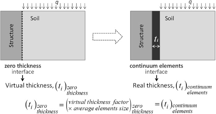
FIGURE 1. Interface modeling approaches with zero-thickness elements and continuum elements (Damians et al. 2015b).

The soil was modeled as linear elastic with Mohr–Coulomb failure criterion. The parameter values for the backfill soil are shown in Table 1. The concrete facing was modeled as linear elastic with elastic modulus of 32 GPa, Poisson ratio of 0.15, and a unit weight of 25 kN/m³. The interface strength and stiffness can be very different, depending on the interacting materials (Potyondy 1961). Thus, five different strength/stiffness reduction factors (R_i = 0.3, 0.45, 0.6, 0.8, and 1.0) were considered; the corresponding interface property values are shown in Supplementary Table S1 (Supplemental Material).

TABLE 1

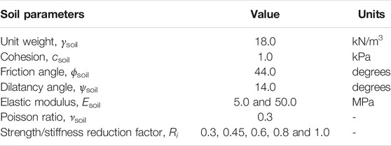
TABLE 1. Soil properties.

As an elastic–plastic model with the Mohr–Coulomb failure criterion, the proposed continuum element interfaces have strength properties of friction angle (ϕ_i), cohesion (c_i), and dilatancy angle (assumed with a fixed value of ψ_i = 0°). The stiffness of the interface is controlled by Young modulus (E_i) and the Poisson ratio (assumed with a fixed value of v_i = 0.45).

The parameter relations between the soil and the interface material can be understood as a strength/stiffness reduction factor (R_i ≤ 1.0) directly applied to the properties of the adjacent soil. Thus, to set the interface material properties, the following parameter relationships are considered:

$c_i=R_i{c}_{soil}(1)$

${\varphi }_i={\tan }^{-1}\left(R_i\tan {\varphi }_{soil}\right)(2)$

$G_i=R_i^2{G}_{soil}=R_i^2\left(\frac{E_{soil}}{2\left(1+{\nu }_{soil}\right)}\right)(3)$

$E_{\text{oed,i}}=2G_{\text{i}}\frac{1-v_{\text{i}}}{1-2v_{\text{i}}}(4)$

where c_soil is the _soil cohesion; ϕ_soil is the soil friction angle; E_soil is the Young modulus of the soil; G_soil and G_i are the shear modulus of the soil and the interface, respectively, and E_oed,i corresponds to the oedometer modulus of the interface material (because, as mentioned, v_i = 0.45).

From Eq. 4, Young modulus of the interface can be deduced as follows:

$E_i=2G_i\left(1+{\nu }_i\right)=R_i^2\left(\frac{E_{soil}}{(1+{\nu }_{soil})}\right)\left(1+{\nu }_i\right)=1.45R_i^2\left(\frac{E_{soil}}{(1+{\nu }_{soil})}\right)(5)$

First, a 2D approach is used to examine the influence of the mesh size on the analysis of soil-facing interaction.

2D Modeling

Interface 2D Model and Properties With PLAXIS

To model an interface with continuum elements, a real interface zone between the dissimilar materials with the thickness equal to the virtual thickness from the zero-thickness elements is generated (Figure 1). The material properties of this zone are also taken to be the same as those from the zero-thickness elements. For cases where different finite element meshes (with different average element sizes) are considered, the virtual thickness factor can be slightly adjusted to keep the same interface virtual thickness. Unless otherwise specified, the actual thickness value considered was 18 mm, corresponding to the exact value used during calculation. This value can be found in the output (a postprocessor in PLAXIS), but requires checking and possible adjustment using iterative cycles of updated input meshing, examining the output file and rerunning the program.

Effect of the Mesh Size and Element Type

Figure 2 shows three different finite element meshes (i.e., coarse, fine, and optimized) that were generated to examine the effect of element size at the interface zone on the load transfer between the soil and facing structure. The coarse mesh (Figure 2A) had the highest element aspect ratio within the real interface zone; the optimized mesh (Figure 2C) had the lowest element aspect ratio in the region where the analysis is focused (and fewer total number of elements), and the element aspect ratio of the fine mesh (Figure 2B) was between that of the coarse and optimized meshes. When zero-thickness elements were used at the interface between the soil and facing, the interface virtual thickness was 18 mm as mentioned earlier. When using continuum elements to simulate the soil-facing interaction, the same 18 mm-value of real zone thickness was modeled (see Figure 2—Details).

FIGURE 2

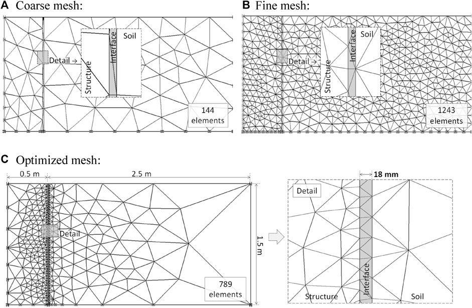
FIGURE 2. Three different finite element meshes (15 node triangular elements) for the same soil–structure interaction example using program PLAXIS: (A) coarse mesh, (B) fine mesh, and (C) optimized mesh with the same interface thickness of ti = 0.018 m (Damians et al. 2015b).

Figure 3 shows the normal and shear stresses acting at the interface between the facing and backfill soil with the three different meshes and using the strength/stiffness reduction factor of R_i = 0.8 where both zero-thickness elements and continuum elements are considered. The use of R_i = 0.8 results in an interface friction angle of approximately 38°, which is similar to the measured friction angle between smooth concrete and sand (Potyondy 1961; Samtani and Nowatzki 2006). The numerical modeling showed that for the cases examined with zero-thickness elements, the finite element mesh had a minor effect on the normal and shear stresses at the interface between the soil and facing. However, when using continuum elements, both interface normal and shear stresses fluctuated once soil plastic flow occurred for all three meshes. The results also showed that the optimized mesh with the lowest interface continuum element aspect ratio experienced the smallest stress fluctuation amplitudes.

FIGURE 3

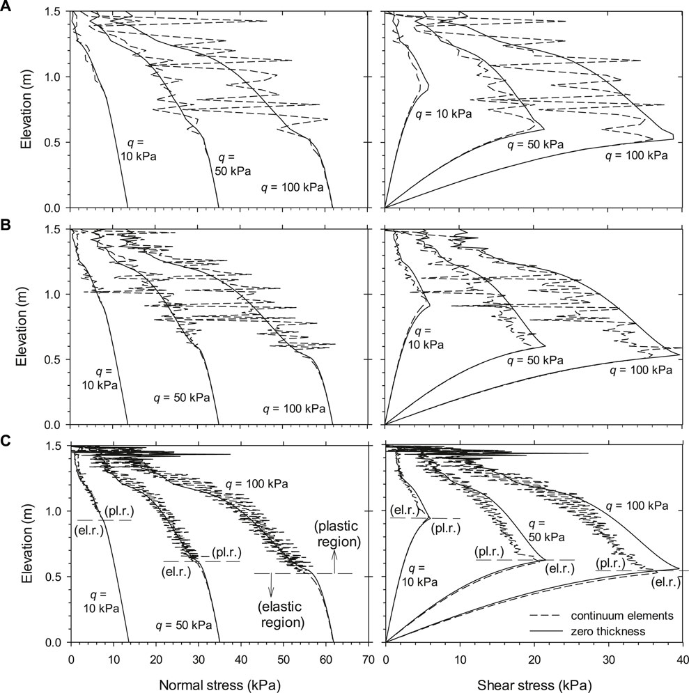
FIGURE 3. Load transfer from backfill soil to facing panel using PLAXIS: effect of the finite element mesh on the normal and shear stresses at the interface between the facing structure and backfill soil: (A) coarse mesh, (B) fine mesh, and (C) optimized mesh. Cases with Ri = 0.8 (Damians et al. 2015b).

The total horizontal and vertical forces acting at the interface are shown in Supplementary Tables S2, S3, respectively. Both total horizontal and vertical forces using zero-thickness elements are in good agreement with results using continuum elements, and the finite element mesh had a minor effect on the total horizontal and vertical forces for both zero-thickness elements and continuum elements.

Effect of the Strength/Stiffness Reduction Factor

Figure 4 shows the normal and shear stresses at the interface between the facing structure and backfill soil for the three different strength/stiffness reduction factors investigated. The modeling results showed that for the continuum elements, increasing the strength/stiffness reduction factor (i.e., increasing the interface stiffness) resulted in greater amplitude of both normal and shear stress fluctuations in the plastic region when other conditions were equal. However, as presented in Supplementary Table S3 in the Supplemental Material, the total vertical loads (i.e., equivalent force from shear stresses) at the interface between the facing and backfill soil from the continuum elements are in good agreement with those from simulations with zero-thickness elements.

FIGURE 4

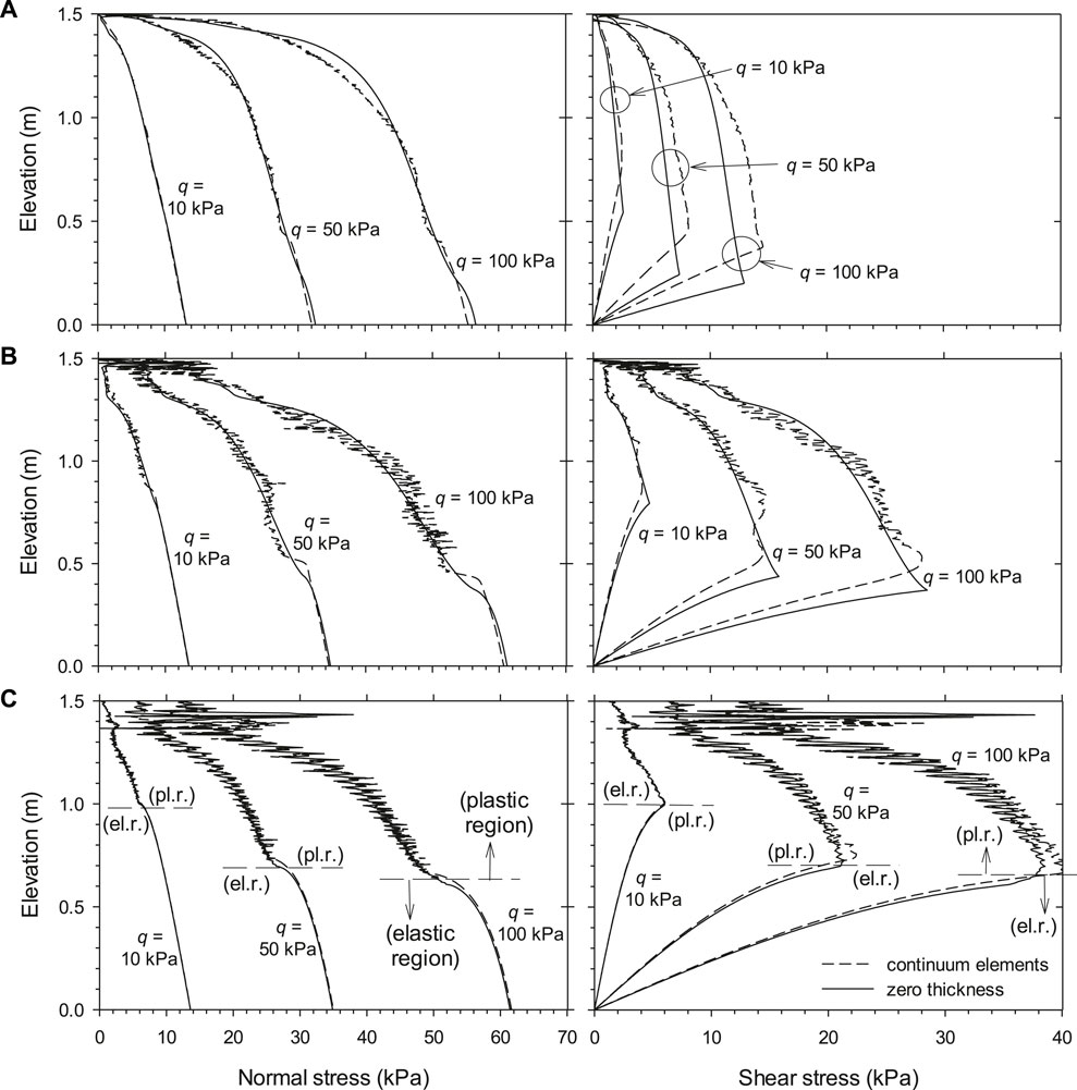
FIGURE 4. Load transfer from backfill soil to facing panel using PLAXIS: normal and shear stresses at the interface between facing structure and backfill soil with optimized mesh for three different strength/stiffness reduction factors: (A) Ri = 0.3, (B) Ri = 0.6, and (C) Ri = 1.0 (Damians et al. 2015b).

Equivalent Interface Properties Between FLAC and PLAXIS

The interface friction angle, cohesion, dilatancy angle, and tensile strength in FLAC are the same as those in PLAXIS, and the same parameter values can be set directly in both programs. If the normal stiffness (k_n) and shear stiffness (k_s) from FLAC are known, the equivalent interface properties in PLAXIS can be found using the following equations (Yu et al., 2014 and 2015):

$E_{\text{i}}=\frac{\left(3k_{\text{n}}-4k_{\text{s}}\right)k_{\text{s}}{t}_{\text{i}}}{k_{\text{n}}-k_{\text{s}}}(6)$

$v_{\text{i}}=\frac{k_{\text{n}}-2k_{\text{s}}}{2\left(k_{\text{n}}-k_{\text{s}}\right)}(7)$

$E_{\text{oed,i}}=k_{\text{n}}{t}_{\text{i}}(8)$

$G_{\text{i}}=k_{\text{s}}{t}_{\text{i}}(9)$

where t_i is the virtual thickness of the interface, which is related to the average element size in PLAXIS (the exact value used during calculation can be found in the output postprocessor program in PLAXIS).

If Young modulus and Poisson ratio (or compression modulus and shear modulus) are available from PLAXIS, the following equations can be used to compute the equivalent interface properties in FLAC as:

$k_{\text{n}}=\frac{E_{\text{i}}\left(1-v_{\text{i}}\right)}{\left(1+v_{\text{i}}\right)\left(1-2v_{\text{i}}\right)t_{\text{i}}}=\frac{E_{\text{oed,i}}}{t_{\text{i}}}(10)$

$k_{\text{s}}=\frac{E_{\text{i}}}{2\left(1+v_{\text{i}}\right)t_{\text{i}}}=\frac{G_{\text{i}}}{t_{\text{i}}}(11)$

Interface 2D Model and Properties With FLAC

The interfaces in FLAC can be defined as glued, unglued, or bonded interfaces, depending on the application. For the purpose of comparison with PLAXIS, unglued interfaces (where the slip or/and opening of interfaces is allowed, and the plastic shear displacement occurs after the shear stress exceeds a maximum shear strength controlled by the Coulomb shear–strength criterion) are used in this section (Yu et al., 2014 and 2015). The interface properties are friction angle (ϕ_i), cohesion (c_i), dilation angle (ψ_i), tensile strength (σ_t,i), normal stiffness (k_n), and shear stiffness (k_s) (Itasca 2011). The interface shear strength is governed by the Coulomb failure criterion. Both soil and interface material properties are the same as shown in Table 1 and Supplementary Table S1. The normal stress and shear stress (τ_s) are calculated based on the interface normal displacement (u_n) and shear displacement (u_s) using the following equations:

${\sigma }_{\text{n}}=k_{\text{n}}{u}_{\text{n}}(12)$

${\tau }_{\text{s}}=\{\begin{array}{l}{k}_{\text{s}}{u}_{\text{s}}{k}_{\text{s}}{u}_{\text{s}}\le {\tau }_{\text{s,max}}\\ {\tau }_{\text{s,max}}{k}_{\text{s}}{u}_{\text{s}}>{\tau }_{\text{s,max}}\end{array}(13)$

Supplementary Figure S1 in Supplemental Material presents FLAC finite difference meshes: coarse mesh, otherwise, fine mesh, with the same interface thickness of ti = 0.018 m (same as in previous PLAXIS model case). These two cases were modeled assuming both default interface elements (named springs) and an actual material with ti = 0.018 m-thickness. The same methodology as explained before was used to transform from nonthickness (spring) interface to 0.018-m-thick continuum interface material.

Results comparing both interface methodology are presented in Figure 5, for a strength/stiffness reduction factor R_i = 0.8. Comparison of normal and shear stresses transfer from backfill soil to facing panel at the interface between the facing structure and backfill soil resulted in small differences between default and reference elements (spring) and continuum material interface approach. Some larger differences were obtained using the PLAXIS program (Figures 3, 4); however, stress fluctuations did not occur using the FLAC models (Figure 5). The difference is due to different numerical approaches in FEM and finite difference method, different types of elements, and different methods for integration of load increments.

FIGURE 5

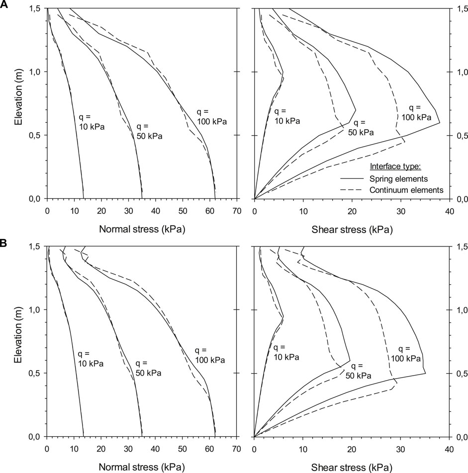
FIGURE 5. Comparison of load transfer results from backfill soil to facing panel using FLAC with (A) coarse mesh and (B) fine mesh: normal and shear stresses at the interface between the facing structure and backfill soil for a strength/stiffness reduction factor Ri = 0.8.

Figure 6 presents the same results but grouping by interface element type, so that the influence of meshing size can be compared. As can be observed, only small differences were obtained between coarse and fine mesh cases.

FIGURE 6

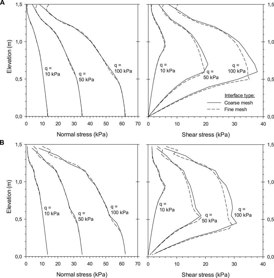
FIGURE 6. Comparison of load transfer results from backfill soil to facing panel using FLAC with (A) spring and (B) continuum interface elements with coarse mesh and fine mesh: normal and shear stresses at the interface between the facing structure and backfill soil for a strength/stiffness reduction factor Ri = 0.8.

Load transfer from backfill soil to facing panel using FLAC spring and continuum elements interfaces for two different strength/stiffness reduction factors (R_i = 0.3 and 1.0-rigid) are presented in Supplementary Figure S2 (Supplemental Material). As it can be observed, no fluctuations were obtained even for the rigid interface case.

For FLAC-PLAXIS comparison purposes, unglued interfaces were assumed, where the slip and/or opening behavior of interfaces is allowed, and the plastic shear displacement occurs after the shear stress exceeds a maximum shear strength controlled by the Coulomb shear–strength criterion. This is also compatible with the continuum material interface modeling using the CODE_BRIGHT FEM program (both 2D and 3D interface modeling).

Interface 2D Model and Properties With CODE_BRIGHT

Problem Definition: Soil Material Modeling Features

Continuum element interfaces were used in CODE_BRIGHT to simulate the soil-facing interaction with 18-mm-thick real zone. As in the previous cases, the structure (facing concrete panel) was modeled as linear elastic with elastic modulus of 32 GPa, Poisson ratio of 0.15, and a unit weight of 25 kN/m³. Soil material was modeled with Drucker–Prager failure criterion (i.e., circular cone in the principal stress space). In the program, the soil friction angle (ϕ) is defined with the critical state slope M-line in order to obtain correct shear strength. Using the Mohr–Coulomb failure criteria that circumscribe the Drucker–Prager failure criteria (see Supplementary Figure S3 in the Supplemental Material), strength is defined as follows:

$M=\frac{6\sin \varphi }{3-\sin \varphi }\left(\mathrm{triaxial}\mathrm{compression}\mathrm{state}\right)(14)$

For triaxial compression behavior of material, M_compression, that is, σ₁ > σ₂ = σ₃, where σ₁, σ₂, and σ₃ are the main stress states: σ₁ (major stress) ≥ σ₂ ≥ σ₃ (minor stress)). Assuming Drucker–Prager circle failure criteria that are inscribed within the Mohr–Coulomb failure criteria (see Supplementary Figure S3), the strength is defined as follows:

$M=\frac{6\sin \varphi }{3+\sin \varphi }\left(\mathrm{triaxial}\mathrm{extension}\mathrm{state}\right)(15)$

For triaxial extension behavior of material, M_extension, that is, σ₁ = σ₂ > σ₃. Thus, the stress states using the Mohr–Coulomb failure criteria can be defined by the M-parameter corresponding to the compression or extension condition.

As noted earlier, proper material constitutive modeling assuming M-values requires to determine the material state in terms of intermedia main stress scenario (i.e., σ₂ = σ₃ in compression, otherwise extension if σ₂ = σ₁). In common scenarios and in the ones assumed in the current study, the compression state corresponds to the most suitable case. Thus, soil model properties are the ones presented in Table 1, with proper choice of the compression M-parameter value: M_compression = 1.808.

Table 2 shows the same parameters as in Supplementary Table S1 but including M-values for compression, extension, and intermedia (M_average) case states. While results demonstrated that the interface material M-value falls within compression and extension values, default M_compression values were assumed for modeling the soil-facing interaction in this study.

TABLE 2

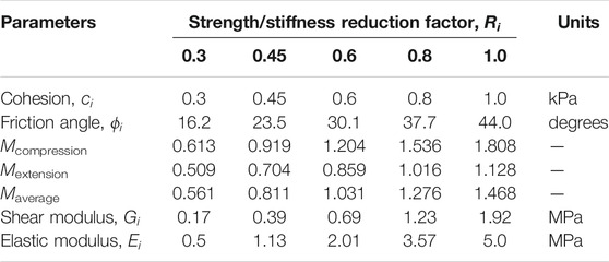
TABLE 2. Interface properties (related to E_soil = 5 MPa).

Effect of the Mesh Size and Element Type

Four different finite element 2D meshes were generated in CODE_BRIGHT: unstructured or irregular (but optimized) mesh with linear–triangular elements (Figure 7A), linear–triangular structured-mesh (Figure 7B), bilinear–quadrilateral structured-fine-mesh (Figure 7C), and bilinear–quadrilateral structured-coarse-mesh (Figure 7D). With these elements, it was possible to examine the effect of element size at the interface zone on the load transfer between the soil and facing structure.

FIGURE 7

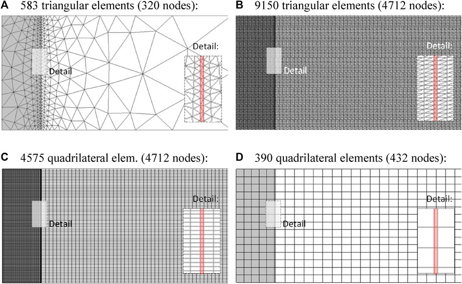
FIGURE 7. Four different finite element meshes for the same soil–structure interaction example using CODE_BRIGHT, with the same interface virtual thickness of ti = 18 mm: (A) unstructured mesh with linear–triangular elements, (B) linear–triangular structured-mesh, (C) bilinear–quadrilateral structured-fine-mesh, and (D) and bilinear–quadrilateral structured-coarse mesh.

Among these three meshes, the irregular mesh presented in Figure 7A had the highest element aspect ratio far from the analyzed soil–structure zone, but the optimized shape becomes finer with smaller aspect ratio in the interface zone. The structured fine mesh presented in Figure 7B has fine definition in all regions. However, triangular linear elements with analytical integration may not be the best ones because of the simple linear interpolation definition of this element type. This type of element did not work very well when shear strains occur with limits on volumetric strain development. Figures 7B,C have same number of nodes, even though the triangular mesh scheme has double the number of elements. However, both Figures 7C,D are for quadrilateral structured elements, which implies bilinear interpolation and numerical integration with quadrature of 4 Gauss points, and are probably better to perform soil–structure interactions for regular shear strain scenarios (despite the larger computational efforts required).

Settlement resulting under q = 100-kPa surcharge for the different meshes previously presented is shown in Figure 8 (R_i = 0.8). Despite the different meshing element types, good agreement was obtained between the four alternatives, for example, a maximum settlement value of 2.33 cm using triangular linear elements (both optimized and fine mesh cases) and 2.32 cm using quadrilateral bilinear elements.

FIGURE 8

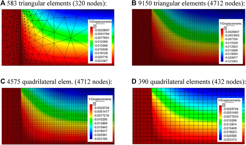
FIGURE 8. Settlements results (units in meters) using program CODE_BRIGHT with q = 100-kPa surcharge for the different meshes assumed: (A) unstructured mesh with triangular elements, (B) triangular structured-mesh, (C) quadrilateral structured-fine-mesh, and (D) and quadrilateral structured-coarse-mesh. Cases with ti = 0.018 m and Ri = 0.8.

Supplementary Figure S4 in the Supplemental Material presents the total shear strain evolution under q = 50 and 100-kPa surcharges (R_i = 0.8). Because results are scaled from 100-kPa surcharge in each meshing case, similar color distribution is obtained between meshing type with the exception of the quadrilateral coarse mesh (greater zone affected due to elements size). However, despite the similar responses in soil settlement with different mesh types used (Figure 8), a difference in strains from approximately 13% using the structured triangle mesh up to 19% using the structured quadrilateral fine mesh was obtained.

Results for load transfer from backfill soil to facing panel are plotted in Figure 9 for two cases of interface strength/stiffness reduction factors (R_i = 0.8 and R_i = 0.3). Despite variations noted in previous results, the triangular structured mesh improves results by avoiding the fluctuations in both normal and shear stress results when unstructured (but optimized) meshes are considered. Using quadrilateral elements, small differences were obtained between meshing size cases. These differences were even smaller when a softer (and weaker) interface reduction factor was selected.

FIGURE 9

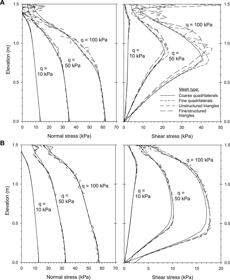
FIGURE 9. Load transfer from backfill soil to facing panel using program CODE_BRIGHT: normal and shear stresses at x = 0.509-m cross-section (i.e., at middle of the interface media; ti = 0.018 m) with different mesh type (unstructured or structured triangular, otherwise coarse or fine quadrilateral). Cases with (A) Ri = 0.8 and (B) Ri = 0.3.

Figure 10 presents the normal and shear load transfer from backfill soil to facing panel for different critical state slope M-parameter defining interface strength (see explanation in Section 3.2.1). Different results were obtained because of the M-value selected based on the triaxial state. Triaxial compression and extension state trends (i.e., M_compression and M_extension) generate a region of possible results. Differences between both compression and extension states are, however, not dramatic (e.g., similar differences were obtained using FLAC with the interface modeled by springs or continuum material; Figure 5). Results using an average value of M are also plotted (M_average) and these falls between both boundary triaxial states. The modeling results for compression and extension triaxial states using the continuum interface in CODE_BRIGHT and the continuum interface in PLAXIS and FLAC are presented in Figure 11 (R_i = 0.8 and R_i = 0.3 cases). Despite the fluctuations in the PLAXIS model response, similar results were obtained for FLAC and PLAXIS models used by Yu et al. (2014,2015). CODE_BRIGHT, PLAXIS, and FLAC results are shown to fall within the region bounded by compression and extension triaxial M-values results.

FIGURE 10

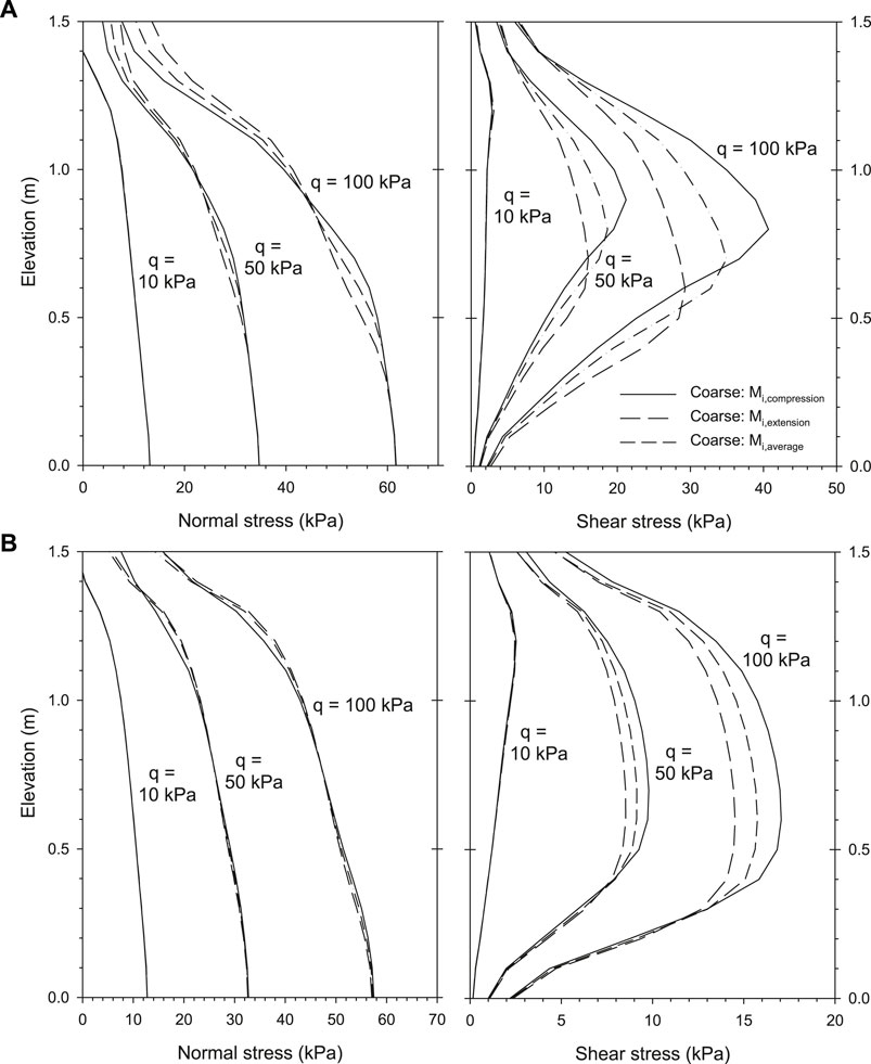
FIGURE 10. Load transfer from backfill soil to facing panel using program CODE_BRIGHT: normal and shear stresses with different Mi parameter (M_compression‒default assumed case—compared with M_extension and M_average). Cases with: (A) Ri = 0.8 and (B) Ri = 0.3.

FIGURE 11

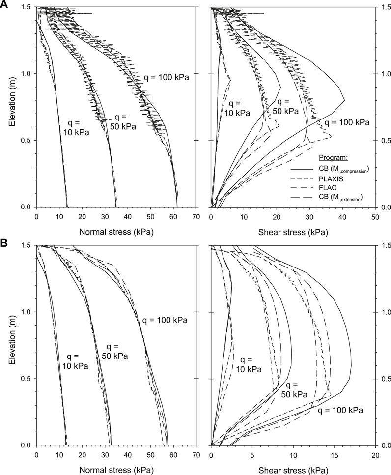
FIGURE 11. Load transfer from backfill soil to facing panel: comparison of normal and shear stresses using PLAXIS program (continuum elements interface; optimized mesh), FLAC (continuum elements interface; coarse mesh), and CODE_BRIGHT (both Mi-compression and Mi-extension scenarios performed). Cases with (A) Ri = 0.8 and (B) and Ri = 0.3.

Effect of the Strength/Stiffness Reduction Factor

Complementary to Supplementary Figure S4, Figure 12 shows the normal and shear stresses at the interface between the facing structure and backfill soil for three different strength/stiffness reduction factors investigated in CODE_BRIGHT modeling with quadrilateral coarse mesh elements (mesh case shown in Figure 7D). As before, the modeling results showed that increasing the strength/stiffness reduction factor R_i (i.e., increasing the interface stiffness) resulted in a smaller shear strains and relative displacements in the affected region: from approximately 13% for the rigid interface case to 22% for the R_i = 0.3 case. Note that, despite that the maximum displacement was similar at the right boundary contour (free displacement condition), the displacement distributions change markedly using the three strength/stiffness interaction factors.

FIGURE 12

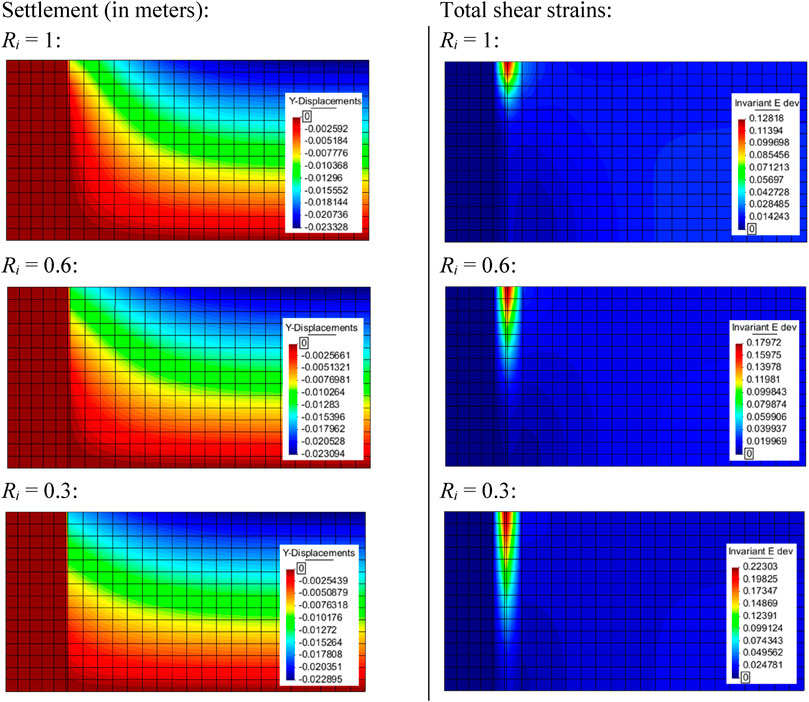
FIGURE 12. Settlement and total shear strain evolution using program CODE_BRIGHT with q = 100-kPa surcharge and different strength/stiffness interaction factors.

Results for the normal and shear stress transfer from backfill soil to facing panel using different interface strength/stiffness reduction factor and 100- and 50-kPa surcharge loading are found in Figure 13. Despite that the stress magnitude was different between the q-loading cases analyzed, very similar distributions were obtained. Significant variations in these distributions were obtained using the R_i values considered. Different R_i values influenced the resulting soil plastic zone (i.e., peak shear stress value location).

FIGURE 13

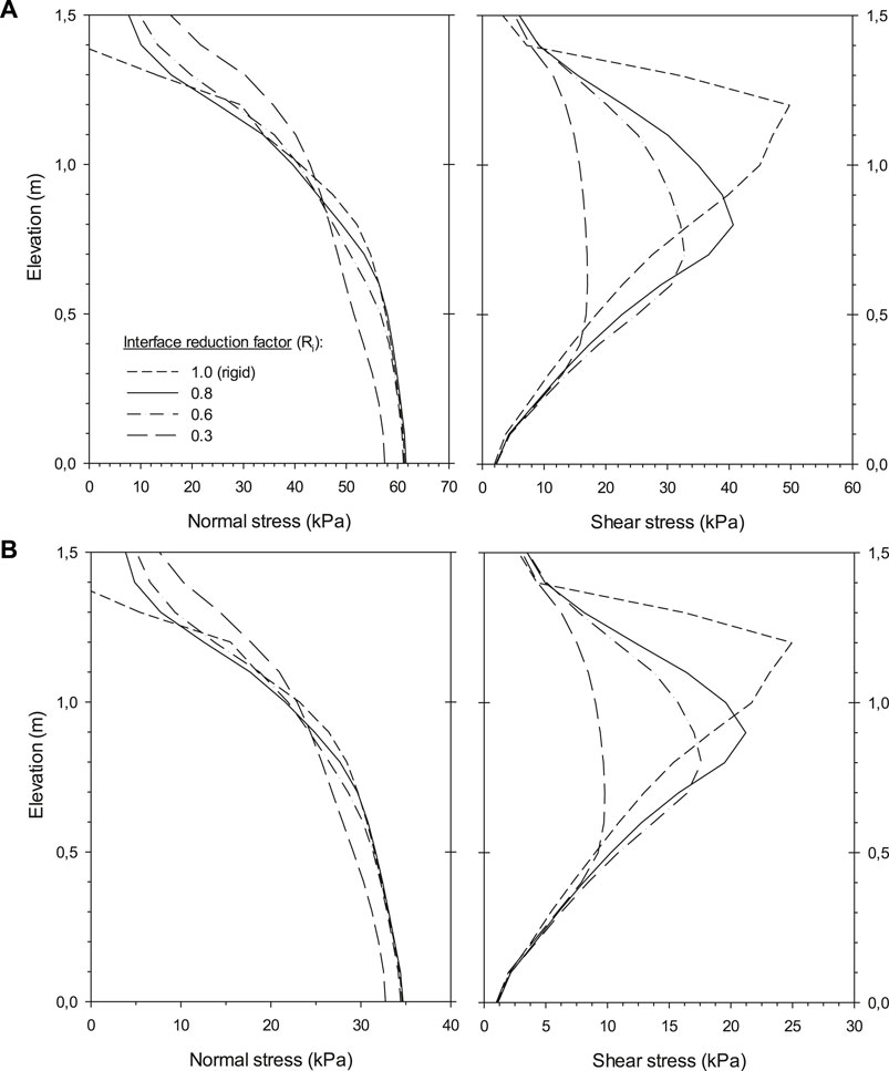
FIGURE 13. Load transfer from backfill soil to facing panel using program CODE_BRIGHT: comparison of normal and shear stresses with different interface strength/stiffness reduction factor (Ri values). Cases with (A) q = 100 kPa and (B) q = 50 kPa.

Effect of the Interface Thickness

Modeling of an 18-mm-thick (t_i) interface zone between dissimilar materials in full-height earth-retaining walls using continuum elements can be problematic because of the large difference in shape and size geometry between the different components within the retaining wall. It may be necessary to increase the interface thickness to accommodate other domain geometries. If this is the case, then the properties of the thicker interface must be adjusted to maintain the same (or similar) normal and shear strength/stiffness.

In this section, two interface thicknesses of t_i^* = 50 and 100 mm were examined using quadrilateral structured-coarse mesh case (Supplementary Figure S5 in the Supplemental Material, which correspond to complementary cases from Figure 7B—t_i = 18-mm-thick case). To keep the same interface stiffness, the new shear modulus (G_i^*) of the interface was calculated as follows:

$G_i^{\ast }=\left(G_i/t_i\right)t_i^{\ast }(16)$

where the Poisson ratio is the same for both interface thickness cases (i.e., v_i^* = v_i = 0.45), and the new oedometer modulus (E_oed,i^*) and elastic modulus (E_i^*) can be calculated using Eqs 4, 5, respectively, with the new shear modulus (G_i^*) and Poisson ratio (v_i^* = 0.45). Table 3 presents the equivalent interface properties for the case studies assumed and the additional interface thickness cases examined (as before, t_i^* = 50 and 100 mm).

TABLE 3

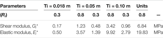
TABLE 3. Stiffness interface properties for t_i = 0.018 m (previous analyzed cases), t_i = 0.05 m and t_i = 0.10 m, related to E_soil = 5 MPa.

The computed settlements and shear strain (deviatoric invariant) for both interface thicknesses assumed (t_i = 0.05 m and t_i = 0.10 m) are presented in the Supplemental Material in Supplementary Figure S6 (case with R_i = 0.8) and Supplementary Figure S7 (R_i = 0.3). As shown, very similar responses were obtained for the three interface thickness cases (t_i = 18 mm case results presented in Figure 8D, Supplementary Figure S4 for R_i = 0.8, and Figure 12 for R_i = 0.3) under q = 50- and 100-kPa surcharge scenarios. As shown for previous cases, the reduction of the interface strength/stiffness interaction factor leads to an increase in the affected shear strain localization zone.

Results of normal and shear stress transfer from the backfill soil to the facing panel are presented in Figure 14 for the three interface thickness cases under q = 10-, 50-, and 100-kPa surcharge cases, and R_i = 0.8 and R_i = 0.3 interface strength/stiffness interaction cases. Results were obtained from a cross-section location at 9-mm distance from facing panel (i.e., at x = 0.509-m distance from left boundary), which corresponds to a line located within the t_i = 18-mm interface thickness case. The data show very similar responses for the three interface thickness cases.

FIGURE 14

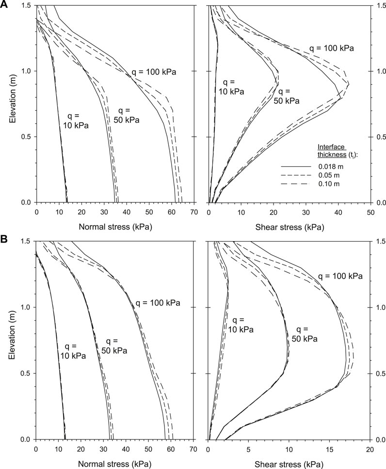
FIGURE 14. Load transfer from backfill soil to facing panel using program CODE_BRIGHT: normal and shear stresses for interface thicknesses of ti = 0.018, 0.05, and 0.10 m. Cross-section at x = 0.509 m. Cases with (A) Ri = 0.8 and (B) Ri = 0.3.

Supplementary Figure S8 in Supplemental Material presents the same previous results but for the cross-section location in the middle of each interface thickness: at 9-mm distance for ti = 18-mm-thick case, at 25-mm distance for ti = 50-mm-thick case, and at 50-mm distance for ti = 100-mm-thick case. It can be seen that there are practically no differences from the previous fixed cross-section location results.

The numerical results demonstrate that the increased interface thickness cases had a minor effect on the total vertical load at the interface between the facing and backfill soil if the equivalent interface stiffness was kept the same. Thus, a real interface zone between the dissimilar materials using continuum elements with a thickness greater than the virtual interface thickness using zero-thickness elements can be generated to model the soil–structure interactions and give similar numerical outcomes if the soil property values within the real interface zone are properly calculated based on the same interface stiffness.

CODE_BRIGHT 3D Modeling

Four different 3D models were generated to examine the soil-facing interactions using continuum elements matching the previous 2D results (Section 3.4). As in previous cases, different numerical meshes were assumed to detect any possible differences. Figure 15 presents the different meshes considered, from hexahedron coarse mesh case (related to previous structured quadrilateral 2D coarse mesh default case; Figure 7B), up to three different tetrahedron quality meshes.

FIGURE 15

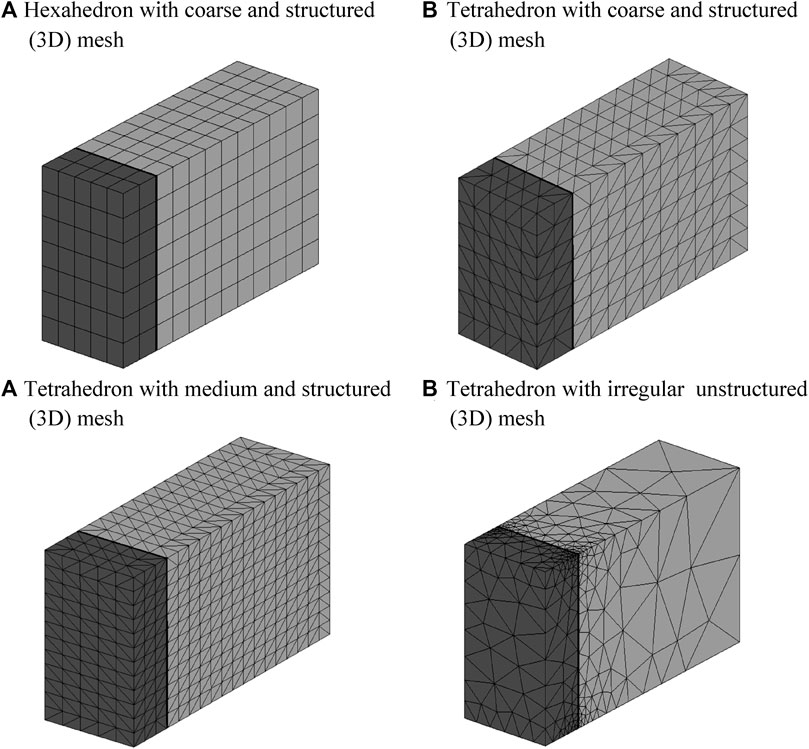
FIGURE 15. Two different finite element meshes for the same soil–structure interaction 3D example using program CODE_BRIGHT: (A) coarse structured (trilinear hexahedron elements) mesh and (B) optimized unstructured (linear tetrahedron elements) mesh with the same interface virtual thickness ti = 0.018 m.

Effect of the Mesh Size, Element Type, and Interface Reduction Factor

Figure 16 presents the resulting settlements under an applied 100-kPa surcharge. No practically different settlement responses can be seen for the four 3D modeling cases.

FIGURE 16

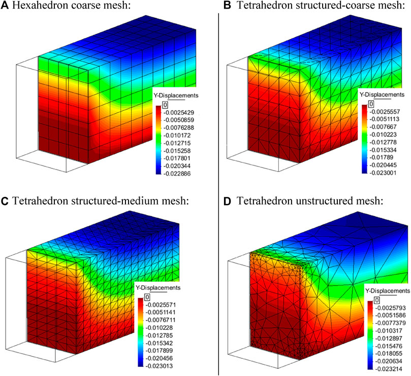
FIGURE 16. Settlement results (units in meters) under q = 100-kPa surcharge at top of soil zone: (A) hexahedron structured-coarse mesh, (B) tetrahedron structured-coarse mesh, (C) tetrahedron structured-medium mesh, and (D) tetrahedron unstructured irregular-mesh. Cases with ti = 0.018 m and Ri = 0.8.

The total shear strains are presented in Supplementary Figure S9 in the Supplemental Material. The higher strain values were similar for the four mesh cases (from approximately 16% to 18%). The figure shows that the cutting plane direction, which divides one hexahedron into two tetrahedrons, can deflect the shear strains to align with the element sides (compare Supplementary Figures S9A,B and see top-left elements, and then also in Supplementary Figure S9C). Despite this effect, only the case with unstructured meshing case (Supplementary Figure S9D) was judged to generate a major different response.

Figure 17 presents the normal and shear stresses transfer from backfill soil to facing panel at a cross-section located at 9-mm distance from facing (i.e., in the middle of the interface media; t_i = 0.018 m) using the previous 3D mesh types and quadrilateral structured 2D coarse meshing model case (cases with R_i = 0.8 and R_i = 0.3). Reasonably similar responses were obtained between 2D and equivalent 3D hexahedron structured coarse cases. Tetrahedron elements resulted in larger stress differences than for the hexahedron case, with largest differences using the unstructured mesh case (as in previous 2D modeling cases).

FIGURE 17

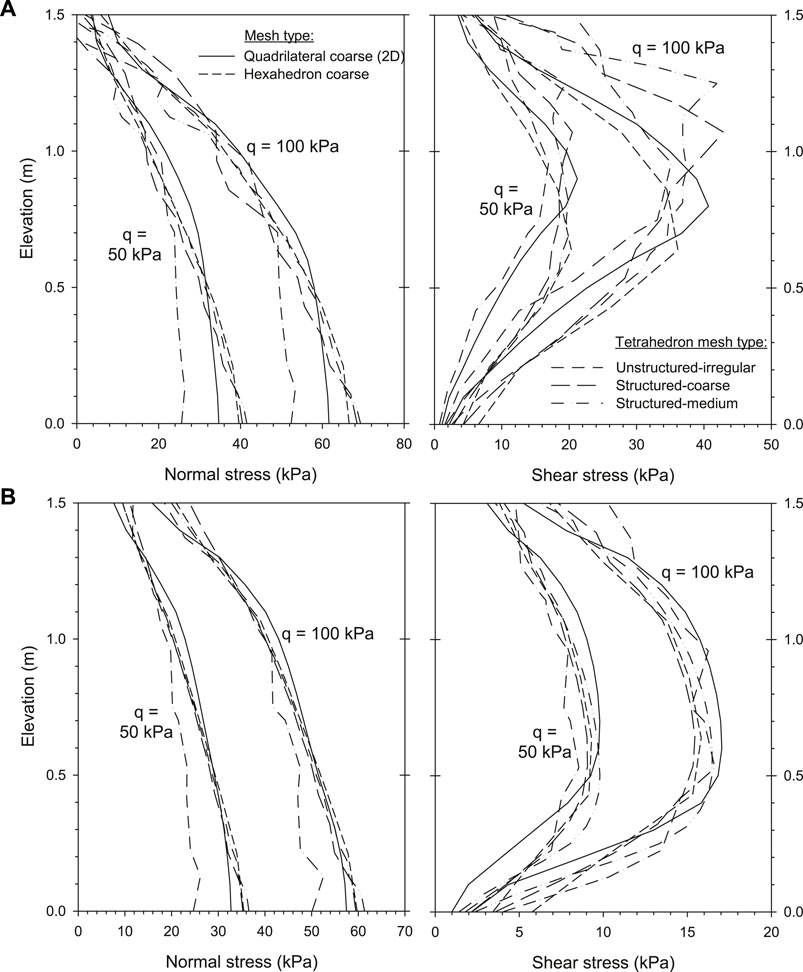
FIGURE 17. Load transfer from backfill soil to facing panel using program CODE_BRIGHT: normal and shear stresses at x = 0.509-m cross-section through the domain with 3D mesh type (coarse and optimized). Cases with (A) Ri = 0.8 and (B) Ri = 0.3.

Supplementary Figure S10 (Supplemental Material) presents the settlements under q = 100-kPa surcharge scenario using hexahedron elements with structured coarse mesh and R_i = 0.8 and R_i = 0.3 strength/stiffness interaction factor. As expected from earlier 2D cases (e.g., Figure 12), the influence on the volume of zone was different for each interface strength/stiffness case. Shear strains (deviatoric invariant) are shown in Supplementary Figure S11 for the conditions identified in the figures). As expected, higher strains were generated under the higher surcharge loading and also for the lowest interface strength/stiffness interaction factor.

Effect of the Interface Thickness

Two other thicknesses of the soil-facing interface were considered using the structured coarse mesh with hexahedron elements: t_i = 0.05 m and t_i = 0.10 m, matching previous 2D cases with the same material properties (Table 3).

Supplementary Figure S12 in Supplemental Material shows both mesh cases generated using the hexahedron structured coarse mesh type and methodology explained in Section 3.2.4.

Figure 18 presents the resulting settlements under 100-kPa surcharge using both interface thicknesses (i.e., t_i = 0.05 m and t_i = 0.10 m). As in the earlier 2D model cases analyzed, negligible differences were obtained using these two interface thickness value and the same R_i value.

FIGURE 18

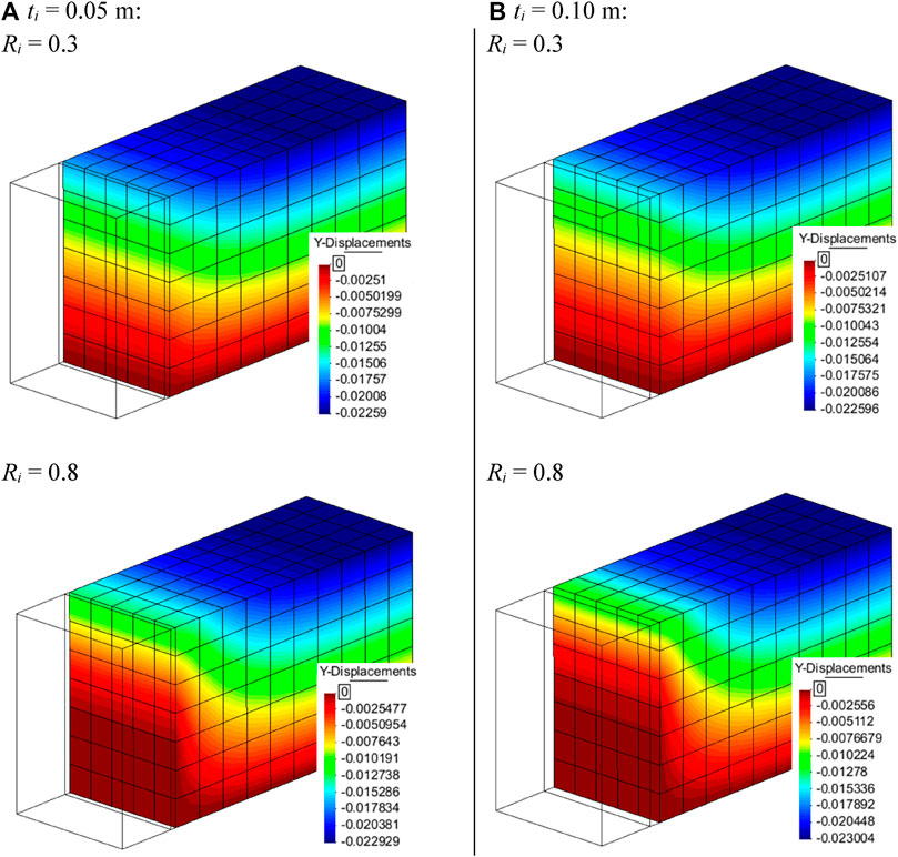
FIGURE 18. Settlement results (units in meters) under q = 100-kPa surcharge located at top of the soil zone and interface thickness (A) ti = 0.05 m and (B) ti = 0.10 m.

The shear strains obtained under 50- and 100-kPa surcharge are presented at Supplementary Figure S13 (R_i = 0.8) and S14 (R_i = 0.3). Again, practically no differences were obtained between both interface thickness cases for the same surcharge.

Finally, Figure 19 shows plots of normal and shear stress transfer from the backfill soil to the facing panel with R_i = 0.8 and R_i = 0.3 and three interface thicknesses (i.e., t_i = 0.018, 0.05, and 0.10 m) at a cross-section plane located at 9-mm distance from facing panel (i.e., in the middle of t_i = 0.018 m-thick case). The results of previous 2D model cases are included (previous Figure 7D—case). There is reasonable agreement among all cases. However, the greatest differences in trends were obtained between the 2D and 3D model cases. Nevertheless, variations were more or less within the same order of magnitude as in the element type comparison results (see Figure 17—elastic regime).

FIGURE 19

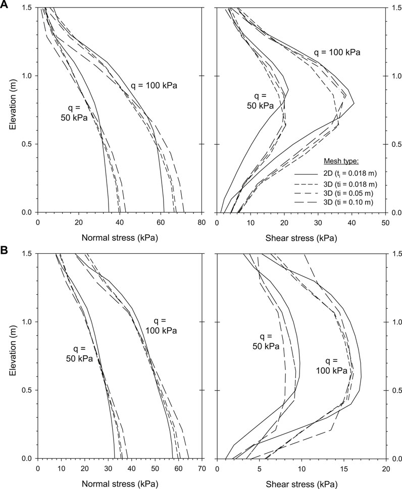
FIGURE 19. Load transfer from backfill soil to facing panel: normal and shear stresses using different interface thickness (ti = 0.018, 0.05, and 0.10 m): Cross-section at x = 0.509 m. Cases with (A) Ri = 0.8 and (B) Ri = 0.3.

Conclusions

This study presents numerical predictions of normal and shear stresses at the interface between soil and a concrete facing using two interface modeling approaches (i.e., zero-thickness elements and continuum elements) with equivalent interface properties based on the Mohr–Coulomb failure criterion. A small earth-retaining wall segment was used to demonstrate how the interfaces between the dissimilar materials can be modeled using both zero-thickness elements and continuum elements to capture soil–structure interactions. Based on the cases and conditions examined, the following conclusions are made:

• The finite element mesh had a minor influence on the predicted normal and shear stresses at the interface between the facing panel and backfill soil when using zero-thickness elements. Fluctuations of normal and shear stresses for the interface with continuum elements were observed once the soil within the interface zone reached plasticity (failed). However, the total vertical and horizontal loads at the interface from continuum elements generally agreed with those from zero-thickness or spring elements in both PLAXIS and FLAC models.

• For the interface with continuum elements, the finite element mesh with the lowest element aspect ratio (e.g., optimized mesh among the three meshes examined in this study) had the smallest normal and shear stress fluctuation amplitudes. Increasing the strength/stiffness reduction factor (i.e., increasing the interface stiffness) resulted in larger fluctuation amplitudes of normal and shear stresses when other conditions were the same.

• The real interface zone using continuum elements with a thickness greater than the interface virtual thickness from zero-thickness or spring elements can be used to generate similar numerical outcomes for finite element models with continuum elements and zero-thickness elements, if the equivalent interface stiffness is kept the same for both methods.

• The 3D modeling generated by program CODE_BRIGHT and assuming the interface defined by continuum elements gave good agreement with the 2D models and other interface methodologies using programs PLAXIS and FLAC.

Data Availability Statement

The raw data supporting the conclusions of this article will be made available by the authors, without undue reservation.

Author Contributions

Conception or design of the work: ID, SO, RB, AL, AJ. Models generation and model results: ID, SO. Analysis of results and interpretation: ID, SO, RB, AL, AJ. Drafting the article: ID, RB. Critical revision of the article: ID, SO, RB. Final approval of the version to be published: ID.

Conflict of Interest

The authors declare that the research was conducted in the absence of any commercial or financial relationships that could be construed as a potential conflict of interest.

Publisher’s Note

All claims expressed in this article are solely those of the authors and do not necessarily represent those of their affiliated organizations, or those of the publisher, the editors and the reviewers. Any product that may be evaluated in this article, or claim that may be made by its manufacturer, is not guaranteed or endorsed by the publisher.

Acknowledgments

The authors wish to acknowledge the support of the Department of Civil and Enviromental Engineering (DECA) of the Universitat Politécnica de Catalunya⋅BarcelonaTech (UPC), and the International Centre for Numerical Methods in Engineering (CIMNE) Severo Ochoa Centre of Excellence (2019-2023).

Supplementary Material

The Supplementary Material for this article can be found online at: https://www.frontiersin.org/articles/10.3389/fbuil.2022.842495/full#supplementary-material

References

Carter, J. P., Desai, C. S., Potts, D. M., Schweiger, H. F., and Sloan, S. W. (2000). Computing and Computer Modelling in Geotechnical Engineering. Proc. Int. Conf. Geotechnical Geol. Eng. (Geoeng2000) Melbourne 1, 1157–1252.

Google Scholar

Damians, I. P., Yu, Y., Lloret, A., Bathurst, R. J., and Josa, A. (2015b). “Equivalent Interface Properties to Model Soil-Facing Interactions with Zero-Thickness and Continuum Element Methodologies,” in Proceedings of the XV Pan-American Conference on Soil Mechanics and Geotechnical Engineering (XV PCSMGE): From Fundamentals to Applications in Geotechnics., Buenos Aires, Argentina, 15th – 18th November 2015, 1065–1072. doi:10.3233/978-1-61499-603-3-1065

CrossRef Full Text | Google Scholar

Damians, I. P., Bathurst, R. J., Josa, A., and Lloret, A. (2015a). Numerical Analysis of an Instrumented Steel-Reinforced Soil Wall. Int. J. Geomech. 15 (1), 04014037. doi:10.1061/(ASCE)GM.1943-5622.0000394

CrossRef Full Text | Google Scholar

Damians, I. P., Bathurst, R. J., Olivella, S., Lloret, A., and Josa, A. (2021). 3D Modelling of Strip Reinforced MSE walls. Acta Geotech. 16 (3), 711–730. doi:10.1007/s11440-020-01057-w

CrossRef Full Text | Google Scholar

Day, R. A., and Potts, D. M. (1994). Zero Thickness Interface Elements-Numerical Stability and Application. Int. J. Numer. Anal. Methods Geomech. 18, 689–708. doi:10.1002/nag.1610181003

CrossRef Full Text | Google Scholar

Desai, C. S., Zaman, M. M., Lightner, J. G., and Siriwardane, H. J. (1984). Thin-layer Element for Interfaces and Joints. Int. J. Numer. Anal. Methods Geomech. 8, 19–43. doi:10.1002/nag.1610080103

CrossRef Full Text | Google Scholar

Goodman, R. E., Taylor, R. L., and Brekke, T. L. (1968). A Model for the Mechanics of Jointed Rock. J. Soil Mech. Found. Div. 94, 637–659. doi:10.1061/jsfeaq.0001133

CrossRef Full Text | Google Scholar

Huang, B., Bathurst, R. J., and Hatami, K. (2009). Numerical Study of Reinforced Soil Segmental walls Using Three Different Constitutive Soil Models. J. Geotech. Geoenviron. Eng. 135 (10), 1486–1498. doi:10.1061/(asce)gt.1943-5606.0000092

CrossRef Full Text | Google Scholar

Itasca, (2011). FLAC: Fast Lagrangian Analysis of Continua, User’s Guide. Minneapolis, USA: Itasca Consulting Group, Inc.

Google Scholar

Montilla, E. A., Esquivel, E. R., Portelinha, F. M., and Javankhoshdel, S. (2022). “2D and 3D Numerical Study of Geosynthetic Mechanically Stabilized Earth GMSE walls,” in The Evolution of Geotech – 25 Years of Innovation, Open Access, 323–329. Availableat: www.taylorfrancis.comp.

Google Scholar

Ng, P. C. F., Pyrah, I. C., and Anderson, W. F. (1997). Assessment of Three Interface Elements and Modification of the Interface Element in CRISP90. Comput. Geotechnics 21, 315–339. doi:10.1016/s0266-352x(97)00020-7

CrossRef Full Text | Google Scholar

Olivella, S., Gens, A., Carrera, J., and Alonso, E. E. (1996). Numerical Formulation for a Simulator (CODE_BRIGHT) for the Coupled Analysis of Saline Media. Eng. Computations 13 (No.7), 87–112. doi:10.1108/02644409610151575

CrossRef Full Text | Google Scholar

PLAXIS (2012). Material Models Manual. PLAXIS B.V. Netherlands: Delft University of Technology. Availableat: http://www.plaxis.nl/.

Google Scholar

PLAXIS (2008). Reference Manual, 2D - Version 9.0. The Netherlands: PLAXIS B.V., Delft University of Technology. Availableat: http://www.plaxis.nl/.

Google Scholar

Potyondy, J. G. (1961). Skin Friction between Various Soils and Construction Materials. Géotechnique 11, 339–353. doi:10.1680/geot.1961.11.4.339

CrossRef Full Text | Google Scholar

Samtani, N. C., and Nowatzki, E. A. (2006). Soils and Foundations Reference Manual. Report No. FHWA-NHI-06-088. Washington, D.C: National Highway Institute, Federal Highway Administration.

Google Scholar

Won, M.-S., and Langcuyan, C. P. (2020). A 3D Numerical Analysis of the Compaction Effects on the Behavior of Panel-type MSE walls. Open Geosciences 12 (1), 1704–1724. doi:10.1515/geo-2020-0192

CrossRef Full Text | Google Scholar

Yu, Y., and Bathurst, R. J. (2017). Influence of Selection of Soil and Interface Properties on Numerical Results of Two Soil-Geosynthetic Interaction Problems. Int. J. Geomech. 17 (6), 04016136. doi:10.1061/(asce)gm.1943-5622.0000847

CrossRef Full Text | Google Scholar

Yu, Y., Damians, I. P., Bathurst, R. J., Lloret, A., and Josa, A. (2014). “Equivalent Interface Properties for FLAC and PLAXIS Models to Simulate Soil-Structure Interactions in MSE walls,” in Proceedings of the GeoRegina 2014. 67th Canadian Geotechnical Conference, Regina, Saskatchewan, Canada, September 28 ‒ October 1, 2014, 8p.

Google Scholar

Yu, Y., Damians, I. P., and Bathurst, R. J. (2015). Influence of Choice of FLAC and PLAXIS Interface Models on Reinforced Soil-Structure Interactions. Comput. Geotechnics 65, 164–174. doi:10.1016/j.compgeo.2014.12.009

CrossRef Full Text | Google Scholar