Computational characterization of visually induced auditory spatial adaptation

Introduction

The functional role of perception can be described as an inference about the sources of sensory signals in the environment. This process can be formalized by Bayesian probability theory that combines available sensory evidence (likelihood distribution) with prior knowledge (prior distribution) in making perceptual estimates (Knill and Richards, 1996; Rao et al., 2002). This study uses a Bayesian probabilistic model to computationally explain the adaptation of auditory spatial perception in response to auditory–visual conflict.

Recent studies have shown that Bayesian inference can account for human perception in a number of tasks. Many studies have explained observers’ visual perception within a Bayesian framework, with tasks ranging from speed detection (Stocker and Simoncelli, 2006b), to object perception (Kersten et al., 2004), color constancy (Brainard et al., 2006), and slant perception (Knill, 2003; Van Ee et al., 2003). An increasing number of studies have also used Bayesian models to account for human perceptual judgments across a range of multisensory tasks, including temporal numerosity judgment (Shams et al., 2005; Bresciani et al., 2006; Wozny et al., 2008), rate perception (Roach et al., 2006), oddity detection (Hospedales and Vijayakumar, 2009), self-motion perception (Fetsch et al., 2009, 2010; Butler et al., 2010), angular displacement (Jürgens and Becker, 2006), gravitoinertial force discrimination (Macneilage et al., 2007), and spatial localization (Körding et al., 2007; Rowland et al., 2007).

Whereas the aforementioned Bayesian models describe perceptual processes within a stationary setting, fewer studies have investigated the computational components of perception that undergo change as a result of adaptation. If the functional principles of sensory processing do indeed follow Bayesian computations, then the observed adaptive behavior should also be well characterized by changes in the Bayesian statistics. Given that the likelihood and prior distributions are the fundamental components of Bayesian inference, possible hypotheses are that adaptive behavior reflects: (i) changes in the prior probabilities, (ii) changes in the likelihood functions, (iii) or a combination of the two. Previous behavioral studies and model simulations appear to provide conflicting results about the perceptual component that undergoes change, and the results appear to be task dependent. Studies of sensory–motor adaptation in reaching (Körding and Wolpert, 2004), force estimation (Körding et al., 2004), and coincidence timing (Miyazaki et al., 2005) indicate that adaptation is associated with the update of the priors to match the distribution of recently experienced stimulus patterns. Adaptation of priors has also been reported for visual depth perception (Knill, 2007), convexity judgments (Adams et al., 2004), motion adaptation (Langley and Anderson, 2007), audio–visual integration (Van Wanrooij et al., 2010), and visual–tactile integration (Ernst, 2007).

However, other proposed models attribute adaptation to changes in sensory likelihoods. Stocker and Simoncelli (2006a), demonstrate that repulsive aftereffects observed after motion adaptation are inconsistent with a change in the prior distribution (that would produce attractive aftereffects), but instead are consistent with a sharpening of the likelihood distribution. Similarly, adaptation of the likelihood function has been proposed to qualitatively account for retinal contrast adaptation (Grzywacz and Balboa, 2002; Grzywacz and De Juan, 2003), speed adaptation (Barraza and Grzywacz, 2008), and auditory spatial recalibration (Sato et al., 2007). Yet one study of adaptation has found both repulsive and attractive kinds of changes in a temporal order judgment task depending on stimuli (Miyazaki et al., 2006). In one experiment, subjects judged the temporal order of two tactile stimuli, delivered one to each hand. When the distribution of presented stimuli had a larger proportion of right-hand-first intervals, subjects’ responses were biased in reporting right-hand-first as shown by shifts in the point of subjective simultaneity (PSS) of the cumulative psychometric function (and vice-versa for left-hand-first stimulus distributions). These results are in agreement with a Bayesian observer that updates a prior distribution in accordance with the distribution of stimulus presentations. However, in another experiment, when subjects were asked to judge the temporal order of audio–visual stimuli, the opposite effect was reported. The PSS was shifted in the opposite direction of that predicted by a Bayesian observer that updates the prior distribution. Thus, previous studies of calibration have reported different mechanisms of adaptation under different sensory conditions and tasks.

In this study, we are specifically interested in computationally characterizing perceptual adaptation in response to exposure to crossmodal sensory conflict. Acquiring information from multiple sensory organs enables the nervous system to perform self-maintenance and recalibration in response to detection of error in one of the senses. Such mechanisms can be critical in coping with exogenous changes in the environment or endogenous changes that occur as a result of development, injury, or stroke. Our study investigates a well-established example of crossmodally induced adaptation known as the ventriloquist aftereffect (VAE). After repeated exposure to simultaneous but spatially discrepant auditory and visual stimuli, the localization of an auditory stimulus when presented in isolation is shifted in the direction of the previously experienced visual offset (Canon, 1970; Radeau and Bertelson, 1974; Recanzone, 1998; Lewald, 2002). It has been argued that in the absence of information useful in determining which modality is biased, the nervous system does not always recalibrate when provided with cues having conflicting biases (Scarfe and Hibbard, 2011). However, the auditory spatial recalibration by vision (e.g., VAE) has been consistently shown to occur even when there is no information provided to the observers suggesting that the auditory estimates are biased, as is the case in this study. We aimed to gain insight into computational components of the perceptual process that are modified in the process of this adaptation. Because it has been previously shown that human localization of auditory and visual stimuli are consistent with a Bayesian causal inference observer (Körding et al., 2007; Wozny et al., 2010), we will use this model to characterize the perceptual components (sensory map, sensory noise, perceptual bias, etc.) for each individual observer before and after exposure to adapting stimuli. Simulation results (Figure 1) show that VAE can be qualitatively explained by either changes in the likelihood or changes in the prior distributions. Figure 1A schematically shows the stimuli used during the simulated adaptation period. The observers are exposed to simultaneous auditory and visual stimuli that are presented at a fixed spatial discrepancy from each other, here with sound to the left of the visual stimulus, at different positions along azimuth. The first row and second row show theoretical distributions of the prior (magenta), likelihood (blue), and the resulting posterior distributions (black) before and after exposure, respectively. The likelihood functions are shown for auditory stimuli at three arbitrary locations, −13°, 0°, and +13° of eccentricity (where 0° represents straight ahead location). The bottom row panels show the resultant change in the perceived location of sound at those locations. Each column represents one possible scenario in terms of changes mediating adaptation. In column B, the prior distribution is shifted to the right after exposure, which results in a rightward shift in perceived auditory locations, consistent with VAE (bottom row). In column C, the auditory likelihoods are shifted to the right. Here too, the perceived location of sounds is shifted rightward after exposure (shown in bottom row), consistent with VAE. Other changes or combinations of changes can produce distinct patterns of auditory aftereffects. One such example is shown in column D. In this example, before exposure the prior distribution is relatively flat. After exposure a prominent prior with a rightward bias emerges. This would cause asymmetric auditory shifts depending on the location of the prior mean relative to the testing locations. Therefore, VAE can be qualitatively explained by both a shift in priors and a shift in likelihoods or perhaps a combination of the two. Thus, to discover which computational changes in processing underlie this spatial adaptation phenomenon one needs to investigate it quantitatively by comparing psychophysical data with quantitative predictions of the different models.

FIGURE 1

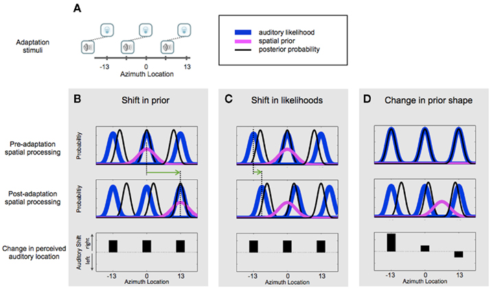
Figure 1. Possible computational mechanisms underlying ventriloquist aftereffect. (A) Schematic illustration of adapting stimuli. We present simulations for the case in which during exposure, the visual stimuli are to the right of the auditory stimuli by a fixed offset. This kind of exposure has been previously shown to result in a subsequent rightward shift in auditory localization. (B–D) depict three possible mechanisms of adaptation, and the resultant behavioral effects. Top row panels show distributions prior to exposure to discrepant auditory–visual stimuli shown in (A). Blue Gaussians show auditory likelihood distributions for three arbitrary horizontal locations, left (−13°), center (0°), and right (13°). Magenta Gaussian represents the prior distribution. Black Gaussians are the posterior estimates from the product of the likelihood and prior distributions. Middle panels show theoretical distribution changes after exposure. In scenario depicted in (B), the prior distribution is shifted to the right. The broken lines and green arrow highlight the shift in the prior distribution. The bottom panel shows the change in auditory spatial estimates (the max of posterior) after exposure (i.e., post-pre in the peaks of the black curves). Positive values denote a shift to the right. In scenario depicted in (C), adaptation causes a shift in likelihoods (blue curves). This mechanism produces the same behavioral effect as shown in (B) as seen in the bottom panel. Note that a smaller shift in likelihood (highlighted by the green arrow) results in the same magnitude of aftereffect as a larger shift in prior due to the relative widths of the distributions. In the scenario depicted in (D), before exposure the prior distribution is relatively flat (i.e., there is no bias for location), and after exposure a bias for a location to the right appears. This creates an asymmetrical pattern in aftereffect magnitudes across locations.

As mentioned earlier, it has recently been shown that human auditory–visual spatial localization judgments are remarkably consistent with a normative Bayesian causal inference model, where the observer infers the underlying causal structure of the environment based on the available evidence and prior knowledge (Körding et al., 2007). Because the causal inference model allows quantitative estimation of likelihoods and priors, this model can be used to empirically test which one(s) of these quantities undergoes change after adaptation. For each individual participant, model parameters were fitted to auditory–visual localization responses separately for pre-adaptation and post-adaptation data. This allowed us to test for statistically significant changes in the likelihood and prior parameters between the two phases. The key feature of this approach is that it allows simultaneous testing of all hypotheses of parameter changes without any a priori assumptions.

Materials and Methods

Participants and Apparatus

Twenty-four individuals (21 female) with a mean age of 20 (range 18–25) participated in the experiment. All participants reported normal or corrected-to-normal vision and normal hearing, and did not have any known auditory or neurological disorders. Each participant signed a consent form approved by the UCLA IRB. The participants were randomly assigned to one of two experimental groups, AV-adaptation (N = 12) and VA-adaptation (N = 12) as described below. The pre-test data from these subjects were part of a larger set of data previously published (Wozny et al., 2010). The participants in this study were the only participants subjected to the exposure conditions described below.

Participants sat at a desk in a dimly lit room with their chins positioned on a chin-rest 52 cm from a projection screen of stretched black linen cloth extending a vast portion of the visual field (134° width × 60° height). Behind the screen were nine free-field speakers (5 cm × 8 cm, extended range paper cone), symmetrically positioned around midline along azimuth, 6.5° apart, 7° below fixation. The visual stimuli were presented overhead from a ceiling mounted projector set to a resolution of 1280 × 1024 pixels. Figure 2 provides a schematic of the stimuli locations.

FIGURE 2

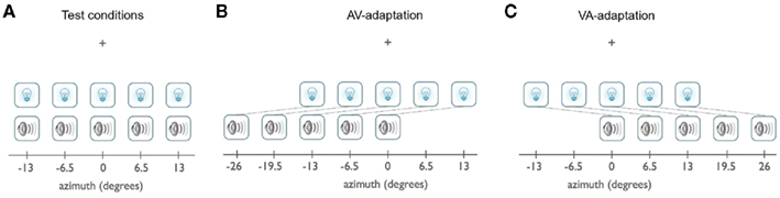
Figure 2. Spatial configuration of stimuli. Location of the visual and auditory stimuli during test phase (A) and during exposure phase for the AV-adaptation group (B) and exposure phase for the VA-adaptation group (C) are schematically shown. Here, the vertical locations of the visual and auditory stimuli are offset for illustration purposes; in the experiment they were vertically aligned at 7° below fixation. All combinations of visual and auditory stimulus locations were presented during test phases (A).

Stimuli

The visual stimulus was a white noise disk (0.41 cd/m²) masked with a Gaussian envelope of 1.5° FWHM, presented 7° below the fixation point on a black background (0.07 cd/m²), and presented for 35 ms. The visual stimulus was presented at a position coinciding with the center of one of the central five speakers behind the screen positioned at −13°, −6.5°, 0°, 6.5°, 13° along azimuth. Auditory stimuli were 35 ms ramped white noise bursts of 69 dB(A) sound pressure level at a distance of 52 cm and were newly generated on each trial. The speaker locations were unknown to the participants. The central five speakers were used as test locations for the auditory stimuli. The two eccentric speakers on each side were used during the adaptation period only.

Procedure

The experiment consisted of three phases: pre-adaptation test, adaptation, post-adaptation test. All three phases were performed in a single session lasting about 2 h. During pre-adaptation and post-adaptation test phases, participants performed a spatial localization task on unisensory as well as bisensory trials, which were randomly interleaved. These phases were each used for the estimation of the perceptual parameters (spatial maps, noise, bias, etc.) before and after adaptation. The adaptation period induced the VAE by exposing subjects to spatially offset auditory–visual stimulus pairs.

In order to familiarize participants with the task, each session started with a practice period of 10 randomly interleaved trials in which only an auditory stimulus was presented at a variable location, and subjects were asked to report the location of the auditory stimulus.

Practice was followed by 525 test trials that took about 45 min to complete. Fifteen repetitions of 35 stimulus conditions were presented in pseudorandom order. The stimulus conditions included five unisensory auditory locations, five unisensory visual locations, and all 25 combinations of auditory and visual locations (bisensory conditions). The locations of the stimuli were at −13°, −6.5°, 0°, +6.5°, +13° as shown in Figure 2A (positive is right of fixation). On bisensory trials, subjects were asked to report both the location of auditory stimulus and the location of visual stimulus in sequential order. The order of these two responses was consistent throughout the session, and was counter-balanced across subjects. Subjects were told that “the sound and light could come from the same location, or they could come from different locations.” As a reminder, a blue “S” or green “L” was placed inside the cursor to remind subjects to respond to the sound or light respectively. Probing both responses on bisensory trials allows us to assess the degree of sensory integration or segregation on a given trial.

Each trial started with a fixation cross, followed after 750–1100 ms by the presentation of the stimuli. After 450 ms, the fixation cross was removed and a cursor appeared on the screen vertically just above the horizontal line where the stimuli were presented and at a random horizontal location in order to minimize response bias. The cursor was controlled by a trackball mouse placed in front of the subject, and could only be moved in the horizontal direction. Participants were instructed to “move the cursor as quickly and accurately as possible to the exact location of the stimulus and click the mouse.” This enabled the capture of continuous responses with a resolution of 0.1°/pixel.

Following the pre-adaptation test, a top-up design was used for the adaptation period and post-adaptation test trials. During adaptation, a train of visual stimuli flashed on the screen at only one of the five central locations every 450 ms. Randomly, between the 5th and 15th presentation the flash got noticeably brighter (changed from 0.41 to 1.23 cd/m²), during which time the participant was to detect the change by clicking the mouse. If the change was caught prior to the next flash presentation, the stimulus moved to a new random location and the procedure continued. If the change was not detected or a false alarm was reported, the random sequence would start over in the same location and the location of the stimulus would not change until the brightness change was detected. The initial adaptation section lasted for 40 detections (8 detections per location). During adaptation phase, a simultaneous auditory stimulus was presented 13° either to the left (for the AV-adaptation group, Figure 2B) or to the right (for the VA-adaptation group, Figure 2C) of the visual stimulus, depending on the adaptation condition. Post-adaptation test segments consisted of 40 test trials randomly interleaved, followed by 10 randomly interleaved adaptation sequences (2 detections per location) until all 525 post-adaptation test trials were completed. Except for the ordering of the trials, the pre-adaptation and post-adaptation test phases were identical.

Causal Inference Model

We used a Bayesian causal inference model of multisensory perception (Körding et al., 2007) to probe any parametric changes in likelihood or prior distributions after inducing the VAE. In the causal inference model, the underlying causal structure of the environment is inferred based on the available sensory evidence and prior knowledge. Each stimulus or event s in the world causes a noisy sensation x_i of the event (where i is indexed over sensory channels). The sensory estimate for our task is the perceived location of the auditory and visual stimuli. The mapping from the world to sensory representations of the world is captured by the likelihood function p(x_i|s), which is the probability of experiencing sensation x_i as a result of event s occurring in the environment. We use a generative model to simulate experimental trials and subject responses by performing 10,000 Monte Carlo simulations for each condition. Each individual sensation is modeled using the likelihood function p(x_i|s). Trial-to-trial variability is introduced by sampling the likelihood from a normal distribution around the true sensory locations s_A and s_V, plus bias terms Δμ_A and Δμ_V for auditory and visual modalities, respectively. This simulates the corruption of auditory and visual sensory channels by independent Gaussian noise with standard deviation (SD) σ_A and σ_V respectively. In other words, the sensations x_A and x_V are simulated by sampling from the distributions shown in Eqs 1 and 2.

We assume there is a prior bias for the spatial location, modeled by a Gaussian distribution centered at μ_P. The SD of the Gaussian, σ_P, determines the strength of the bias. Therefore, the prior distribution of spatial location is

It is important to note that the posterior probability of event s is conditioned on the causal structure of the stimuli. For bisensory stimuli, the competing causal structures are shown in Figure 3, where the sensations could originate either from a common cause (C = 1, Figure 3 left, Eq. 4), or independent causes (C = 2, Figure 3 right, Eq. 5).

FIGURE 3

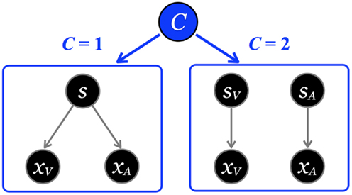
Figure 3. The causal inference model. Left: One cause can be responsible for both visual and auditory signals, x_V and x_A. Right: Alternatively, two independent causes may generate the visual and auditory sensations. The causal inference model infers the probability of a common cause (left, C = 1) vs. two independent causes (right, C = 2). The latent variable C determines which model generates the data.

Given that the likelihood and prior distributions are Gaussian, the resulting posterior distribution is also Gaussian, and the optimal estimates for the auditory and visual locations, and are taken as the maximum/mean of the posterior. These estimates are given in Eq. 6 for the common cause structure, and in Eq. 7 for the independent cause structure.

These are the optimal auditory and visual estimates given each causal structure. However, the causal structure is not known to the nervous system and also needs to be inferred based on sensory evidence and prior knowledge. This inference is formulated using Bayes’ Rule as follows:

The posterior probability of a single cause can be computed by:

where p_common is the prior probability of a common cause. The likelihood of experiencing the joint sensations x_A and x_V given a causal structure can be found by integrating over the latent variable s_i:

Again, since all integrands are Gaussian, the analytic solution is as follows:

The posterior probability of independent causes can then be calculated as:

At this point we have calculated the probability of each causal structure, and the optimal perceptual estimates assuming (i.e., under certainty about) each causal structure. The final stage is to obtain the perceptual estimates given the uncertainty in causal structure. If the goal of the nervous system is to minimize the mean squared error of the perceptual estimates, then the optimal solution would be to take the average of the estimates of the two causal structures, each weighted by their relative probability (Körding et al., 2007). This decision strategy is referred to as model averaging (Eq. 15).

However, as shown by Wozny et al. (2010), there are alternative decision-making strategies and cost functions that are adopted by some individuals. One alternative decision-making strategy is Bayesian model selection, which selects the auditory and visual estimates corresponding to the more probable causal structure:

The other alternative decision strategy we consider is probability matching. This is a stochastic strategy; on each trial a causal structure is selected with the probability matching its inferred probability. We simulate this strategy by randomly sampling from a uniform distribution on each trial (within a range from 0 to 1), and choosing the common cause model if its posterior probability is greater than the random sample (Eq. 17). An analogy of this process would be as follows: if there is a 70% chance of rain, and before one leaves the house one draws from an urn containing 100 balls labeled from 1 to 100, and then decides to take an umbrella if the drawn ball has a number below 70.

For each subject, we fitted model parameters to the participant’s response data using each of the three decision-making strategies described above (Wozny et al., 2010). We then chose the parameters and strategy that provided the best fit for each subject. Seven parameters were fitted simultaneously to the entire dataset (all 35 stimulus conditions) in an optimization search that maximized the likelihood of the data given the model parameters: Δμ_A, σ_A –the auditory likelihood mean offset and SD; Δμ_V, σ_V –the visual likelihood mean offset and SD; μ_P, σ_P –the prior mean and SD; and p_common – the prior probability of a common cause. A bounded version of Matlab’s fminsearch simplex algorithm was used for optimization. Parameter values were estimated separately for the pre-adaptation and post-adaptation test data. Paired two-tailed t-tests were used to test the differences between pre-adaptation and post-adaptation parameter values.

Results

For all figures and spatial parameters, 0° indicates straight ahead; negative and positive values denote left and right, respectively. Comparison between subjects’ post-adaptation and pre-adaptation responses in the unisensory auditory conditions showed significant VAE s in all five tested locations (Figure 4A). For each subject, the aftereffect magnitudes were calculated as the change (post-adaptation minus pre-adaptation) in mean subject auditory responses. In order to combine the data across the two adaptation groups, we negated the value of the aftereffect for the VA-adaptation group (to make their aftereffect values represented with a positive value). The mean magnitude of the shift in auditory spatial localization for each spatial location across all 24 subjects is shown in Figure 4A. As can be seen, there was a statistically significant adaptation effect at all tested locations.

FIGURE 4

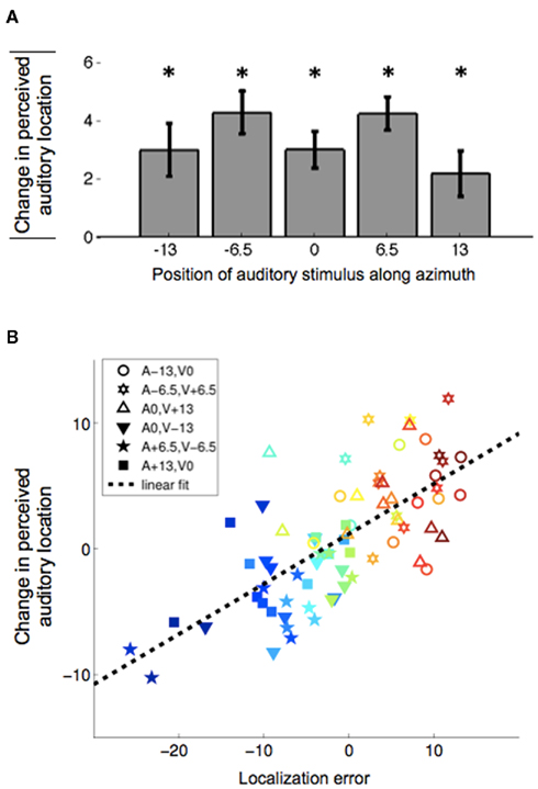
Figure 4. The magnitude of the observed adaptation effect. (A) Mean localization aftereffect magnitude at each tested location. Aftereffect magnitudes are measured as the difference post-adaptation minus pre-adaptation in mean subject auditory responses (N = 24). Here, positive aftereffects are defined as shifts in the direction of the visual stimulus offset presented during adaptation. *p < 0.05 two-tailed paired t-test, df = 23, Bonferroni corrected. (B) Scatter plot of aftereffect magnitude vs. pre-adaptation localization error. Aftereffects were measured as the post-adaptation minus pre-adaptation difference in the subjects’ mean auditory responses. Localization error was calculated at all bisensory pre-adaptation test locations with the same discrepancy (±13°) as that during exposure (3 data points per subjects × 24 subjects = 72 data points). The stimulus conditions are shown in the legend. The data points corresponding to the VA-adaptation and AV-adaptation groups are represented with filled and open symbols, respectively. The data points derived from the same subject share the same color. Dashed line shows a significant linear correlation of the data (r = 0.70, p < 0.0001).

Next, we examined the relationship between the auditory–visual interactions and the magnitude of the adaptation. We hypothesize that the recalibration is driven by the crossmodal error signal that occurs during the exposure presentations. Since we do not probe the auditory localization error during exposure, we must gather this information from the pre-adaptation data. As can be seen in Figure 4B, there is a linear correlation between the size of a subject’s aftereffect and the auditory localization error during bisensory pre-adaptation test trials with a discrepancy of 13° (the discrepancy that was presented during exposure). For each subject, there are three possible bisensory conditions that constitute either a positive or negative 13° discrepancy (consistent with exposure conditions for the two groups). For the AV-adaptation group (Figure 2B), the conditions are (A, V) = {(−13, 0); (−6.5, +6.5); (0, +13)}, and for the VA-adaptation group (Figure 2C), the conditions are (A, V) = {(0, −13); (+6.5, −6.5); (+13, 0)}. Localization error is defined as the subject’s auditory response minus the veridical location of the auditory stimulus during these bisensory trials. Aftereffect is defined as the subject’s mean post-adaptation test auditory response minus the mean pre-adaptation test auditory response at each of the three auditory alone conditions. The scatterplot of Figure 4B shows that the stronger the influence of the visual stimulus on auditory perception in bisensory trials (i.e., the stronger the auditory–visual interactions), the stronger the adaptation of the auditory spatial perception will be.

No significant correlation between the size of the aftereffect and either the SD of the auditory responses, or the fitted SD of the auditory likelihood function, σ_A, (see below) was found. It should be noted that the auditory–visual interaction is a non-linear function of both the auditory and visual SD, as well as the prior bias for perceiving a common source, p_common. Therefore, the absence of a linear correlation between a single variable and the aftereffect magnitude is not surprising.

The results discussed so far replicate the previous findings of VAE, and in addition suggest a direct role for auditory–visual interactions in producing the aftereffect. In order to investigate which perceptual components undergo change in this process and result in the aftereffect, we fitted the causal inference model described in the Methods section to each individual subject’s pre-adaptation and post-adaptation test data separately. All the model fits in this study were based on individual subject’s data (as opposed to group data) in order to test for statistically significant changes in parameters. Similar to our previous study of spatial localization (Wozny et al., 2010), the majority of subjects were fitted best by probability matching strategy: 18 (75%) matching; 3 (12.5%) selection; 3 (12.5%) averaging. Model fits to the pre-adaptation test group data for the 18 probability matching subjects are shown in Figure 5A for illustration purposes only in order to show the bimodal nature (i.e., having two peaks) of the response distributions and the ability of the model to capture these patterns. The post-adaptation test group data for probability matching subjects in the AV-adaptation group are shown in Figure 5B again for illustration purposes only. As can be seen, the response distributions in the unisensory auditory conditions (first row) are shifted to the right after adaptation. The model fitted the individual subject’s data very well, on average explaining 89% of the variance in the data (R² = 0.89 ± 0.05) across subjects and test phases¹. Although the precision of auditory localization was much worse than that of the visual localization in this experiment, and a previous study has suggested that auditory–visual integration may deviate from optimal when the difference in reliabilities of the two modalities is large (Bentvelzen et al., 2009) we do observe a pattern of behavior in all subjects that is highly consistent with Bayesian causal inference, as evident by the high values of goodness of fit.

FIGURE 5

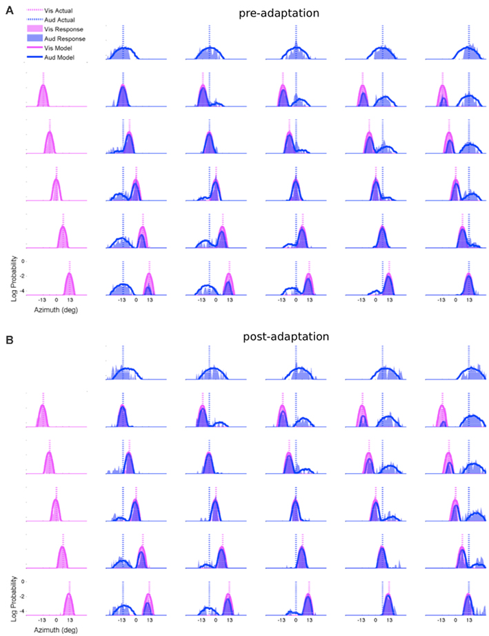
Figure 5. Subject group response distributions and the model fits. Observers’ marginal response log-probabilities for each stimulus condition are shown on the ordinate in shaded areas, and model fits are shown as superimposed solid lines. Vertical dotted lines show the true stimulus locations. The first row shows the five unisensory auditory conditions, with the sound location ranging from left to right along the azimuth as shown by the blue vertical dotted lines. The first column shows the five unisensory visual conditions, again with the stimulus position ranging from left to right as shown by the magenta vertical dotted lines. The remaining 25 panels in each figure show the bisensory conditions with both the visual and auditory response probabilities. (A) Pre-adaptation test data combined across 18 subjects who used the same decision-making strategy (probability matching). (B) Post-adaptation test data combined across subjects who were in the AV-adaptation group and used the same decision-making strategy (probability matching). For this group of eight subjects the unisensory auditory responses were shifted to the right after adaptation as can be seen in the first row.

The fitted parameter values were first submitted to a 2 × 2 repeated measures MANOVA with Adaptation (AV-adaptation, VA-adaptation) and Response Order (vision-first, audition-first) as between-subject factors and Test as a repeated measure (pre-adaptation, post-adaptation). Parameter estimate mean and SD for each Adaptation group are shown in Table 1. There was no significant main effect of response order, or interactions with response order (p > 0.05), indicating that the order of response did not have a significant impact on the results. However, there was a very strong Test × Adaptation interaction (p < 0.0001). Planned comparison analysis was then performed on each group’s data separately, using a paired two-tailed t-test between pre-adaptation and post-adaptation parameter values and these tests were corrected for multiple comparisons using Bonferroni correction for seven tests (α = 0.007). For both the AV-adaptation and VA-adaptation groups, the auditory likelihood offset parameter Δμ_A was the only parameter that was found to be significantly different between the two test phases (two-tailed paired t-test, df = 11, p = 0.0000 for both groups). All 24 subjects showed a shift in the auditory likelihood mean in the expected direction (i.e., toward the adapting visual offset). For the VA-adaptation group, there was a trend for increase in the spatial prior SD, σ_P, after adaptation (two-tailed paired t-test, df = 11, p = 0.01), however, it did not pass the Bonferroni test.

TABLE 1

Table 1. Sample mean ± SE parameter estimates for each adaptation group.

Figure 6 graphically displays the results using the same illustration scheme as in Figure 1. Actual parameters obtained from the data (shown in Table 1) are used to create the likelihood and prior distributions, and aftereffects magnitudes obtained from subjects’ responses (described above) are shown in the bottom row for each of the two adaptation groups. The exposure conditions are shown in the top row. To avoid crowding the figure, only the +13°, 0°, and −13° stimuli, likelihoods, and posteriors are shown, but aftereffects in the bottom row are shown for all five auditory stimulus conditions. Again, to avoid crowding the figure, the mean of the auditory likelihood functions are only shown for −13° auditory stimulus location. The green arrow denotes the likelihood shift to the right (panel A), or the left (panel B), and is shown again in the bottom panels. The aftereffect appears to be slightly larger at −6.5° and at +6.5° in panels A and B, respectively. However, this difference is not statistically significant. A previous study has suggested asymmetries in spatial generalization of the aftereffect (Bertelson et al., 2006), however, further investigation is required to determine whether the apparent asymmetry observed here is real and if so, what factor underlies it. One possible hypothesis for this trend is that the maximal aftereffect in each group corresponds to the location of maximal overlap in AV exposure as seen in Figures 2B,C (i.e., the location having AV exposure conditions on both left and right sides).

FIGURE 6

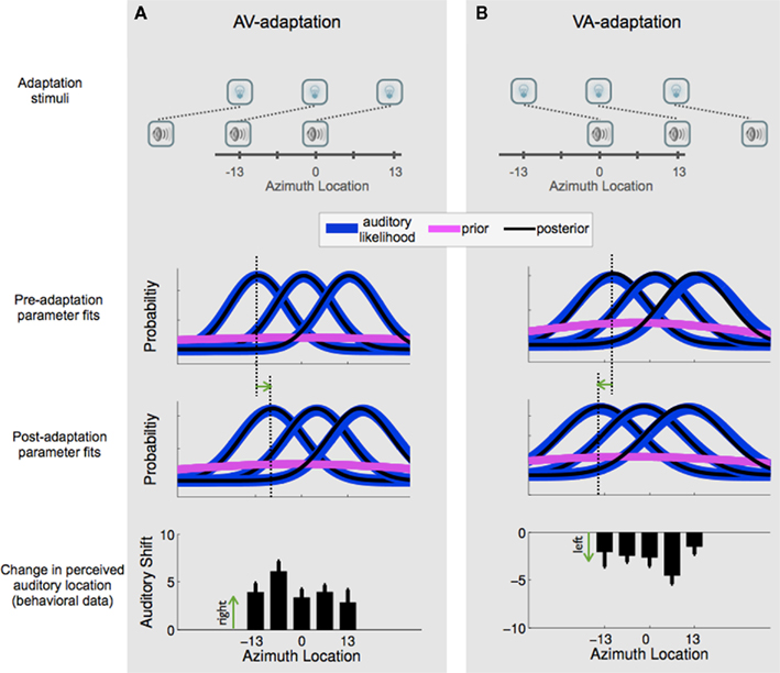
Figure 6. Graphical representation of the results. The top row schematically shows three of the five stimulus configurations for the AV-adaptation group (A) and VA-adaptation group (B). The Gaussian distributions in the second and third rows show the auditory likelihood, prior, and posterior distributions for the pre-adaptation and post-adaptation model fits, constructed with the parameters obtained from the data and shown in Table 1. The dashed lines highlight the mean of the likelihood distribution at one of the spatial locations (chosen arbitrarily for illustration purpose) before and after adaptation, and the green arrow shows the direction of shift in the auditory likelihood. The bottom row shows the actual aftereffects (mean ± SEM) measured from subject responses in the auditory alone conditions.

Discussion

We investigated auditory spatial adaptation using test phases in which auditory–visual and unisensory visual trials are interleaved with unisensory auditory trials. By probing both visual and auditory percepts in conditions with varying degrees of auditory–visual discrepancy we were able to quantify which of the underlying distributions underwent change during the adaptation process. Since most subjects had an almost flat spatial prior (∼40° SD), for the observed VAE to be explained by a change in prior, either a large change in prior mean or a narrowing of the prior variance would have been required. We did not observe any such changes. Instead, we find that the shifts in observers’ auditory localization are explained best with a shift in the mean of the auditory likelihood function as opposed to a change in the variance of the likelihood or a change in the position or strength of the prior bias.

Given that the distribution of spatial location of stimuli during test phases was uniform, it is unclear whether the relatively flat spatial prior observed in the test phases reflects a priori lack of strong spatial bias or whether it is quickly learned over the course of the pre-adaptation test phase. Note that the top-up design used for post-adaptation interleaving test trials with adaptation periods makes it unlikely that the test trials would entirely counteract the changes induced by adaptation. If adaptation had involved acquisition of a spatial bias as depicted in Figure 1D, this would have entailed a change in the variance and/or mean of the prior; which was not observed in the data. In regards to the prior bias for a common cause, p_common, one could expect an increase in this bias after adaptation due to exposure to repeated simultaneous auditory–visual presentations, or alternatively, a decrease in this bias due to exposure to spatially discrepant stimuli. However, we did not observe any evidence for change in p_common after adaptation.

Little is known about the longevity and robustness of VAE. Although we used a top-up design to minimize the possible erosion of the aftereffect by exposure to random auditory–visual discrepancies of the post-adaptation test trials, it is still possible that exposure to these test trials diminishes the adaptation effect and that the actual effect sizes both in terms of the shift in the auditory spatial localization and the underlying auditory likelihoods are much larger than we detected here.

Our findings are consistent with the theoretical work of Sato et al. (2007) on the VAE, and Grzywacz and Balboa’s (2002) framework for sensory adaptation in which adaptation is mediated by adjustment of parameters related to sensory representations. Our findings are also consistent with Stocker and Simoncelli (2006a) model that explains adaptation with a change in sensory likelihood functions. Their model accounts for unisensory repulsive aftereffects such as motion adaptation or tilt aftereffects by sharpening of the likelihood function. Our findings are also in line with the efficient coding theory of Clifford et al. (2000) in which repulsive tilt aftereffects are explained by adaptation in the sensory encoding.

Our results differ from those of some previous studies of adaptation that suggest a change in prior distributions. It should be noted that in many of these previous studies which have reported a pattern of adaptation consistent with change in the priors, no sensory, or sensorimotor conflict was present during adaptation. For example, Adams et al. (2004) showed that the “light-from-above” prior is modified after exposure to light from below stimuli conveyed through haptic cues. This study involved visual–haptic adapting stimuli that were congruent in terms of their underlying light-source.

Körding et al. (2004) showed that the prior expectation of force distributions can be adapted to arm perturbations over the course of an experiment. In their experiment, true visual feedback of finger movement was provided to the subjects at the end of the trial, without producing any conflicts between actual (proprioceptive) and perceived (visual) finger location. Miyazaki et al. (2005) showed that observers can adapt their sensory–motor coincidence timing to match the distribution of trial-by-trial target timing, consistent with updating the Bayesian prior. In this study there was no experimentally imposed conflict between the motor response and sensory feedback.

However, patterns of adaptation consistent with a change in priors have also been reported following exposure to sensory (or sensorimotor) conflict. For example, in the sensorimotor adaptation experiment by Körding and Wolpert (2004), conflicting visual feedback induced adaptive changes in reaching. The authors explain the shifts in motor behavior by the acquisition of a new prior distribution. It should be noted though, that in their model, they only incorporate visual evidence (likelihood) as the modality of sensation and the proprioceptive modality is not taken into account. An alternative explanation of the results would be a shift in the mean of the proprioceptive likelihood function, as opposed to a shift in the prior distribution. In a study by Miyazaki et al. (2006) which involved temporal order judgment of two tactile stimuli, the shift in perceived simultaneity after adaptation was consistent with a change in prior distribution of ordered stimuli. In contrast, in the same study, another experiment examining temporal order judgment of a sound and a flash showed a shift in perceived simultaneity in a direction opposite to that predicted by a change in the prior distribution (and consistent with previous reports of lag-adaptation (Fujisaki et al., 2004; Vroomen et al., 2004). The authors explain their findings in the audio–visual condition by incorporating a lag-adaptation mechanism, which is akin to a change in the underlying likelihood distribution. While the opposite patterns of adaptation found in these two experiments may be due to the unisensory vs. multisensory nature of stimuli, we believe it more likely that the different patterns of adaptation are due to the difference in perceived unity of the stimuli. In the unisensory tactile experiment, the two tactile stimuli were delivered to different hands. This large spatial separation together with the temporal discrepancy likely leads to the two stimuli being perceived as having stemmed from independent sources. In contrast, because of the relatively poor spatial acuity of sound, in the auditory–visual condition it is likely that the two stimuli were perceived as having a common source. Indeed in a previous study, we found that adaptation depends strongly on the perception of unity of the inducing stimuli (Wozny and Shams, 2011). In the unisensory tactile experiment, if the two stimuli were perceived to be independent of each other then the time difference (the lag) between the two stimuli would not amount to a sensory conflict. Therefore, in these studies in which exposure to sensory conflict appeared to lead to a change in priors, either the change in prior (vs. likelihoods) or the very presence of sensory conflict remain questionable.

The results in the current study provide increasing evidence that adaptation to conflicting sensory information results in changes to the likelihood functions. Therefore, altogether based on the existing data, one could hypothesize that the presence of conflicting sensory information of a perceived common source results in a recalibration of the underlying sensory likelihood functions, whereas, exposure to stimuli lacking sensory conflict would result a change in the prior distributions. Future studies should put this hypothesis to test in varying tasks and sensory and sensorimotor conditions.

Conflict of Interest Statement

The authors declare that the research was conducted in the absence of any commercial or financial relationships that could be construed as a potential conflict of interest.

Acknowledgments

We thank Stefan Schaal for helpful comments on the manuscript. David R. Wozny was supported by a UCLA graduate division fellowship and an NIH Neuroimaging Training Fellowship. Ladan Shams was supported by UCLA Faculty Grants Program, Faculty Career Development award.

Footnote

1. ^Goodness of fit was calculated using the generalized coefficient of determination formula described by Nagelkerke (1991). For the null model we use the maximum likelihood estimator of the linear model μ = xβ. The generalized R² is interpreted as the proportion of variance in the data that is explained by the model.

References

Adams, W. J., Graf, E. W., and Ernst, M. O. (2004). Experience can change the “light-from-above” prior. Nat. Neurosci. 7, 1057–1058.

Pubmed Abstract | Pubmed Full Text | CrossRef Full Text

Barraza, J. F., and Grzywacz, N. M. (2008). Speed adaptation as Kalman filtering. Vision Res. 48, 2485–2491.

Pubmed Abstract | Pubmed Full Text | CrossRef Full Text

Bentvelzen, A., Leung, J., and Alais, D. (2009). Discriminating audiovisual speed: optimal integration of speed defaults to probability summation when component reliabilities diverge. Perception 38, 966–987.

Pubmed Abstract | Pubmed Full Text | CrossRef Full Text

Bertelson, P., Frissen, I., Vroomen, J., and De Gelder, B. (2006). The after effects of ventriloquism: patterns of spatial generalization. Percept. Psychophys. 68, 428–436.

Pubmed Abstract | Pubmed Full Text | CrossRef Full Text

Brainard, D. H., Longère, P., Delahunt, P. B., Freeman, W. T., Kraft, J. M., and Xiao, B. (2006). Bayesian model of human color constancy. J. Vis. 6, 1267–1281.

Pubmed Abstract | Pubmed Full Text | CrossRef Full Text

Bresciani, J. P., Dammeier, F., and Ernst, M. O. (2006). Vision and touch are automatically integrated for the perception of sequences of events. J. Vis. 6, 554–564.

Pubmed Abstract | Pubmed Full Text | CrossRef Full Text

Butler, J. S., Smith, S. T., Campos, J. L., and Bülthoff, H. H. (2010). Bayesian integration of visual and vestibular signals for heading. J. Vis. 10, 23.

Pubmed Abstract | Pubmed Full Text | CrossRef Full Text

Canon, L. K. (1970). Intermodality inconsistency of input and directed attention as determinants of the nature of adaptation. J. Exp. Psychol. 84, 141–147.

Pubmed Abstract | Pubmed Full Text | CrossRef Full Text

Clifford, C. W., Wenderoth, P., and Spehar, B. (2000). A functional angle on some after-effects in cortical vision. Proc. Biol. Sci. 1705–1710.

Ernst, M. O. (2007). Learning to integrate arbitrary signals from vision and touch. J. Vis. 7, 7.1–14.

CrossRef Full Text

Fetsch, C. R., Deangelis, G. C., and Angelaki, D. E. (2010). Visual-vestibular cue integration for heading perception: applications of optimal cue integration theory. Eur. J. Neurosci. 31, 1721–1729.

Pubmed Abstract | Pubmed Full Text | CrossRef Full Text

Fetsch, C. R., Turner, A. H., Deangelis, G. C., and Angelaki, D. E. (2009). Dynamic reweighting of visual and vestibular cues during self-motion perception. J. Neurosci. 29, 15601–15612.

Pubmed Abstract | Pubmed Full Text | CrossRef Full Text

Fujisaki, W., Shimojo, S., Kashino, M., and Nishida, S. (2004). Recalibration of audiovisual simultaneity. Nat. Neurosci. 7, 773–778.

Pubmed Abstract | Pubmed Full Text | CrossRef Full Text

Grzywacz, N. M., and Balboa, R. M. (2002). A Bayesian framework for sensory adaptation. Neural Comput. 14, 543–559.

Pubmed Abstract | Pubmed Full Text | CrossRef Full Text

Grzywacz, N. M., and De Juan, J. (2003). Sensory adaptation as Kalman filtering: theory and illustration with contrast adaptation. Network 14, 465–482.

Pubmed Abstract | Pubmed Full Text | CrossRef Full Text

Hospedales, T., and Vijayakumar, S. (2009). Multisensory oddity detection as Bayesian inference. PLoS ONE 4, e4205. doi: 10.1371/journal.pone.0004205

Pubmed Abstract | Pubmed Full Text | CrossRef Full Text

Jürgens, R., and Becker, W. (2006). Perception of angular displacement without landmarks: evidence for Bayesian fusion of vestibular, optokinetic, podokinesthetic, and cognitive information. Exp. Brain Res. 174, 528–543.

Pubmed Abstract | Pubmed Full Text | CrossRef Full Text

Kersten, D., Mamassian, P., and Yuille, A. (2004). Object perception as Bayesian inference. Annu. Rev. Psychol. 55, 271–304.

Pubmed Abstract | Pubmed Full Text | CrossRef Full Text

Knill, D. C. (2003). Mixture models and the probabilistic structure of depth cues. Vision Res. 43, 831–854.

Pubmed Abstract | Pubmed Full Text | CrossRef Full Text

Knill, D. C. (2007). Learning Bayesian priors for depth perception. J. Vis. 7, 13.

Pubmed Abstract | Pubmed Full Text | CrossRef Full Text

Knill, D. C., and Richards, W. (1996). Perception as Bayesian Inference. Cambridge: Cambridge University Press, 516.

Körding, K., Beierholm, U. R., Ma, W., Quartz, S., Tenenbaum, J., and Shams, L. (2007). Causal inference in multisensory perception. PLoS ONE 2, e943. doi: 10.1371/journal.pone.0000943

Pubmed Abstract | Pubmed Full Text | CrossRef Full Text

Körding, K., Ku, S., and Wolpert, D. (2004). Bayesian integration in force estimation. J. Neurophysiol. 92, 3161–3165.

Pubmed Abstract | Pubmed Full Text | CrossRef Full Text

Körding, K., and Wolpert, D. (2004). Bayesian integration in sensorimotor learning. Nature 427, 244–247.

Pubmed Abstract | Pubmed Full Text | CrossRef Full Text

Langley, K., and Anderson, S. J. (2007). Subtractive and divisive adaptation in visual motion computations. Vision Res. 47, 673–686.

Pubmed Abstract | Pubmed Full Text | CrossRef Full Text

Lewald, J. (2002). Rapid adaptation to auditory-visual spatial disparity. Learn. Mem. 9, 268–278.

Pubmed Abstract | Pubmed Full Text | CrossRef Full Text

Macneilage, P., Banks, M. S., Berger, D. R., and Bülthoff, H. H. (2007). A Bayesian model of the disambiguation of gravitoinertial force by visual cues. Exp. Brain Res. 179, 263–290.

Pubmed Abstract | Pubmed Full Text | CrossRef Full Text

Miyazaki, M., Nozaki, D., and Nakajima, Y. (2005). Testing Bayesian models of human coincidence timing. J. Neurophysiol. 94, 395–399.

Pubmed Abstract | Pubmed Full Text | CrossRef Full Text

Miyazaki, M., Yamamoto, S., Uchida, S., and Kitazawa, S. (2006). Bayesian calibration of simultaneity in tactile temporal order judgment. Nat. Neurosci. 9, 875–877.

Pubmed Abstract | Pubmed Full Text | CrossRef Full Text

Nagelkerke, N. (1991). A note on a general definition of the coefficient of determination. Biometrika 78, 691–692.

CrossRef Full Text

Radeau, M., and Bertelson, P. (1974). The after-effects of ventriloquism. Q. J. Exp. Psychol. 26, 63–71.

Pubmed Abstract | Pubmed Full Text | CrossRef Full Text

Rao, R. P. N., Olshausen, B. A., and Lewicki, M. S. (2002). Probabilistic Models of the Brain: Perception and Neural Function. Cambridge, MA: MIT Press, 324.

Recanzone, G. (1998). Rapidly induced auditory plasticity: the ventriloquism aftereffect. Proc. Natl. Acad. Sci. U.S.A. 95, 869–875.

Pubmed Abstract | Pubmed Full Text | CrossRef Full Text

Roach, N. W., Heron, J., and Mcgraw, P. V. (2006). Resolving multisensory conflict: a strategy for balancing the costs and benefits of audio-visual integration. Proc. Biol. Sci. 273, 2159–2168.

Pubmed Abstract | Pubmed Full Text | CrossRef Full Text

Rowland, B., Stanford, T., and Stein, B. (2007). A Bayesian model unifies multisensory spatial localization with the physiological properties of the superior colliculus. Exp. Brain Res. 180, 153–161.

Pubmed Abstract | Pubmed Full Text | CrossRef Full Text

Sato, Y., Toyoizumi, T., and Aihara, K. (2007). Bayesian inference explains perception of unity and ventriloquism after effect: identification of common sources of audiovisual stimuli. Neural Comput. 19, 3335–3355.

Pubmed Abstract | Pubmed Full Text | CrossRef Full Text

Scarfe, P., and Hibbard, P. B. (2011). Statistically optimal integration of biased sensory estimates. J. Vis. 11. doi: 10.1167/11.7.12

CrossRef Full Text

Shams, L., Ma, W. J., and Beierholm, U. (2005). Sound-induced flash illusion as an optimal percept. Neuroreport 16, 1923–1927.

Pubmed Abstract | Pubmed Full Text | CrossRef Full Text

Stocker, A., and Simoncelli, E. (2006a). “Sensory adaptation within a Bayesian framework for perception,” in Advances in Neural Information Processing Systems, eds Y. Weiss, B. Schoelkopf, and J. Platt (Cambridge, MA: MIT Press), 18, 1291–1298.

Stocker, A. A., and Simoncelli, E. (2006b). Noise characteristics and prior expectations in human visual speed perception. Nat. Neurosci. 9, 578–585.

CrossRef Full Text

Van Ee, R., Adams, W. J., and Mamassian, P. (2003). Bayesian modeling of cue interaction: bistability in stereoscopic slant perception. J. Opt. Soc. Am. A Opt. Image Sci. Vis. 20, 1398–1406.

Pubmed Abstract | Pubmed Full Text | CrossRef Full Text

Van Wanrooij, M. M., Bremen, P., and John Van Opstal, A. (2010). Acquired prior knowledge modulates audiovisual integration. Eur. J. Neurosci. 31, 1763–1771.

Pubmed Abstract | Pubmed Full Text | CrossRef Full Text

Vroomen, J., Keetels, M., De Gelder, B., and Bertelson, P. (2004). Recalibration of temporal order perception by exposure to audio-visual asynchrony. Brain Res. Cogn. Brain Res. 22, 32–35.

Pubmed Abstract | Pubmed Full Text | CrossRef Full Text

Wozny, D. R., Beierholm, U., and Shams, L. (2008). Human trimodal perception follows optimal statistical inference. J. Vis. 8, 24.

Pubmed Abstract | Pubmed Full Text | CrossRef Full Text

Wozny, D. R., Beierholm, U. R., and Shams, L. (2010). Probability matching as a computational strategy used in perception. PLoS Comput. Biol. 6, e1000871. doi: 10.1371/journal.pcbi.1000871

CrossRef Full Text

Wozny, D. R., and Shams, L. (2011). Recalibration of auditory space following milliseconds of cross-modal discrepancy. J. Neurosci. 31, 4607–4612.

Pubmed Abstract | Pubmed Full Text | CrossRef Full Text