 Kyle A. Thompson1,2*
 Amos Branch2Tyler Nading3Thomas Dziura3Germano Salazar-Benites4Chris Wilson4Charles Bott4Andrew Salveson2Eric R. V. Dickenson1
- 1Water Quality Research and Development, Southern Nevada Water Authority, Henderson, NV, United States
- 2Carollo Engineers, Inc., Walnut Creek, CA, United States
- 3Jacobs Engineering Group, Inc., Englewood, CO, United States
- 4Hampton Roads Sanitation District, Virginia Beach, VA, United States
Industries occasionally discharge slugs of concentrated pollutants to municipal sewers. These industrial discharges can cause challenges at wastewater treatment plants (WWTPs) and reuse systems. For example, elevated total organic carbon that is refractory through biological wastewater treatment increases the required ozone dose, or even exceeds the capacity of the ozone unit, resulting in a treatment pause or diversion. So, alert systems are necessary for potable reuse. Machine learning has many advantages for alert systems compared to the status quo, fixed thresholds on single variables. In this study, industrial discharges were detected using supervised machine learning and hourly data from sensors within a WWTP and downstream advanced treatment facility for aquifer recharge. Thirty-five different types of machine learning models were screened based on how well they detected an industrial discharge using default tuning parameters. Six models were selected for in-depth evaluation based in their training set accuracy, testing set accuracy, or event sensitivity: Boosted Tree, Cost-Sensitive C5.0, Oblique Random Forest with Support Vector Machines, penalized logistic regression, Random Forest Rule-Based Model, and Support Vector Machines with Radial Basis Function Kernel. After optimizing the tuning parameters and variable selection, Boosted Tree had the highest testing set accuracy, 99.2%. Over the 5-day testing set, it had zero false positives and would have detected the industrial discharge in 1 h. However, setting fixed thresholds based on the maximum normal datapoint within the training set resulted in nearly as good testing set accuracy, 98.3%. Overall, this study was a successful desktop proof-of-concept for a machine learning-based alert system for potable reuse.
Introduction
Upsets in wastewater treatment plants (WWTPs) caused by transient industrial discharges can lead to exceedances of discharge permits. These upsets may have human health relevance at WWTPs that are water sources for advanced water treatment facilities (AWTFs) for potable reuse. Hence, proposed regulations for direct potable reuse in California would require: “on-line monitoring instrumentation at critical locations that measure surrogate(s) that may indicate a chemical peak” (SWRCB, 2021). However, the best strategy for analyzing the on-line data for accurate, proactive, real-time event detection has not yet been determined.
Event detection systems in wastewater and reuse are often separated into two levels of urgency: alert and alarm. An alarm would indicate a high degree of confidence that an event is occurring that could pose a risk to the public health, requiring the shutdown or diversion of water from the AWTF. Due to the high consequences of a false positive, alarms are generally set based on health-based, high levels on reliable sensors at critical control points. In contrast, an alert would indicate a reasonable probability (e.g., >50%) that an event may be occurring that requires attention or corrective action (e.g., increased ozone dose), but not a treatment shutdown. An alert would be more sensitive (i.e., triggered by smaller changes) compared to an alarm. Thus, an alert could trigger prior to an alarm during the early onset of an event, allowing time for corrective action and potentially preventing alarm-level changes to the treated water quality. To improve upon the status quo (i.e., data visualization monitored 24/7 by human operators), an alert system would need to detect an event before or equally as soon as it would become visually apparent to a human operator. An alert system with this capability would: (1) allow corrective action to be conducted more promptly or with greater confidence and justification, and (2) serve as a redundant measure to human monitoring.
Machine learning could be applied for alert systems in drinking water, wastewater, or reuse. Machine learning is the study of algorithms that “learn” from and make predictions based on data. Specifically, supervised machine learning (SML) creates mathematical models to predict outputs based on a set of labeled input data. In the context of wastewater and drinking water treatment facilities, input variables could include water quality variables, such as pH, and operational information, such as ozone dose. SML requires a training dataset to construct models and a testing dataset to evaluate and compare their accuracy. The training and testing sets must both have known outputs or labels for the models to be constructed and so their predictive accuracy can be compared in a meaningful way. Labels in the water context could be categories, such as “Normal” or an “Industrial Discharge Event,” or numerical, such as percentage of influent coming from industrial wastewater. Once the SML models have had their accuracy confirmed on the testing set with known labels, they can then be applied in the field on new data with unknown outputs. This training and testing procedure avoids overfitting, which is when an increasingly complicated model more closely matches the data upon which it was trained, but makes less accurate predictions with new data.
SML models could be more accurate for detecting and categorizing upsets than simpler alternatives, such as fixed thresholds on single variables (e.g., pH above eight indicating an industrial discharge event). SML models can recognize high outliers on a single variable—while other variables remain near average—as likely instrument malfunctions or maintenance rather than true water quality events. Contrastingly, if all variables differ from the average only slightly but in directions associated with a particular type of upset, SML models could detect low levels or early onsets not yet apparent to human operators or fixed threshold-based alarms. Additionally, unlike a fixed threshold on a single variable or calculated metric, many SML models can categorize data into three or more categories. This could be beneficial, for example, for distinguishing among industrial discharges from different sources. Furthermore, SML models are non-linear and more flexible than thresholds. That is, thresholds essentially categorizing anything within a rectangular space (or higher dimensional hyperrectangle, depending on the number of variables with thresholds) as Normal, and anything outside that rectangular space as an Event. In contrast, SML models, such as k-nearest neighbors or support vector machines with radial basis kernels, can draw boundaries as any variety of complex, curving shape as dictated by the data. SML has been studied for event detection within the water sector, for example, detecting increases in wastewater effluent at a drinking water intake or harmful algal blooms in a lake (Lin et al., 2018; Thompson and Dickenson, 2021). However, SML has not been studied for event detection within reuse treatment systems to the best of our knowledge.
There are many types of SML models–238 are available within the caret package in R, and thirty-five were screened in this study (Kuhn, 2019). Two families of machine learning models often applied for classification tasks include support vector machines and random forests. Support vector machines divide data into categories by maximizing the gap between the training examples (Suykens and Hornegger, 1999). When the training data are not fully separatable, support vector machines will instead minimize an error function. Furthermore, support vector machines only use the datapoints closest to the boundary, and these datapoints are called the support vectors. Support vector machines have outperformed neural networks for predicting Lake Erie water levels and total phosphorus in a river (Khan and Coulibaly, 2006; Tan et al., 2012).
Random forests take many random samples of the observations or input variables in the training dataset and decision trees are trained on each of these random samples (Breiman, 2001). The output of the random forest is the output selected by the plurality of these decision trees. Random forests have been applied for modeling surface water salinity as a function of other water quality variables and lake nutrients as a function of watershed characteristics (Wang et al., 2021; Khan et al., 2022). Boosted trees are related to random forests, but each new tree is trained based on the errors of the previous tree (Hatwell et al., 2021). Boosted trees have been applied to predict the flood susceptibility of tracts of land or groundwater well-productivity based on geographic data (Lee et al., 2017, 2019).
In this study, SML was applied to historical online sensor dataset from a utility as a proof-of-concept for SML-based alert systems. The online sensor data was provided by the Hampton Roads Sanitation District (HRSD). The analysis focused upon data collected within a secondary WWTP and in a downstream AWTF. HRSD has begun the Sustainable Water Initiative for Tomorrow (SWIFT), which will purify effluent from many of HRSD's WWTPs to recharge the Potomac Aquifer. The SWIFT Research Center (SWIFT RC) is a 3.8 million L/day demonstration-scale AWTF, which treats secondary effluent from a WWTP with a 5-stage Bardenpho process for biological nutrient removal. The SWIFT RC treatment train includes coagulation, flocculation, sedimentation, ozonation, biofiltration, GAC adsorption, and UV disinfection. SWIFT has a final treated TOC goal of 4 mg/L (Gonzalez et al., 2021).
HRSD has a robust industrial pretreatment program. For example, HRSD has identified sources of bromide, PFAS, acrylamide, and 1,4-dioxane discharged to its WWTPs (Nading et al., 2022). Permits, flow limitations, or innovative industrial pretreatment have been implemented to reduce the concentrations of these chemicals. Nonetheless, during the year 2020, approximately monthly spikes in online monitoring surrogates including secondary effluent TOC were observed at the SWIFT RC and caused pauses in production. These transient increases in TOC persisted through the flocculation/sedimentation process and appeared to be driven by dissolved organic carbon, not solely turbidity or particulate organic matter.
Elevated TOC has a cascading effect on both downstream treatment and water quality (e.g., higher ozone demand, higher TOC in the finished water, disinfection byproduct challenges, or faster GAC utilization). The chemical(s) and industrial source causing these events had not yet been identified at the time of this analysis. Since no TOC instruments were located at the WWTP influent, it was unknown whether these industrial discharge events were pass-through [i.e., organic substance(s) not fully removed by the WWTP] or inhibition [i.e., organic or inorganic substance(s) that affected the WWTP's removal of overall TOC]. Rapid detection of future events would be beneficial for (1) for corrective action, such as increased ozone dose or coagulant dose and (2) collecting water samples to assist with identifying the chemical signature of these events. Chemical analysis collected in the midst of such events could then provide clues about the responsible industry.
In this study, industrial discharges were detected using SML and hourly data from online instruments within HRSD's SWIFT RC and the upstream WWTP. A dataset (n = 758) containing thirty variables was provided to the models. Variables included raw wastewater conductivity, secondary effluent turbidity, and ozonation effluent UV transmittance. The dataset also included two examples of industrial discharges. Supervised machine learning was conducted using the caret package in R. Thirty-five different types of machine learning models were selected for screening based on their accuracy performing a similar classification task using online water quality data from a drinking water intake (Thompson and Dickenson, 2021). These 35 models were screened based on how accurately they detected an industrial discharge in the testing set using raw data and default tuning parameters. Six models were then selected for in-depth evaluation based on their training set accuracy, test set accuracy, or event sensitivity.
The six selected models were first checked for whether their test set accuracy depended on random chance. Next, preprocessing methods were evaluated for whether they improved the accuracy of the models by correcting for diurnal patterns or instrument drift. These preprocessing methods included calculating a rolling median and conducting principal component analysis. Next, relatively unimportant variables were omitted from the input data to see if the machine learning models would calculate faster without losing accuracy. Finally, the selected models were trained over a wider range of potential tuning parameter settings. Overall, this study was the first desktop proof-of-concept for a machine learning-based alert system for a potable reuse facility.
Methods
Thirty-five SML models were compared to detect suspected industrial discharge events at the SWIFT RC. These thirty-five models (Supplementary Table 1) were selected for screening based on their accuracy performing a similar classification task—detecting de facto reuse in surface water—using related online water quality instrumentation (Thompson and Dickenson, 2021). Models were trained and tested on real, full-scale, hourly data from 30 variables with a total sample size of 878 (about 37 days). Since the industrial source was unknown, datapoints were labeled “Normal” or “Event” based on retrospective expert human judgement. SML was conducted in R using the caret package. Caret is a package in the R programming language that enables around two hundred different previously published SML model types to be applied using similar code structure (Kuhn, 2008). Preprocessing methods were also compared to enhance model accuracy. SML performance was benchmarked against fixed thresholds on the input variables. This included both the actual alert thresholds at the AWTF, and alert thresholds trained based on the training set data used in this study. All raw data and R code for this study are included as Supplementary material.
Online instrumentation
Models were trained on 30 variables that included readings from online instruments or gauges. The location, measured variable, manufacturer, and model of each sensor are shown in Table 1.
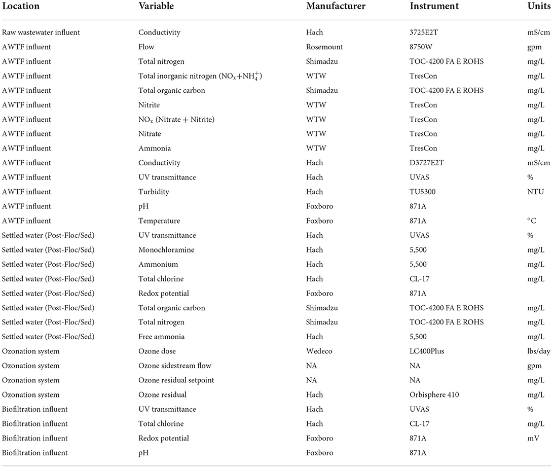
Table 1. Variables and instrument locations. AWTF influent could also be considered secondary wastewater effluent.
Data collection
Data was exported hourly on dates May 20th, 2019 through June 4th, 2019; June 15th, 2019 through June 21st, 2019; May 25th, 2020 through June 2nd, 2020; and October 17th, 2020 through October 21st, 2020 (Table 2). Suspected abnormal industrial discharges occurred during these periods on June 16th, 2019; June 1st, 2020; and October 18th, 2020. It was assumed these industrial discharges were from the same source or related enough to classify within the same SML output category. Missing data was assumed zero for ozone residual, ozone dose, and ozone output, since missing data for these variables was associated with shutdown of the ozonation system. For other variables (i.e., independent variables), missing data was assumed equal to the most recent previously measured value.
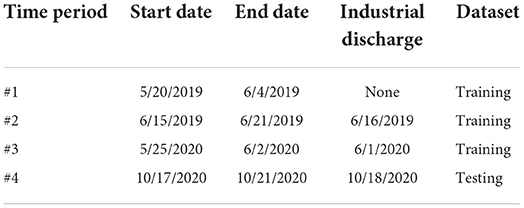
Table 2. Data time periods.
Supervised machine learning
The accuracy of certain types of SML models depends in part on random chance. For example, random forest models randomly select a subset of the observations or variables and then construct a decision tree based on this random subset. This process is repeated, typically hundreds of times, and an average or consensus is taken of the outputs of the decision trees. If the same random forest model is trained on the same data, but different subsets of data are selected for each tree, different testing set accuracies could result. In programming environments, randomness is simulated using random number generator algorithms such as Mersenne-Twister (Matsumoto and Nishimura, 1998). In the programming language R, numerical seeds can be provided to the random number generator. The same seed can be provided to enable reproducible results, or different seeds can be provided to simulate random replication. In this study, the seed was set to 1 unless otherwise noted to ensure reproducibility. For models selected for in-depth evaluation, seeds were set to integers from 1 to 30 or 1 to 100 to check whether the model accuracy was subject to random chance.
Most SML models have parameters that can be adjusted within the model that impact the learning process rather than being determined via the training. These parameters are called tuning parameters or hyperparameters. For example, k-nearest neighbors models assign new data to a class based on the most common label of the most similar datapoints. The tuning parameter k is the number of similar datapoints considered in the analysis. Tuning parameters are selected in a step in the machine learning process called cross-validation. In cross-validation, the training set is repeatedly split into smaller training and testing sets (sometimes called validation sets in this context). Models with different tuning parameter settings are trained on each internal training set and tested on each validation set. The tuning parameters that result in the best average performance on the validation sets are then selected and applied when making predictions on the final, fully separate testing test.
SML was conducted in R version 3.6.3 using the caret package (Kuhn, 2008). The caret package contains a set of programming functions that streamline the process of generating SML models. It allows a library of over 200 types of SML models to be trained and tested using similar coding grammar. Observations occurring during suspected abnormal industrial discharges were labeled Event. Other observations were labeled Normal. Data from May 20th, 2019 through June 2nd, 2020 (i.e., the first three of the four time periods, see Table 2) were used as a training set and contained two abnormal industrial discharge events: June 1st, 2019 and June 16th, 2019 (total sample size ntotal = 758, event sample size nevent = 66). Data from October 17th, 2020 through October 21st, 2020 was used as a testing set and contained one industrial discharge event: October 18th, 2020 (ntotal = 120, nevent = 28). Thus, the data was split ~86% training set, 14% testing set.
Models were screened on raw data (i.e., no preprocessing) using default tuning parameters in the caret package. The training set accuracy, testing set accuracy, event sensitivity, and total false alerts (i.e., false positives or Normal observations incorrectly predicted as Event), and p-value relative to the no information rate (NIR) were recorded for each model. Accuracy in the context of classification models means the overall percent of the dataset for which the model predicted the correct label. Sensitivity is how often the models were correct when the true answer was Event. The NIR is the accuracy that could be achieved by always assuming the most common label, which in this case was Normal. The NIR was 76.7%. The p-value that the testing set accuracy was above the NIR was calculated using the binomial confidence interval method (Clopper and Pearson, 1934; Kuhn, 2008).
The training set accuracy was internally cross-validated with 25 bootstraps (Kuhn, 2008). That is, 25 random samples were selected from the training set with the same total sample size as the original training set. These random samples were “with replacement,” i.e., it was possible for datapoints to be randomly selected more than once, or not at all, within each of the 25 samples. Random samples like these are called “bootstraps.” The bootstraps were then split 75:25 into training and validation sets, and the models were trained and validated 25 times using the 25 bootstraps. The average accuracy on the validation sets was then calculated and is referred to simply as “training set accuracy” below. This bootstrapped training set accuracy was used for selecting tuning parameters before final evaluation with the fully separate testing set.
Testing set accuracy was used as the primary metric of success in this study. Nonetheless, models from the screening phase were selected for further evaluation and tuning based on ranking in the top two for any of the following criteria: training set accuracy, testing set accuracy, or testing set event sensitivity. This was done because it was hypothesized that (1) models that were overfit (relatively high training set accuracy compared to testing set accuracy) might perform better on the testing set after tuning parameter optimization; or (2) models with high testing set sensitivity but many false positives might perform better after preprocessing to reduce noise.
The models selected for the in-depth evaluation phase were first trained and tested with one hundred distinct seeds to check whether their high performance was inherent to the model or due in part to random chance. Next, preprocessing techniques were tested to enhance model accuracy. Then, least important variables were iteratively omitted to investigate whether training time could be improved without loss in accuracy. Finally, models were cross-validated across a greater range of tuning parameter values.
Least important variables were identified using the variable importance (varImp) function from the caret package (Kuhn, 2008). The varImp function calculates importance differently depending on the type of the model. Regardless, variables are ranked and normalized on a scale of 0–100 based on their importance relative to the most important variable. Where the varImp function was not applicable, variables were omitted one at a time. If there was one variable whose omission resulted in equal or greater testing set accuracy, this variable was omitted. If there were multiple variables whose singular omission resulted in equal testing set accuracy, training set accuracy was used as a tiebreaker. If there were multiple variables whose singular omission resulted in equal testing and training set accuracies, one of these variable was selected at random for omission in the next iteration. This process was repeated until no variables could be omitted without a loss in accuracy.
Preprocessing
It was hypothesized that certain preprocessing methods could enhance model accuracy by reducing noise in the data or counteracting the effects of instrument drift. The four preprocessing methods assessed in this case study were: rolling median, difference from rolling median, principal component analysis (PCA), and lagging upstream sensors. The rolling median of the past three observations of each variable was calculated to reduce noise in the data and omit non-consecutive outliers. The difference between each observation and the median of the past day (i.e., 24 h observations) was calculated to account for the non-stationary nature of real wastewater data and optimize the data for detecting sudden changes (Supplementary Figure 1). Differences from the rolling median were provided to the models as variables both instead of and in addition to the raw data. PCA was conducted to promote diversity among the variables, considering that each principal component is perpendicular (non-correlated) with the others. PCA has previously been applied as a preprocessing technique for SML (Rodriguez et al., 2006). The PCA model was constructed based on the training set and then the scores for each principal component were calculated on the testing set.
Water traveling from the raw wastewater influent and the secondary wastewater effluent sensor locations had hydraulic residence times until reaching the post-flocculation settled water of 18 and 2 h, respectively. Thus, any changes or spikes from industrial discharges would be expected to begin at these sensor locations sooner, out of sync with the downstream sensors. Lagging the upstream sensors to align with the sensors in the settled water would provide many synchronized variables, while still providing a degree of advanced warning compared to the final purified water. So, lagging the raw wastewater influent and secondary wastewater effluent based on hydraulic residence time to match the settled water was explored as another preprocessing method.
Results
Water quality data
Descriptive statistics for Normal and Event data are shown in Supplementary Tables 2, 3, respectively. These tables include both train and testing set data. Timeseries for all variables are shown in Figures 1–3. Within these figures, panels #1, #2, and #3 are the training set and panel #4 is the testing set.
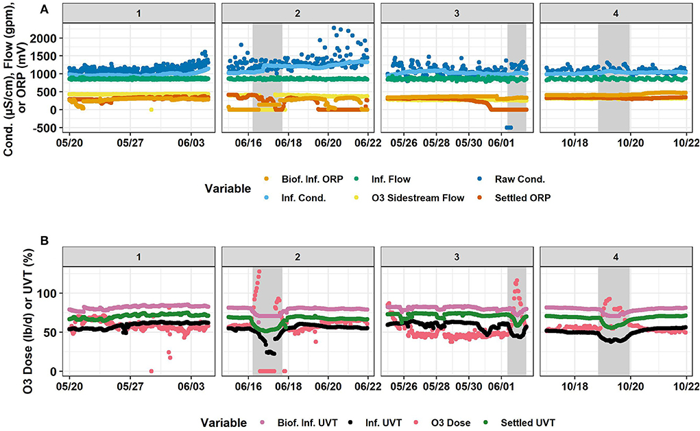
Figure 1. Timeseries of (A) biofilter influent ORP, influent flow, raw conductivity, influent conductivity, ozone sidestream flow, and settled water ORP, and (B) biofilter influent UVT, influent UVT, ozone dose, and settled water UVT. Horizontally, panels are separated into the four time-segments analyzed. #1 and #2 are in 2019. #3 and #4 are in 2020. #1, #2, and #3 were used for the training set and #4 was the testing set. Gray shaded areas represent abnormal industrial slug events. Source: Salveson et al. (Forthcoming). Reprinted with permission. © The Water Research Foundation.
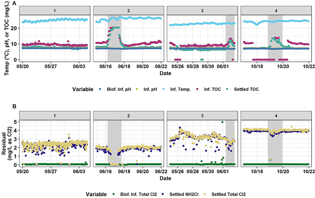
Figure 2. Timeseries of (A) biofilter influent pH, influent pH, influent temperature, influent TOC, and settled water TOC and (B) biofilter influent total chlorine, settled water monochloramine, and settled water total chlorine. Horizontally, panels are separated into the four time-segments analyzed. #1 and #2 are in 2019. #3 and #4 are in 2020. #1, #2, and #3 were used for the training set and #4 was the testing set. Gray shaded areas represent abnormal industrial slug events. Source: Salveson et al. (Forthcoming). Reprinted with permission. © The Water Research Foundation.
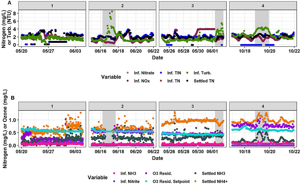
Figure 3. Timeseries of (A) influent nitrate, influent total inorganic nitrogen, influent turbidity, influent nitrogen oxides, influent total nitrogen, and settled water total nitrogen and (B) influent ammonia, ozone residual, settled water ammonia, influent nitrite, ozone residual setpoint, and settled water ammonium. Horizontally, panels are separated into the four time-segments analyzed. #1 and #2 are in 2019. #3 and #4 are in 2020. #1, #2, and #3 were used for the training set and #4 was the testing set. Gray shaded areas represent abnormal industrial slug events. Source: Salveson et al. (Forthcoming). Reprinted with permission. © The Water Research Foundation.
Machine learning results
Based on the screening results, six models were selected for further evaluation: Cost-Sensitive C5.0 (C5.0Cost), Oblique Random Forest with discriminative nodes based on linear support vector machines (ORFsvm), Penalized Logistic Regression (plr), Support Vector Machines with Radial Basis Function Kernel (svmRadial), Random Forest Rule-Based Model (rfRules), and Boosted Tree (bstTree) (Table 3). Lagging the raw wastewater influent and secondary effluent variables resulted in less testing set accuracy for all six models. This could be because lagging reduced the training set sample size by n = 54 or about 7%. Eighteen sample points had missing data at the start of each of the three non-consecutive periods. The lower testing set accuracy after lagging may also have been partly due to the increased percent accuracy loss per error with the smaller testing set (n = 102 instead of n = 120).
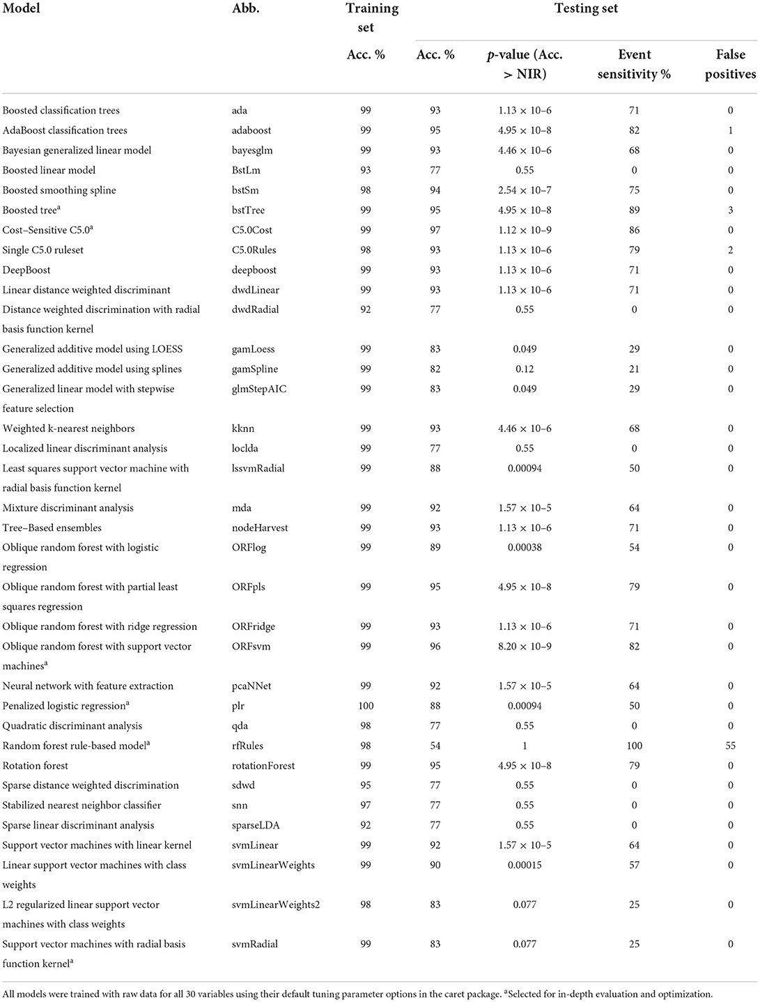
Table 3. Model screening results.
Cost-Sensitive C5.0
C5.0Cost is a decision tree algorithm with adaptive boosting and efficient pruning algorithms for relatively fast calculation (Nolan, 2002; Peng et al., 2020). C5.0Cost had the highest testing set accuracy in the screening, 96.7% (Table 3). The testing set accuracy of this model did not depend on the seed. Preprocessing by PCA, the rolling median, or the difference relative to the rolling median did not increase testing set accuracy. Biofilter influent pH was identified as the least important variable, but omitting it reduced testing set accuracy. C5.0Cost has four tuning parameters: (1) whether the model is based on associative rules or decision trees, (2) the number of boosting iterations (i.e., trials), (3) the cost of errors, (4) and whether an internal variable section process called winnowing is used. A rules-based model without winnowing with 20 trials (boosting iterations) and cost = 1 (weight of one assigned to errors) was selected based on the training set accuracy. Trials over 20 or cost >1 would have led to overfitting, with similar training set accuracy but lower testing set accuracy (Supplementary Figure 2). C5.0 had zero false positives and four false negatives, which were consecutive at the beginning of the industrial discharge event (Figure 4). Thus, there would have been a 4 h delay between the first hourly datapoint considered to be part of the event and the automated alert (i.e., first true positive) (Table 4).
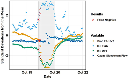
Figure 4. Testing set results of C5.0Cost. Using all raw data with default tuning parameters (Cost = 1, trials = 20, model = rules, winnow = false). The shaded gray area represents the Event. Red X's indicate false negatives. The four most important variables (biofilter influent UVT, influent turbidity, influent UVT, and ozone sidestream flow) are shown and scaled by training set standard deviation and mean. Source: Salveson et al. (Forthcoming). Reprinted with permission. © The Water Research Foundation.
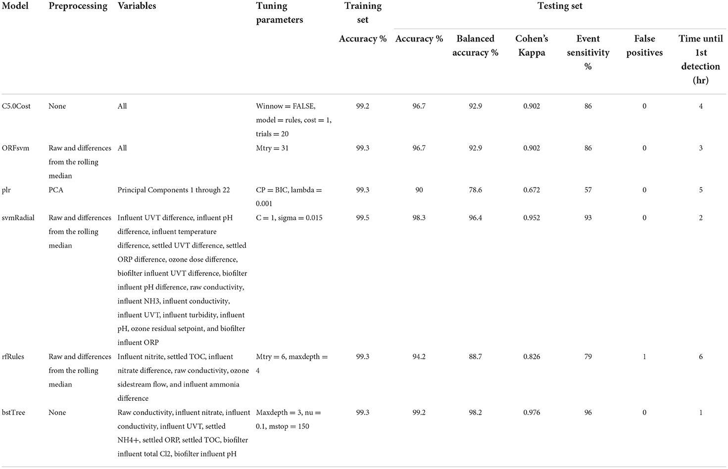
Table 4. Summary and performance metrics of six optimized models with their most beneficial preprocessing techniques, optimal tuning parameters, and final variable selection. Testing set false negatives and false positives are out of a sample size of n = 120 or 5 days of hourly data.
Oblique random forest with support vector machines
Oblique random forest is a decision tree ensemble in which multivariate trees learn optimal split directions at internal nodes using linear discriminative models (Menze et al., 2011). ORFsvm is a type of oblique random forest in which node splitting rules are based on support vector machines (Poona et al., 2016). ORFsvm had the second highest testing set accuracy in the screening, 95.8% (Table 3). Retraining the model with 100 distinct seeds revealed that the testing set accuracy of this model was stochastic, i.e., depending on random chance (Figure 5A). Nevertheless, the mean testing set accuracy was 95.5 with 0.1% standard error, so this model would indeed rank second in testing set accuracy on average. Training the model on both the raw data and the differences from the rolling median increased the ORFsvm median testing set accuracy to 96.7%, tying C5.0Cost (Figure 5B). The four errors in ORFsvm with this preprocessing were all false negatives, three of which were at the start of the event, and one at the end of the event. Thus, in practice, this model would have detected the event in about 3 h, sooner than C5.0Cost. ORFsvm had one tuning parameter, mtry, which is the number of randomly selected variables for each decision tree within the ensemble. However, varying mtry from 1 to 60 had no impact on training or testing set accuracy when using both raw data and differences from the rolling median.
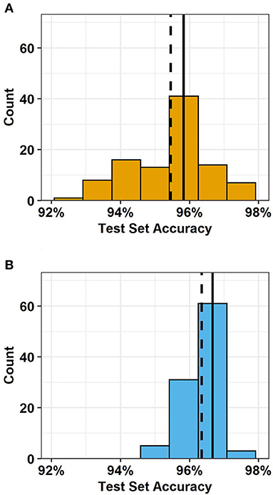
Figure 5. Distribution of testing set accuracy of ORFsvm. All variables and with default tuning parameters over 100 distinct seeds, with (A) raw data and (B) both raw data and differences from the rolling median. The solid vertical black lines represent the median and the dashed vertical black lines represent the mean. Source: Salveson et al. (Forthcoming). Reprinted with permission. © The Water Research Foundation.
ORFsvm had a relatively slow training calculation time, about 6 min per tuning parameter setting and seed iteration with 60 variables (all raw data and differences from rolling median). The varImp() function was not applicable for ORFsvm, and so could not be used to omit variables. Considering ORFsvm accuracy was stochastic, a sample size of at least 30 seed iterations would be required to determine if small changes in accuracy were the result of variable omission or random chance. Thus, a one-at-a-time variable omission procedure would have taken at least 1 week of computation time, and potentially months or over a year depending on the number of variables omitted. So, ORFsvm was not evaluated for variable omission. While not necessarily precluding the usage of this model, this slow training time could be a practical limitation, especially if the utility chooses to expand the training set sample size over time.
Penalized logistic regression
plr is logistic regression with L2-regularization (Park and Hastie, 2008). plr had the highest training set accuracy in the screening, 99.8% (Table 3). However, its test accuracy was a less impressive 88.3%, indicating that under the conditions of the screening, this model was relatively overfit. The testing set accuracy of this model did not depend on seed. PCA was the most beneficial preprocessing technique for this model, improving testing set accuracy from 88.3 to 90%. PCA also decreased the training time per tuning parameter setting from 196 to 1.7 s. Omitting the 23rd through 30th principal components further decreased the training time to 1.5 s with no loss in testing set accuracy. Training and testing set accuracy were unaffected if the “complexity parameter” (CP) tuning parameter were set to Bayesian information criterion (BIC) or Akaike information criterion (AIC). Testing set accuracy was not affected over L2 penalties ranging from 10−5 to 1. Despite the improvements with preprocessing, the 90% testing set accuracy for plr would not be satisfactory compared to other models evaluated.
Support vector machines with radial basis function kernel
Support vector machines construct optimal separations in multi-dimensional space using the points that are closest to the boundaries (Schölkopf et al., 1997). svmRadial constructs non-linear hyperplanes based on distances from centers (Schölkopf et al., 1997). svmRadial had the second highest training set accuracy in the screening, 99.5% (Table 3). However, its test accuracy was only 82.5%, indicating that this model was relatively overfit under the conditions of the screening. The accuracy of this model did not depend on the seed. The most beneficial processing technique was using both the raw data and the differences from the rolling median, improving the testing set accuracy to 86.7%. Omitting 40 variables improved the testing set accuracy to 98.3%. The remaining variables after these omissions were differences from the rolling median for influent TIN, influent nitrate, influent UVT, influent pH, influent temperature, settled UVT, settled ORP, ozone dose, biofilter influent UVT, biofilter influent pH; as well as raw conductivity, influent NOx, influent NH3, influent conductivity, influent UVT, influent turbidity, influent pH, influent temperature, ozone residual setpoint, and biofilter influent ORP. Omitting four more variables (influent TIN difference, influent temperature, influent NOx, and influent nitrate difference) resulted in no loss of accuracy and improved the training computation time from 1.8 to 0.97 s. With this preprocessing and set of variables, svmRadial had zero false positives and only two false negatives, which were consecutive at the beginning of the event (Supplementary Figure 3). Thus, this model outperformed C5.0Cost or ORFsvm.
Tuning parameters for svmRadial were C and sigma. C is the cost of errors and sigma is the decay rate as points become more distant from the centers. For all raw data and differences from the rolling median, the optimal settings among the default options were C = 1 and sigma = 0.015. So, these settings were kept when iteratively omitting variables. Broader ranges of tuning parameters were then tested using the sixteen selected variables. Holding C to 1, highest testing set accuracy was reached with sigma around 0.15, while highest training set accuracy occurred at a slightly higher sigma of 0.23 (Figure 6A). Holding sigma to 0.15, the highest training set accuracy occurred with C around 1.5, but highest testing set accuracy occurred with C around 1 (Figure 6B). Thus, the default tuning parameter settings were effectively optimal for predictive accuracy in this dataset.
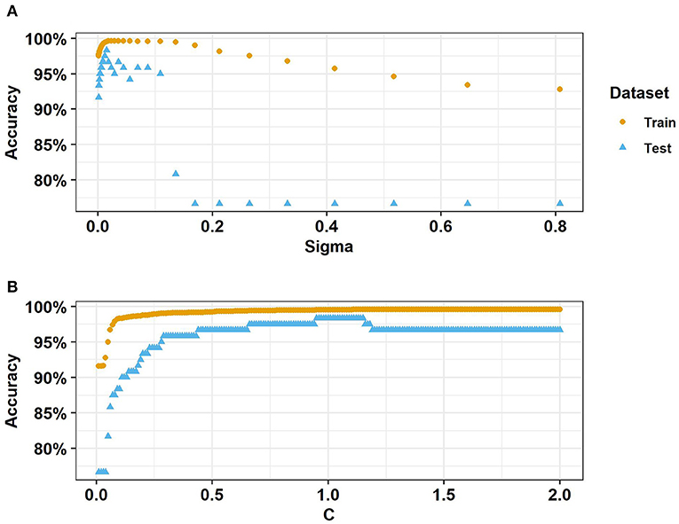
Figure 6. SvmRadial accuracy with (A) sigma ranging from 0.001 to 0.81 with C = 1 and (B) C ranging from 0.01 to 2 with sigma = 0.015. Source: Salveson et al. (Forthcoming). Reprinted with permission. © The Water Research Foundation.
Random forest rule-based model
rfRules is an ensemble classifier based on associative rules (Deng et al., 2014). In the screening, rfRules had the highest event sensitivity at 100% (Table 3). However, it had a testing set accuracy of 54.2% with 55 false positives, which is clearly unacceptable over the 5-day timeframe of the testing set. Replicating with 30 distinct seeds, the testing set accuracy of this model was stochastic, ranging from 54.2 to 98.3% with a median of 82.5%, This indicated the median testing set accuracy was likely better than it appeared in the screening, but more variable compared to ORFsvm. Also, the distribution of testing set accuracies with different seeds was not normally distributed. Based on a paired Wilcoxon test and the same thirty distinct seeds, PCA, rolling median, and differences from the rolling median did not result in a significant increase in testing set accuracy (p > 0.05). However, including both raw data and the differences from the rolling median did increase median testing set accuracy (p = 0.0085), to 93.75%. With that preprocessing, all variables had a varImp importance score of 0 except influent nitrite, settled TOC, influent nitrate difference, raw conductivity, ozone sidestream flow, and influent ammonia difference. With just these six variables, the training time did not meaningfully decrease but the testing set accuracy was significantly higher (p = 0.0046), 94.2% in all 30 seed iterations. rfRules had two tuning parameters: mtry, the number of variables randomly selected for each tree; and maxdepth, the maximum depth of each tree. With the six variables listed above, mtry was varied from one to six and maxdepth was varied from one to five. Training set accuracy generally increased with higher maxdepth and mtry. The maximum testing set accuracy was 94.2%, and this occurred with a maxdepth of at least three and mtry of at least five. This maximum testing set accuracy corresponded to 6 h until the first detection, which would not be competitive with the models described above.
Boosted tree
bstTree is a type of decision tree ensemble in which each subsequent tree is adjusted to optimize performance using a truncated loss function for robustness against outliers (Wang, 2018). In the screening, bstTree had second highest event sensitivity at 89.3% (Table 3) and a testing set accuracy of 95%. However, it had three false positives, which could be considered unacceptable over the 5-day timeframe of the testing set. bstTree testing set accuracy did not depend on seed. None of the investigated preprocessing techniques improved bstTree testing set accuracy. Omitting influent TOC and ozone residual setpoint increased the testing set accuracy to 99.2%. Further omitting variables until only thirteen remained (raw conductivity, influent nitrate, influent conductivity, influent UVT, settled NH4+, settled ORP, settled TOC, biofilter influent total Cl2, biofilter influent pH) resulted in no loss in accuracy and decreased the training time from 32 to 21 s. bstTree had three tuning parameters: maxdepth, the maximum depth of the decision trees; mstop, the number of boosting iterations; and nu, the step size. Maxdepth = 3, mstop = 150, and nu = 0.1 were selected from among the default options based on training set accuracy for the model trainings described above. Ranging maxdepth 1–4, nu from 0.1 to 1, and mstop from 50 to 500 revealed that highest testing set accuracy was achieved with maxdepth = 3 and either nu = 0.1 with mstop = 150 or nu = 1 with any value for mstop. Thus, the default tuning parameters were among the most accurate for bstTree. The testing set accuracy of 99.2% with bstTree was the highest in this study and corresponded to one false negative and zero false positives. The sole false negative occurred on the first datapoint of the event (Figure 7), so this model would have detected the event after about 1 h.
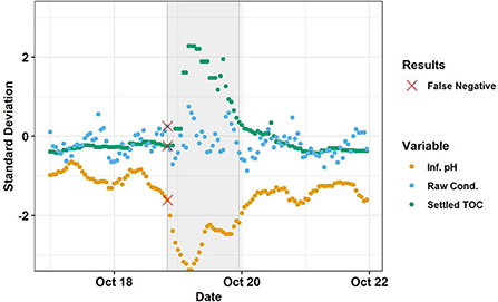
Figure 7. Testing set results of bstTree (n = 0.1, mstop = 150, maxdepth = 3). Trained on the raw data of thirteen variables (raw conductivity, influent nitrate, influent conductivity, influent UVT, settled NH4+, settled ORP, settled TOC, biofilter influent total Cl2, biofilter influent pH). The shaded gray area represents the Event. Red X's indicate false negatives. The three variables whose omission would have resulted in greatest loss in testing set accuracy (influent pH, raw conductivity, and settled TOC), are shown. Source: Salveson et al. (Forthcoming). Reprinted with permission. © The Water Research Foundation.
Actual thresholds
This section shows the time until detection using alert thresholds values that were in place at the SWIFT RC. These alerts were set conservatively lower than corresponding alarms, which were based on ensuring the public health and regulatory compliance. Alerts were in place on six of the variables used in this study (Table 5). Only three were triggered during the testing set event: secondary effluent turbidity, settled water total chlorine, and ozone dose. Secondary effluent turbidity triggered soonest during the event, after just 2 h. However, there were also two alerts for effluent turbidity within the five-day testing set not associated with the industrial event. So, none of these existing alerts would have performed as well as bstTree.
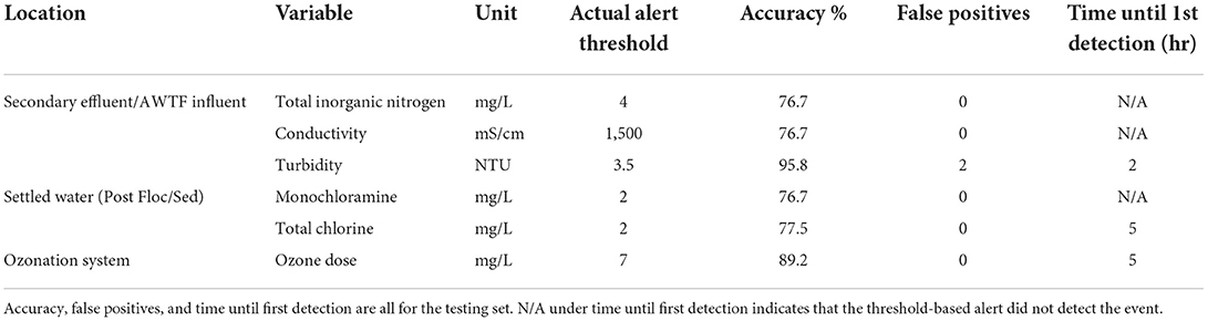
Table 5. Actual threshold-based alerts in place at the AWTF and their performance detecting the event in the testing set.
Data-driven thresholds
Current fixed-threshold-based alerts at the SWIFT RC are based on safety factors, critical control points, and ensuring the public health or regulatory compliance. However, another approach would be to set alert thresholds based on the maximum (or a high percentile) of the data considered normal. This approach could be considered a simple form of SML, in that it would be data-driven, and thresholds could be trained, tested, and refined over time. However, compared to the SML methods described above, this approach would be much simpler since it would be monovariate. In this section, alerts were set based on the maximum or minimum normal datapoint for each variable in the training set. Alerts set this way are herein called “data-driven thresholds.” For pH, UVT, and disinfectant residuals, the data-driven threshold was set to the minimum normal datapoint in the training set (Figure 8). Otherwise, the data-driven threshold was set to the maximum normal datapoint in the training set.

Figure 8. Data-Driven threshold example using influent UVT. The dashed black line represents the threshold. The blue arrow indicates the Normal, training set datapoint on which it was based. Shaded gray areas indicate events. Source: Salveson et al. (Forthcoming). Reprinted with permission. © The Water Research Foundation.
For most variables, a data-driven threshold would not have predicted any datapoints in the testing set where events, so their accuracy was equivalent to the NIR (see Table 6). However, a threshold based influent UVT would have achieved 98.3% testing set accuracy with zero false positives. This testing set accuracy would be equal or better than all of the SML models evaluated except bstTree.

Table 6. Performance of a fixed threshold approach based on each of the 30 variables.
However, greater sample size would be expected to improve the relative performance of the SML models. In contrast, greater sample size might not improve the data-driven threshold results. The use of minima or maxima to set thresholds like was done here would become increasingly conservative (i.e., fewer false positives, more false negatives) with greater sample size because it would allow more time for non-industrial outliers in the Normal training data. This could be counteracted somewhat by setting the threshold based on a specified percentile that strikes the desired balanced between false positives and false negatives.
Discussion
Testing set accuracy has limitations as a performance metric for SML models. For unbalanced data [e.g., data with many more of one class than the other(s)], such as used here, models could achieve over 70% accuracy by always assuming datapoints were Normal, or by randomly guessing Random vs. Event based solely on their proportion in the training set. Furthermore, using only testing set accuracy, the success of models cannot be directly compared across studies, since the accuracy would depend in part on the proportion of classes in the respective datasets.
One alternative metric is balanced accuracy, or what the accuracy would be if there were equal percentages of each class in the dataset. Balanced accuracy is more intercomparable across studies and cannot be increased by increasing the proportion of a specific class. However, in the context of alert systems for the water or wastewater industry, false positives could be a more important error type than false negatives. False positives (i.e., Normal datapoints incorrectly predicted as Event) would waste resources and eventually lead to a boy-who-cried-wolf scenario in which the alert system is disregarded or discontinued. For hourly data frequency, even a 1% false positive rate would lead to false alerts roughly twice per week, which would likely be unacceptable to utility operators. In contrast, many of the datapoints labeled and predicted as an Event in this study could be considered to occur at low levels that would not yet pose an immediate threat to the operation or treatment goals of the facility. Thus, a higher false negative rate could be considered tolerable compared to the acceptable false positive rate. For example, for a dataset with 75% Normal data, a model with 0% false positive rate, 80% false negative rate, and 80% accuracy and 60% balanced accuracy could be considered far preferable to a model with 40% false positive rate, 0% false negative rate, and 70% accuracy and 80% balanced accuracy. Balanced accuracies for the optimized versions of the models selected for in-depth evaluation are shown in Table 4. Except for plr, the optimized versions of all models selected for in-depth evaluation had balanced accuracy over 88%. bstTree had the highest testing set balanced accuracy at 98.2%.
Another alternative performance metric to accuracy is Cohen's Kappa. Cohen's Kappa compares the agreement between the true classifications and the model classifications to the agreement that could occur due to random allocation (Cohen, 1960). The formula for Cohen's Kappa with two classes is:
Where TP is true positives, FP is false positives, FN is false negatives, and TN is true negatives. One of the limitations with Cohen's Kappa is that there is not a universally agreed magnitude considered adequate (i.e., less consensus compared to the typically acceptable p-value threshold of <0.05). One highly cited guideline is that Cohen's Kappa above 0.81 is almost perfect agreement (Landis and Koch, 1977). Except plr, the optimized versions of all models selected for in-depth evaluation exceeded this threshold. bstTree had the highest Cohen's Kappa at 0.976.
Conclusions and future directions
• The model bstTree had the highest testing set accuracy for this dataset, 99.2%. bstTree would have detected the event in about an hour with zero false positives over the 5-day testing set. bstTree also the highest balanced accuracy at 98.2% and Cohen's Kappa at 0.976. Thus, bstTree would have been selected among the SML models investigated in this study for future monitoring and alerts at this site using the studied variables.
• A data-driven fixed threshold based on influent UVT would have resulted in a testing set accuracy of 98.3%, below that of bstTree but only by about 1%.
• The most beneficial preprocessing method differed among the SML model types. Two models performed best without preprocessing, one with PCA, and three with raw data and differences from the rolling median.
• In many cases, some variables could be omitted to decrease training time without loss in accuracy. However, the optimal selection of variables depended on the model.
• Certain SML model types from within the random forest family (e.g., ORFsvm, rfRules) had testing set accuracies that depended on the seed to the random number generator. Thus, the accuracy of these models would be more uncertain in full-scale applications, even with appropriate validation and testing procedures.
Looking to the future, we would make following recommendations:
• As next steps to engineer an accurate, practical, SML-based alert system, we would recommend repeating the above analyses but with greater sample size, including multiple instances of the events in the testing set. This would provide greater confidence about the relative performance of the models, particularly whether the highest-performing model would be best for detecting all events of this type, not just the individual event in this testing set. After that, a small number of high-performing SML models could be piloted in real-time, until an additional event occurs. The time until first detection of the SML models could then be compared in the field against human monitoring and other alert approaches.
• Since Event and Normal datapoints in this dataset were distinguished based on human judgement, the best the models could possibly do would be to match—not exceed—human judgement. On the other hand, a human monitoring the data in real-time might not have concluded that an event was occurring as early as a human evaluating the whole dataset retrospectively. In future research on machine learning for wastewater or reuse alert systems, this could be achieved by simulating industrial discharges in a pilot or flume. Alternatively, real full-scale industrial events could be labeled objectively if the industrial source is known and keeps records of discharge flow (e.g., the landfill that discharges limited quantities of leachate to the WWTP that feeds SWIFT RC) (Gonzalez et al., 2021; Nading et al., 2022).
• A limitation of SML-based alert systems is that they are designed to detect events of a known, previously documented type. If a new type of industrial discharge were to occur associated with different responses from the online instrumentation, this may or may not trigger an SML-based alert. Changes in the water quality pattern at the AWTF during industrial discharge events could also occur due to changes in the treatment operation response at the WWTP. So, a strategic solution would be to employ both SML-based and threshold-based alerts. This would combine the sensitivity of SML with the generalizability of thresholds. These additional thresholds could be set based on training set data, health-based goals, or operational considerations. Advanced multivariate statistical methods for fault or outlier detection other than SML also merit further research in the context of wastewater and reuse (Klanderman et al., 2020).
• While bstTree performed best on the dataset in this study, further research is merited on SML for event detection in other reuse AWTFs and especially for other water quality monitoring contexts. For example, data would generally be noisier in wastewater collection systems, both due to more real variation and more difficulty keeping sensors calibrated. The noisiness of the data can affect which machine learning algorithms perform best (Atla et al., 2011). The length vs. wideness of the dataset can affect, for example, which SML algorithms can be trained quickly (Lindgren et al., 1993; Rännar et al., 1994). So, even in the same AWTF, more sample size—whether in form of more and new variables or more observations collected over time—could change which SML type performs best.
Data availability statement
The original contributions presented in the study are included in the article/Supplementary material. The raw data and R code used in this study are provided in the Supplementary material.
Author contributions
KT: machine learning analysis and first draft of the manuscript. TD, TN, CB, CW, and GS-B: data provision. AB and AS: project management. TD, TN, CB, CW, AB, AS, ED, and GS-B: manuscript revision. ED: concept and design of study. All authors contributed to the article and approved the submitted version.
Acknowledgments
Carollo Engineers, Inc.; the Southern Nevada Water Authority (SNWA); and Jacobs Engineering Group gratefully acknowledge that the Water Research Foundation and the California State Water Board are funders of certain technical information upon which this manuscript is based under Project 5048. Jacobs and SNWA thank the Water Research Foundation and the California State Water Board for their financial, technical, and administrative assistance in funding the project through which this information was discovered.
Conflict of interest
Authors KT, AB, and AS were employed by Carollo Engineers, Inc. Authors TN and TD were employed by Jacobs Engineering Group, Inc.
The remaining authors declare that the research was conducted in the absence of any commercial or financial relationships that could be construed as a potential conflict of interest.
Publisher's note
All claims expressed in this article are solely those of the authors and do not necessarily represent those of their affiliated organizations, or those of the publisher, the editors and the reviewers. Any product that may be evaluated in this article, or claim that may be made by its manufacturer, is not guaranteed or endorsed by the publisher.
Author disclaimer
This material does not necessarily reflect the views and policies of the funders and any mention of trade names or commercial products does not constitute the funders' endorsement or recommendation thereof.
Supplementary material
The Supplementary Material for this article can be found online at: https://www.frontiersin.org/articles/10.3389/frwa.2022.1014556/full#supplementary-material
References
Atla, A., Tada, R., Sheng, V., and Singireddy, N. (2011). Sensitivity of different machine learning algorithms to noise. J. Comput. Sci. Coll. 26, 96–103. doi: 10.5555/1961574.1961594
Clopper, C. J., and Pearson, E. S. (1934). The use of confidence or fiducial limits illustrated in the case of the binomial. Biometrika 26, 404–413. doi: 10.2307/2331986
Cohen, J. (1960). A coefficient of agreement for nominal scales. Educ. Psychol. Meas. 20, 37–46. doi: 10.1177/001316446002000104
Deng, H., Runger, G., Tuv, E., and Bannister, W. (2014). CBC: an associative classifier with a small number of rules. Decis. Support Syst. 59, 163–170. doi: 10.1016/j.dss.2013.11.004
Gonzalez, D., Thompson, K., Quiñones, O., Dickenson, E., and Bott, C. (2021). Granular activated carbon-based treatment and mobility of per- and polyfluoroalkyl substances in potable reuse for aquifer recharge. AWWA Water Sci. 3, e1247. doi: 10.1002/aws2.1247
Hatwell, J., Gaber, M. M., and Muhammad Atif Azad, R. (2021). Gbt-hips: explaining the classifications of gradient boosted tree ensembles. Appl. Sci. 11, 2511. doi: 10.3390/app11062511
Khan, M. A., Shah, M. I., Javed, M. F., Khan, M. I., Rasheed, S., El-Shorbagy, M. A., et al. (2022). Application of random forest for modelling of surface water salinity. Ain Shams Eng. J. 13, 101635. doi: 10.1016/j.asej.2021.11.004
Khan, M. S., and Coulibaly, P. (2006). Application of support vector machine in lake water level prediction. J. Hydrol. Eng. 11, 199–205. doi: 10.1061/(ASCE)1084-0699(2006)11:3(199)
Klanderman, M. C., Newhart, K. B., Cath, T. Y., and Hering, A. S. (2020). Fault isolation for a complex decentralized waste water treatment facility. Appl. Stat. 69, 931–951. doi: 10.1111/rssc.12429
Kuhn, M. (2008). Building predictive models in R using the caret package. J. Stat. Softw. 28, 1–26. doi: 10.18637/jss.v028.i05
Kuhn, M. (2019). The Caret Package, Chapter 6. Github. Available online at: https://topepo.github.io/caret/available-models.html (accessed August 7, 2021).
Landis, J. R., and Koch, G. G. (1977). The measurement of observer agreement for categorical data. Biometrics 33, 159–174. doi: 10.2307/2529310
Lee, S., Kim, J. C., Jung, H. S., Lee, M. J., and Lee, S. (2017). Spatial prediction of flood susceptibility using random-forest and boosted-tree models in Seoul metropolitan city, Korea. Geomatics Nat. Haz. Risk 8, 1185–1203. doi: 10.1080/19475705.2017.1308971
Lee, S., Lee, C.-W., and Kim, J.-C. (2019). “Groundwater productivity potential mapping using logistic regression and boosted tree models: the case of Okcheon city in Korea,” in Advances in Remote Sensing and Geo Informatics Applications, eds H. M. El-Askary, S. Lee, E. Heggy, and B. Pradhan (Cham: Springer), 321–327. doi: 10.1007/978-3-030-01440-7_69
Lin, S., Novitski, L. N., Qi, J., and Stevenson, R. J. (2018). Landsat TM/ETM+ and machine-learning algorithms for limnological studies and algal bloom management of inland lakes. J. Appl. Remote Sens. 12, 026003. doi: 10.1117/1.JRS.12.026003
Lindgren, F., Geladi, P., and Wold, S. (1993). The kernel algorithm for PLS. J. Chemom. 7, 45–59. doi: 10.1002/cem.1180070104
Matsumoto, M., and Nishimura, T. (1998). Mersenne twister: a 623-dimensionally equidistributed uniform pseudo-random number generator. ACM Trans. Model. Comput. Simul. 8, 3–30. doi: 10.1145/272991.272995
Menze, B. H., Kelm, B. M., Splitthoff, D. N., Koethe, U., and Hamprecht, F. A. (2011). “On oblique random forests,” in Machine Learning and Knowledge Discovery in Databases, eds D. Gunopulos, T. Hofmann, D. Malerba, and M. Vazirgiannis (Athens: Springer), 453–469. doi: 10.1007/978-3-642-23783-6_29
Nading, T., Dickenson, E., Salveson, A., Branch, A., and Schimmoller, L. (2022). An Enhanced Source Control Framework for Industrial Contaminants in Potable Reuse. Alexandria, VA: The Water Research Foundation.
Nolan, J. R. (2002). Computer systems that learn: an empirical study of the effect of noise on the performance of three classification methods. Exp. Syst. Appl. 23, 39–47. doi: 10.1016/S0957-4174(02)00026-X
Park, M. Y., and Hastie, T. (2008). Penalized logistic regression for detecting gene interactions. Biostatistics 9, 30–50. doi: 10.1093/biostatistics/kxm010
Peng, J., Chen, C., Zhou, M., Xiaohua, X., Zhou, Y., and Luo, C. (2020). A machine-learning approach to forecast aggravation risk in patients with acute exacerbation of chronic obstructive pulmonary disease with clinical indicators. Sci. Rep. 10, 3118. doi: 10.1038/s41598-020-60042-1
Poona, N., van Niekerk, A., and Ismail, R. (2016). Investigating the utility of oblique tree-based ensembles for the classification of hyperspectral data. Sensors. 16, 1918. doi: 10.3390/s16111918
Rännar, S., Lindgren, F., Geladi, P., and Wold, S. (1994). A PLS kernel algorithm for data sets with many variables and fewer objects. Part 1: theory and algorithm. J. Chemom. 8, 111–125. doi: 10.1002/cem.1180080204
Rodriguez, J. J., Kuncheva, L. I., and Alonso, C. J. (2006). Rotation forest: a new classifier ensemble method. IEEE Trans. Pattern Anal. Mach. Intell. 28, 1619–1630. doi: 10.1109/TPAMI.2006.211
Salveson, A., Branch, A., Thompson, K., Weeks, B., Mansell, S., Nading, T., et al (Forthcoming). Integrating Real-Time Collection System Monitoring Approaches into Enhanced Source Control Programs for Potable Reuse. Project 5048. Denver, CO: The Water Research Foundation.
Schölkopf, B., Sung, K. K., Burges, C. J. C., Girosi, F., Niyogi, P., Poggio, T., et al. (1997). Comparing support vector machines with gaussian kernels to radial basis function classifiers. IEEE Trans. Sig. Process. 45, 2758–2765. doi: 10.1109/78.650102
Suykens, J. A. K., and Hornegger, J. (1999). Least squares support vector machine classifiers. Neural Process. Lett. 9, 293–300. doi: 10.1023/A:1018628609742
SWRCB (2021). DPR Framework 2nd Edition Addendum—Early Draft of Anticipated Criteria for Direct Potable Reuse. Sacramento, CA: California Water Boards.
Tan, G., Yan, J., Gao, C., and Yang, S. (2012). Prediction of water quality time series data based on least squares support vector machine. Proc. Eng. 31, 1194–1199. doi: 10.1016/j.proeng.2012.01.1162
Thompson, K. A., and Dickenson, E. R. V. (2021). Using machine learning classification to detect simulated increases of de facto reuse and urban stormwater surges in surface water. Water Res. 204, 117556. doi: 10.1016/j.watres.2021.117556
Wang, F., Wang, Y., Zhang, K., Hu, M., Weng, Q., and Zhang, H. (2021). Spatial heterogeneity modeling of water quality based on random forest regression and model interpretation. Environ. Res. 202, 111660. doi: 10.1016/j.envres.2021.111660
Keywords: machine learning, potable reuse, random forest, source control, artificial neural network, data preprocessing
Citation: Thompson KA, Branch A, Nading T, Dziura T, Salazar-Benites G, Wilson C, Bott C, Salveson A and Dickenson ERV (2022) Detecting industrial discharges at an advanced water reuse facility using online instrumentation and supervised machine learning binary classification. Front. Water 4:1014556. doi: 10.3389/frwa.2022.1014556
Received: 08 August 2022; Accepted: 30 September 2022;
Published: 04 November 2022.
Edited by:
Ali Saber, University of Toronto, CanadaReviewed by:
Fabio Di Nunno, University of Cassino, ItalyAlex Neumann, University of Toronto Scarborough, Canada
Copyright © 2022 Thompson, Branch, Nading, Dziura, Salazar-Benites, Wilson, Bott, Salveson and Dickenson. This is an open-access article distributed under the terms of the Creative Commons Attribution License (CC BY). The use, distribution or reproduction in other forums is permitted, provided the original author(s) and the copyright owner(s) are credited and that the original publication in this journal is cited, in accordance with accepted academic practice. No use, distribution or reproduction is permitted which does not comply with these terms.
*Correspondence: Kyle A. Thompson, kthompson@carollo.com