 Arianna Valmassoi1,2*
 Jan D. Keller3
- 1Hans-Ertel-Centre for Weather Research, Climate Monitoring and Diagnostics, Bonn, Germany
- 2Institute of Geosciences, University of Bonn, Bonn, Germany
- 3Deutscher Wetterdienst, Offenbach, Germany
Irrigation is the process of artificially providing water to agricultural lands in order to provide crops with the necessary water supply to ensure or foster the growth of the plants. However, its implications reach beyond the agro-economic aspect as irrigation affects the soil-land-atmosphere interactions and thus influences the water and energy cycles in the Earth system. Past studies have shown how through these interactions, an increase in soil moisture due to irrigation also affects the atmospheric state and its dynamics. Thus, the lack of representation of irrigation in numerical Earth system models—be it for reanalysis, weather forecasting or climate prediction—can lead to significant errors and biases in various parameters of the system including but not limited to surface temperature and precipitation. In this study, we aim to summarize and discuss currently available irrigation parameterizations across different numerical models. This provides a reference framework to understand the impact of irrigation on the various components of Earth system models. Specifically, we discuss the impact of these parameterizations in the context of their spatio-temporal scale representation and point out the benefits and limitations of the various approaches. In fact, most of the parameterizations use irrigation as a direct modification of soil moisture with just a few implementations add irrigation as a form of surface water. While the former method might be suitable for coarse spatio-temporal scales, the latter better resembles the range of employed irrigation techniques. From the analysis, we find that not only the method or the spatio-temporal scales but the actual amount of water used is of great importance to the response of the Earth system model.
1. Introduction
Agricultural production is becoming crucial not only for the economy but also for food security. In fact, with a growing world population, food demand is also rising while at the same time, changes in the hydrological cycle and climate affect both agricultural yield and species sustainability (IPCC, 2014; Chatzopoulos et al., 2019; Zampieri et al., 2019). For the past decades, irrigation has become important in sustaining the food production. While only 20% of the cultivated land is irrigated, it accounts for about 40% of the total food production (Bin Abdullah, 2006; Siebert and Döll, 2010; Sridhar, 2013). Furthermore, irrigation enables an increased food security especially in regions which would not otherwise allow for crop growth due to adverse climate conditions, such as very arid areas (Sridhar, 2013). However, agricultural water scarcity is already affecting 39% of the global cropland areas and that this is bound to increase in the next decades (Liu et al., 2022).
Agriculture is also one of the three main activities driving natural land conversion (Luyssaert et al., 2014; McDermid et al., 2017). In this respect, land cover changes have only recently been highlighted as an important factor in the climate system as described by Mahmood et al. (2014). They further highlight how not only land use conversion but also its management can cause considerable impacts on the Earth system with irrigation being the practice with the largest bio-geophysical effect on climate. Sometimes the effect of the managements changes has the same impact that the changes in land cover do (Jia et al., 2019).
Irrigation generally refers to the agriculture practices of watering plants. Although irrigation earliest records date back to the Classical Greek and Imperial Roman periods, archaeological works date it back to 5000 BC (Angelakιs et al., 2020). Despite irrigation being present and crucial throughout the centuries, the vast expansion of its use was a non-linear process string in the early 1800s. This development included the interaction not only within the entrepreneurial sector but also with engineering and public administration (Angelakιs et al., 2020). To date, the irrigation techniques used across the world vary depending on the climate conditions and historical context, aside than from the funding available. Despite the very different conditions, the irrigation techniques can be grouped into four categories (i.e., surface, sprinkler, micro, and subirrigation), depending on how the water is delivered to the plants (see Section 2.1).
Aside from increasing the agricultural yield and food security, irrigation is a land management practice that is often accompanied by permanent and irreversible land transformations (Angelakιs et al., 2020). This is caused by both the modification of the land to adapt for both agricultural use and the distribution networks and the water and salt balances changes (Squatriti, 1998). Further, irrigation increases the soil water available to the plants. This, in turn, impacts the soil-atmosphere feedback, as soil moisture is an inland water source for the atmosphere through evapotranspiration (Seneviratne et al., 2010). The land evapotranspiration is also a major component of the water cycle, thus influencing not only the energetic surface balance, but also the atmospheric processes themselves.
While irrigation has been used throughout the millennia, its effect on the climate system has only been addressed in recent decades, the reason being the complexity of the involved feedback processes within the Earth system and the lack of related data and tools. The ongoing improvement in the observational networks and systems, both in quantity and quality (i.e., spatial resolution), and the advancements of numerical models opened up promising perspective in investigating the impact of the irrigation management on the Earth system.
The first observational studies on the impact of irrigation on the Earth system can be dated back to the 1953 with the study by Chudnowskii, referred by de Vries (1959) when a theoretical framework for the energy balance and the near-surface is presented. Later on, Budyko (1972) highlights irrigation as an important modification to the evapotranspiration, as evidence from observations showed. The first modeling studies referring to irrigation can be found in Milly and Dunne (1994). While their study focuses on the sensitivity of the water cycle to the capacity of the land to hold water, they argue that the results can be interpreted also as a anthropogenic modification of the water cycle, intended as irrigation. The first modeling studies explicitly addressing irrigation are regional works by Lohar and Pal (1995) for India first, and then by De Ridder and Gallée (1998) for Israel and Segal et al. (1998) for the Contiguous United States. The first global studies about irrigation were published some years later, e.g., Boucher et al. (2004). While most of the observational studies argue how irrigation modifies the evapotranspiration (de Vries, 1959; Flohn, 1963), the first modeling studies include both irrigation as a modification of the soil moisture (Lohar and Pal, 1995; De Ridder and Gallée, 1998) and as a evaporation modification (Segal et al., 1998; Boucher et al., 2004; Evans and Zaitchik, 2008). Most of the studies involved with designing an irrigation parameterization follow the work by Kueppers et al. (2007) and their concept of irrigation as soil moisture modification, despite Lobell et al. (2006a) using it first and highlighting how it was mentioned only as an extreme scenario. Lobell et al. (2006a,b) opened up the topic of irrigation at the global scales and showed how its relevance in the context of a changing climate. Lobell et al. (2008) and later Cook et al. (2011) demonstrated how the irrigation signal did mask the increase in temperatures due to climate change at multiple food baskets across the world, after seeing it for California in a previous study (Bonfils and Lobell, 2007). Sacks et al. (2009) was the first study that attempted to include irrigation water as a rational of several drivers, and limit its amount, which was identified as the key aspect in both comparisons and applicability to the reality. However, the core mathematical representation of irrigation developed by Ozdogan et al. (2009) follows Kueppers et al. (2007), and not Boucher et al. (2004), and further defines irrigation as driven by the soil moisture availability. Leng et al. (2013) developed one of the most used irrigation parameterizations after Ozdogan et al. (2009), affirming irrigation as a physical modification of the soil moisture. This scheme is widely used also in follow-up regional and high resolution studies across the globe, irrespective of the irrigation time-scales and techniques. This parameterization by Leng et al. (2013) is further implemented to close the water cycle by adding the irrigation water extraction (Leng et al., 2014, 2017). Only later with Leng et al. (2017) and Valmassoi et al. (2020a), the irrigation water is not seen as a direct modification of the soil moisture, but includes a physical representation of the process, e.g., the interaction of the irrigation with the canopy. While the importance of the irrigation volume used in the simulation is highlighted since Sacks et al. (2009), only Decker et al. (2017) demonstrates the pitfalls of using offline irrigation computations to force simulations and the importance of having high-resolutions.
In this review, we first define irrigation in the Earth system (cf. Section 2), presenting both its techniques divided by the main delivery methods (cf. Section 2.1) and the impact found in previous studies (cf. Section 2.2). Then the existing irrigation parameterizations (ct. Section 3) are described, categorized based on the activation method (ct. Section 3.1) and the variables that are directly affected (cf. Section 3.3) by the estimated irrigation water (cf. Section 3.2). In Section 4, we discuss the relation of the irrigation parameterizations to the actual techniques either through the process representation (cf Section 4.1) or via the relevant spatio-temporal scales (cf Section 4.2), highlighting some relevant physical considerations (cf Section 4.3). In Section 5.1, we provide an overview of the irrigation water amount applied in the available studies including both the focus region and the period considered. Finally, we point out future research perspectives in this field (cf Section 6), and provide a summary and the main conclusions in Section 7.
2. Irrigation in the earth system
2.1. Irrigation techniques
In modern agriculture, there are several irrigation techniques that have been developed to meet specific crop/regional needs. Originally, the irrigation techniques are grouped into three main systems [Brouwer et al. (1985a,b), a major reference for irrigation in agriculture] namely surface, drip and sprinkler. More recent sources that attempt to generalize irrigation techniques across the world tend to group them into four main delivery methods, and call the “drip” technique “micro” (Phocaides, 2000; Bjorneberg, 2013; Irmak, 2018). The four methods can be represented with the conceptualization of Figure 1 and are defined, as general and as specific as possible, as follows:
1. Surface (A): the water is delivered to the field through hydrants and it is either spread over the whole area (furrow/basin irrigation) or from its borders (border irrigation) (Brouwer et al., 1985b; Phocaides, 2000).
2. Sprinkler: the water is delivered as raindrops that precipitate over the agricultural area. There are several variations of this method, and for this purpose, we highlight that they can depend on the height (over/under the foliage, respectively B/C and A) and diameter of the application, and rate (Phocaides, 2000; Bjorneberg, 2013).
3. Micro: the so-called “localized” irrigation, where the water is delivered directly around a limited soil surface around the plants. Further, the water is applied at a low rate and pressure. However, this method is mainly employed in permanently installed systems, e.g., trees, vineyards (Bjorneberg, 2013).
4. Subirrigation (D): in this method, the water is applied to change the water table height (Bjorneberg, 2013), and it has a high potential for areas with a high degree of drainage requirements (Irmak, 2018). This method is generally used in the horticultural industry in greenhouses and nursery plant productions (Irmak, 2018). However, it is not used in arid or semi-arid areas, as irrigation water is needed for the crop germination (Bjorneberg, 2013).
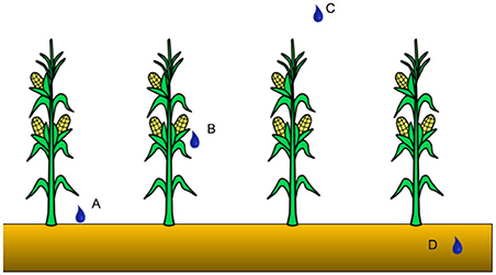
Figure 1. Irrigation water delivery method conceptualization in the modeling perspective, figure adapted from Valmassoi et al. (2020a). Process A can represent the surface irrigation and the micro, depending on the spatial extent and amount of water used, as well as the sprinkler applied only below the foliage. Process B and C can both represent the sprinkler depending how high above the canopy the sprinkler water is applied. Process D instead reflects the subirrigation. For an in-depth discussion refer to Section 4.3.
While the description seems generic, the wide geographical variability and its constant evolution over time makes very complicated to give a general definition.
The Food and Agriculture Organization (FAO) provides six training manuals for irrigation (e.g., Brouwer et al., 1985a,b, Manual 1 and 5), which are still considered the starting point for addressing irrigation in general. For specific modern information on the techniques and the recommended configurations, the base reference should be Phocaides (2000), Bjorneberg (2013), Irmak (2018), and Brouwer et al. (1985b).
2.2. Irrigation impact on the Earth system
As mentioned in the introduction, the importance of irrigation goes beyond the agricultural aspect as it affects the soil moisture, which in turn has a crucial role in the context of surface energy and water balance (Seneviratne et al., 2010). Irrigation land management practices have been recognized as a crucial component of the anthropogenic impact on the climate (Sacks et al., 2009; Luyssaert et al., 2014; Thiery et al., 2020), but was included only in the most recent Intergovernmental Panel on Climate Change (IPCC) 5th Assessment Report (AR5) (Jia et al., 2019; Thiery et al., 2020). Furthermore, irrigation has to be considered as a major unaccounted anthropogenic source of water vapor (Boucher et al., 2004), and accounts for intra- and inter-basin water extraction and redistribution. While the impact of irrigation on the local climate can be detected in in-situ observations and remote sensing products, numerical models can also be utilized to understand more complex feedback effects as well as their implications for the Earth system as a whole.
The goal of irrigation is to increase water available for crops and, thus, sustain them throughout the growing season. Therefore, a major effect is an increase in the soil moisture content. In absence of precipitation, this can be used as a basis for detection algorithms, e.g., developed by Lawston et al. (2017), Brocca et al. (2018), or Zaussinger et al. (2019). Such an increase in soil moisture by irrigation is also observed in many modeling studies (e.g., Boucher et al., 2004; Kueppers et al., 2007; Sacks et al., 2009; Puma and Cook, 2010; Thiery et al., 2017; Valmassoi et al., 2020b). There is very high confidence (Jia et al., 2019) that a higher soil moisture content affects the surface energy partitioning by increasing the upward moisture flux and decreasing the sensible heat flux (Thiery et al., 2017; Valmassoi et al., 2020c). The associated change in the Bowen ratio causes the widely observed surface cooling effect of irrigation (e.g., Lobell et al., 2006a, 2009; Kueppers et al., 2007; Puma and Cook, 2010; Sorooshian et al., 2011; Thiery et al., 2017; Valmassoi et al., 2020a; Nie et al., 2021), and the increase in the near-surface atmospheric moisture (Mahmood et al., 2008). While the global annual cooling of 1.3 K described in Lobell et al. (2006a) seems somewhat high, Boucher et al. (2004) and Thiery et al. (2017) provide estimates that look more realistic with 0.05 and 0.20 K, respectively. Further, all studies shows that the cooling has a strong regional component. The decrease in the diurnal maximum temperatures can go from 3 to 8 K (de Rosnay, 2003; Douglas et al., 2009; Saeed et al., 2009; Guimberteau et al., 2012; Tuinenburg et al., 2014). The high variability is both due to regional signals but can be caused by the overestimation of the cooling effect in global studies, i.e., up to 4.9 times higher in the Indo-Gangetic Plain of India in the global study by Thiery et al. (2020) as compared to simulations with realistic water volumes and high resolution simulations (Jha et al., 2022).
Regional studies are often used to further investigate the signals of irrigation and provide deeper insights to the involved processes and their effects. Such studies mostly focus on larger, highly irrigated areas such as India (e.g., de Rosnay, 2003; Douglas et al., 2009; Saeed et al., 2009; Guimberteau et al., 2012; Tuinenburg et al., 2014), the North China Plain (e.g., Leng et al., 2015; Kang and Eltahir, 2018; Wu et al., 2018), or the Contiguous United States (e.g., Pei et al., 2016; Lu et al., 2017) as well as smaller areas like California (e.g., Kueppers et al., 2007; Sorooshian et al., 2011; Yang et al., 2017), or parts of Italy (e.g., Valmassoi et al., 2020a; Dari et al., 2021). Most studies show a strong diurnal cycle of the expected irrigation-induced cooling effect where the diurnal maximum temperature is impacted most while the minimum seems not to be affected (e.g., Kueppers et al., 2007; Jia et al., 2019). This pronounced diurnal cycle is also reflected in the boundary layer structure, where several studies observed a lowering of the boundary layer height due to the combined decrease of the temperature and increase of the water vapor (e.g., Pielke et al., 2007; Mahmood et al., 2008; Valmassoi et al., 2020c).
With respect to effects on atmospheric circulations, the spatial heterogeneity of the irrigated areas is reflected in the horizontal discontinuity of the affected fluxes as well as local circulation changes (e.g., Barnston and Schickedanz, 1984; Pielke and Zeng, 1989; Kueppers et al., 2007; Aegerter et al., 2017). The changes in thermodynamic air mass properties and circulation are found to potentially affect precipitation locally and/or downwind, due to water vapor transport (e.g., Bonfils and Lobell, 2007; Deangelis et al., 2010; Wei et al., 2013) and/or the change in stability (Valmassoi et al., 2020b). These regional changes are found to affect the large scale synoptic circulations, such as the weakening and the delaying of the Indian Monsoon (e.g., Douglas et al., 2009; Saeed et al., 2009; Lee and Ngan, 2011; Guimberteau et al., 2012) or the change in the remote precipitation patterns over the Sahel region (e.g., Wei et al., 2013; Im and Eltahir, 2014).
While there is a regional component of the irrigation impact on the Earth system, Sacks et al. (2009) and Wada et al. (2013) identify the irrigation representation in models and the water amount used as crucial causes of the associated uncertainties, such as the regional signals.
3. Existing irrigation parameterizations
In order to represent the irrigation process and its effects as realistically as possible in the modeling of the Earth system, parametrizations of this process have been developed. In the following, we present the main equations of the various parameterization approaches albeit with a harmonized notation.
First, we will discuss the topic of irrigation activation which is crucial due to the anthropogenic nature of the process. Here, timing generally refers to the decision to activate the irrigation parameterization. There are mainly three approaches to determine when irrigation is initialized, namely, the usage of (i) geographical invariant spatial fields, (ii) the time of the day, (iii) physical time-varying thresholds, or a combination of any of these.
Then, we will detail the existing parameterization approaches. These can be divided into four groups distinguished by the model quantity that is directly affected by the irrigation (i.e., where the irrigation water is applied to), and, thus, where direct impacts on the model's governing equations arise. Irrigation can be represented as (i) a change in soil moisture, (ii) water applied at the surface, (iii) a water vapor source, and (iv) a modification to the model rain water.
3.1. Irrigation activation
In this section, we present the approaches used to activate irrigation parameterizations. We distinguish between the approaches of using (i) spatial information, (ii) temporal constraints and (iii) physical thresholds.
3.1.1. Spatial dimension
In this approach, geographical fields are used as time invariant information to determine the initialization of irrigation, and these includes (i) the area equipped for irrigation, (ii) the vegetation state data set, and (iii) the crop-types. In reality, these parameters are subject to changes from 1 year to the next, since climatic conditions and weather patterns may change. Also other parameters may vary due to the anthropogenic nature of irrigation, e.g., crop types could be rotated, the area equipped for irrigation can be altered (e.g., Puma and Cook, 2010; Brown and Pervez, 2014). However, for numerical models these information are commonly kept constant across the years albeit for a fixed monthly cycle. A summary of the available dataset at the time is given in Table 1.
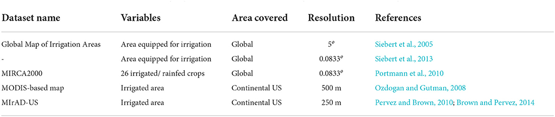
Table 1. Table that summarize the available geographical dataset about area irrigated or equipped for irrigation.
Most of the studies include the spatial information on irrigation through the area equipped for irrigation map (Döll and Siebert, 2002; Siebert et al., 2005, 2013) from the FAO AQUASTAT database (e.g., Bonfils and Lobell, 2007; Sacks et al., 2009; Saeed et al., 2009; Leng et al., 2013; Lu et al., 2015; Valmassoi et al., 2020a). This is a global gridded dataset that combines the national level census data of agricultural water usage for areas equipped for irrigation, giving the percentage of the irrigated land within a grid cell. The first of these dataset had a spatial resolution of 5o (Siebert et al., 2005), with the newest at a 0.0833o resolution (around 9 km at mid-latitudes, Siebert et al., 2013). While Siebert and Döll (2010) provide the area equipped for irrigation, Portmann et al. (2010) made the MIRCA2000 dataset of monthly distribution fields of the irrigation/rainfed agricultural area available, divided in 26 classes also at a spatial resolution of 0.0833o representative for the time period 1998–2002. The dataset further includes spatial information about multi-cropping agricultural land as well as irrigation calendars. MIRCA2000 has been used in multiple studies, e.g., Leng et al. (2017), Cheng et al. (2021), and Liu et al. (2021). For the continental United States, two other datasets of irrigated areas are available at higher resolution, namely (i) Ozdogan and Gutman (2008) at ~500 meters resolution and (ii) the Irrigated Agriculture Dataset (MIrAD-US) developed by Pervez and Brown (2010) and Brown and Pervez (2014) at 250 meters. Both datasets are based on MODIS measurements and agricultural census maps. While the former combines also climatological indexes and supervised decision-based classification algorithm, the latter uses only vegetation considerations as well as county-level census data. MIrAD-US also provides temporal information on changes of irrigated land and is updated every 5 years (Brown and Pervez, 2014). While the dataset of Ozdogan and Gutman (2008) has been used by Ozdogan et al. (2009), Leng et al. (2013), Qian et al. (2013), and Harding et al. (2015), MIrAD-US was employed in, e.g., Pei et al. (2016). While the previously mentioned dataset have been widely used across modeling studies, it is worth to mention that they are not the only ones, e.g., Salmon et al. (2015). However, such datasets have currently not been used for modeling studies.
The MIRCA2000 dataset can be used not only to derive the area irrigated, but it provides information about the crops cultivated in the reference year 2000. Lobell et al. (2009) extended the FAO area equipped for irrigation dataset by a plant functional type (PFT) for irrigated crops. The new PFT fraction is subtracted to the original value to ensure a consistent total agricultural area with the control simulation. While the method proposed by Lobell et al. (2009) does not modify any of the plant properties, Leng et al. (2017) added the crop type information to the Community Land Model (CLM, v4.5). These data can be used to determine the area fraction within a grid cell that is of a specific crop-type and whether it is irrigated or not. Irrigation can then be applied only to the irrigated portion of the grid cell fraction on which crops are grown. If there is a residual in the crop partitioning within each grid cell, it is considered as an unmanaged crop and it is treated as a C3-type of grass. Another way to include specific vegetation properties is by including irrigated crops specific vegetation parameters, which have a low roughness length, low stomatal resistance, leaf area similar to grassland and forest, and albedo similar to deciduous broad-leaf trees. This has been done by Kueppers et al. (2007) in their study using the RegCM3 numerical model (Seth et al., 2007).
Aside from using the vegetation and its parameters as constant in time, it can be used to regulate irrigation as well. For example, the Leaf Area Index (LAI) or the greenness fraction (GF) can be used to determine if the plant growing season has started or ended. These spatial data are usually an invariant geographical field with an annual cycle.
This means that the season begins and ends when 40% of the annual range (GFmax − GFmin) is reached, which allows to include areas with very different growing season in the same simulation.
3.1.2. Temporal constraint
A popular approach to activate the irrigation parameterization is to employ temporal constraints. Within this framework, a specific hour of the day is chosen to activate the irrigation (e.g., Adegoke et al., 2003; Leng et al., 2013; Valmassoi et al., 2020a). This time can be used to either set a model prognostic variable to a target value, e.g., Adegoke et al. (2003) where soil moisture is set to saturation at 00UTC, or to combine it with a duration in hours. The latter approach is expressed as the number of consecutive hours hI, and is used to localize the irrigation procedure in time (e.g., Leng et al., 2013; Valmassoi et al., 2020a). Examples of different start hours and length are 06 local and 4 h (e.g., Ozdogan et al., 2009; Leng et al., 2013; Yang et al., 2016), 08 (Liu et al., 2021) or 09 (Evans and Zaitchik, 2008; Wu et al., 2018) local time and for 2 h and 30 min, respectively, or a sensitivity to these parameters by Valmassoi et al. (2020a). The irrigation duration period is usually employed to equally partition the calculated water over all the consecutive hours, transforming the quantity to a rate (mms−1), for example. Only in Pei et al. (2016) the 2 h duration is used to apply irrigation at a specified rate, whenever the soil moisture threshold is met.
With the described approaches, the temporal constrains are applied each day throughout the whole simulation period, and irrigation is only ended in combination with other thresholds. For example, Valmassoi et al. (2020a) include an arbitrary beginning and end of irrigation, indicated in terms of Julian days. Further, irrigation does not need to be applied each day despite a potential plant water stress. For example, Evans and Zaitchik (2008) and Valmassoi et al. (2020a) apply irrigation once every 7 days, and every 7, 3 and 1 days, respectively. This deviating timing enables the parameterization to allow for a more flexible and more realistic approach.
3.1.3. Physical threshold
The previously mentioned irrigation thresholds do not explicitly account for the plant water stress. However, this characteristic is crucial and would contribute to a more realistic representation of the irrigation process. In general, plants do not suffer water stress when the soil moisture falls below field capacity1, because the roots are able to partly extract the water bound by the soil matrix, so there is Ready Available Water (RAW) for the plants. The lower limit of the extraction is the wilting point (θwp), at which water is so strongly bound to the soil matrix that the roots are not able to extract it. The amount of water that the soil can hold (and plants can extract) between the field capacity and the wilting point is the Total Available Water (TAW). The ratio between RAW and TAW is defined as the depletion fraction (p), which depends on crop type and soil type. Given this definition, p can be used to determine when the plant suffers water stress and thus relates to a specific soil moisture value, called critical soil moisture (θc):
Values of p can largely vary depending on the plant type and need to be corrected for high evapotranspiration regimes (Brouwer et al., 1985b) 5 mm/d. However, a value of p = 0.5 is commonly used for many crops (Brouwer et al., 1985b). Manabe et al. (1965) and Seneviratne et al. (2010) use higher values of p, namely, 0.5 to 0.8 and 0.75, respectively, with high rise vegetation being included (e.g., conifer trees p = 0.7). This concept has been implemented using the (i) βt function (Oleson et al., 2013, p.169) and (ii) a soil moisture index (Seneviratne et al., 2010), SMI. The former is the result of a weighted average of the plant wilting factor and the fraction of roots for all considered layers (Oleson et al., 2013) p.169. In general, the plant is suffering stress if βt is less than 1 (e.g., Leng et al., 2013; Lu et al., 2015), with 0 being the asymptotic value leading to the permanent wilting point. For the soil moisture index, no root density information is needed. Ozdogan et al. (2009) introduced the Soil Moisture Availability threshold (SMA, θat) defined as:
which leads to a different formulation of θc and p. This allows for a tuning of the SMA to a specific case study, instead of using crop and soil types, whose dataset have a coarse resolution (e.g., MIRCA2000 Table 1). In literature, the following SMA thresholds are used: 0.5 by Ozdogan et al. (2009) and Qian et al. (2013), 0.2 by Pei et al. (2014) and Pei et al. (2016), 0.1 by Lawston et al. (2015)2, 0.6 by Yang et al. (2016)3, and 0.47–0.5 and 0.45, 0.5–0.6, as well as 0.55 and 0.48 by Sorooshian et al. (2011), Liu et al. (2021), and Wu et al. (2018)4, respectively. The thresholds are evaluated for different soil layers in the studies: Pei et al. (2016) evaluate it against the second soil layer (10–40 cm), Ozdogan et al. (2009), Sorooshian et al. (2011), Yang et al. (2016), and Lawston et al. (2015) use the root-zone levels, and Wu et al. (2018) and Liu et al. (2021) apply the thresholds to the weighted average of the first two soil layers.
It should be mentioned that Decker et al. (2017) apply a variation of Equation (3), and instead of the field capacity, they use the saturation soil moisture (θs). There, threshold value θat = 0.5 has to be met in all the layers in the root-zone.
The wide range of possible SMA threshold values leads to the inclusion of regimes that could be already considered water stress for some crops (Brouwer et al., 1985b). The target soil moisture value is aimed to prevent plant water stress within the modeling framework. Therefore, Leng et al. (2013) formulates the new threshold5 as the weighted average of the critical soil moisture and the saturation one for each soil layer as:
where θs, i is the i-th layer soil moisture saturation. The Firr is used as a weighting factor, between 0 and 1, to determine the relevance of the two thresholds. At the limits, the scheme's assumption falls back to the saturation soil moisture (Firr = 1) and Firr = 0 at the other limit when plants start experiencing water stress.
Other physical thresholds have been mentioned in literature but without further justification, such as not activating irrigation (i) when the soil temperature is below 12oC (arbitrarily defined by Kueppers et al., 2008), (ii) during large solar radiation flux periods, i.e., solar radiation less than 50Wm−2 (arbitrarily defined by Sorooshian et al., 2011), (iii) until the first 10 cm soil temperature exceed 5oC in the previous 24 h, (iv) until the daily mean 2-meter temperature is above 8oC (Pei et al., 2016).
3.2. Irrigation water calculation
As highlighted in multiple studies, the amount of irrigation water applied plays a crucial role in the impact. Depending on the threshold and timing definition, the methods found can be grouped into (i) a-priori estimation and (ii) driven by the soil conditions.
3.2.1. A-priori irrigation water amount
Several studies use estimates provided by local, national or international entities given as annual accumulated volumes. Examples from existing studies for the sources include but are not limited to the Kansas Geological Survey (Pei et al., 2016), the United States Geological Survey (USGS) water use report and province-level data for China from the China State Statistical Bureau (Sacks et al., 2009), or Eurostat (European Union) irrigation water amount reports (Valmassoi et al., 2020a). Other authors use irrigation water amount reconstructions, which are created combining irrigation maps and offline models, e.g., Cook et al. (2015) with the dataset by Wisser et al. (2010). These reconstructed amounts are provided as irrigation rates.
In general, these data are transferred onto an irrigation depth (mm · m−2 · y−1) by assuming that irrigation takes place in a certain fraction of the area, e.g., the area equipped for irrigation. More specifically, Valmassoi et al. (2020a) assume that the annual amount is applied only over the summer crop season, thus, deriving an irrigation depth in mmd−1 (VI), which is expressed as irrigation water rate (WI, in mms−1) as:
where hI is the aforementioned number of consecutive hours and TI the number of days between one irrigation application and the next, in contrast to most other studies, where irrigation is applied every day (TI = 1).
Overall, studies report various irrigation rates for different regions. A summary of these are presented in Table 2.
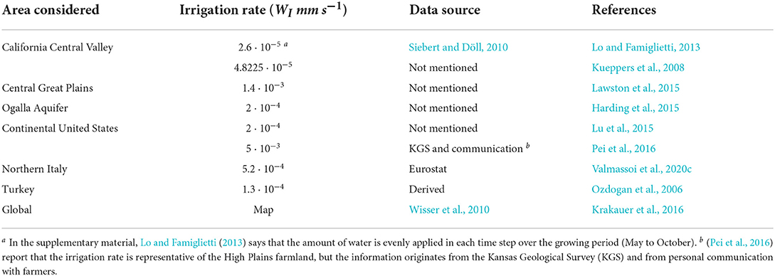
Table 2. Table of reported irrigation rates (WI) of various studies using an a-priori volume/rate.
The irrigation rate values span across two orders of magnitude over an area that covers the continental United States or parts of it. It should be noted that some studies cover the same region but for sometimes very different periods, from different decades or multi-year data sets to short high-resolution simulations for only a few days. Ozdogan et al. (2006) mention that their irrigation rate is derived in a way to keep the soil moisture at saturation, but it is neither mentioned how it is calculated nor where the water is applied to. This approach can include the interannual variability of the water used for irrigation, however most of the studies use the amount from a reference year. The Wisser et al. (2010) map can be used to integrate the temporal resolution of the irrigation water amount, but that is done only in the studies employing the simulations by Cook et al. (2015). A reason could be in the limitations of offline irrigation water estimations, discussed later in Section 5.1.
3.2.2. Soil-driven irrigation water amount
As previously seen, physical constraints can be used to initiate irrigation, and from those the necessary water amount can be calculated starting from the water available to the plants (θa). While Marcella and Eltahir (2014) propose a method that accounts for explicitly including the porosity in the computation, others rely on the threshold definition itself:
where θi has to be calculated only for the liquid water content to already account for the plant-available water. The maximum function is used in Leng et al. (2013), but not by e.g., Decker et al. (2017), Wu et al. (2018), and Liu et al. (2021). This implies that Leng et al. (2013) does not allow for a surplus in one layer to reduce the deficit in another. The different studies also apply different Z-values to determine how many soil-layers are considered: Leng et al. (2013) and Decker et al. (2017) use all the layers between the surface and the root-zone, while e.g., Wu et al. (2018) and Liu et al. (2021) only use the first two layers. The drip method by Evans and Zaitchik (2008) calculates the irrigation water amount as the difference between the evapotranspiration without and with plant water stress, which includes all root-zone layers.
This water calculation allows to investigate the interannual volumes used and potentially compare them with the estimates available.
3.3. Application of irrigation water
Here, we group the existing parameterizations by the model quantity that is directly altered after the conceptualization of Figure 1. Understanding where the irrigation water is applied within a numerical model allows to identify the directly affected processes in the Earth system, as well as the efficiency of the technique. From the literature, irrigation has been assumed to affect directly (i) soil moisture at different levels, (ii) precipitation at the surface, (iii) the rain water mixing ratio and the (iv) water vapor flux.
3.3.1. Irrigation as soil moisture
Most of the available parameterizations see irrigation as a direct modification to the soil moisture, but they use different assumptions regarding the parameters. Table 3 groups the parameterizations by the soil moisture quantity they relate to, the reference value to trigger it and the part of the soil column affected. In the following, we describe the parameterizations and their parameters in more detail.
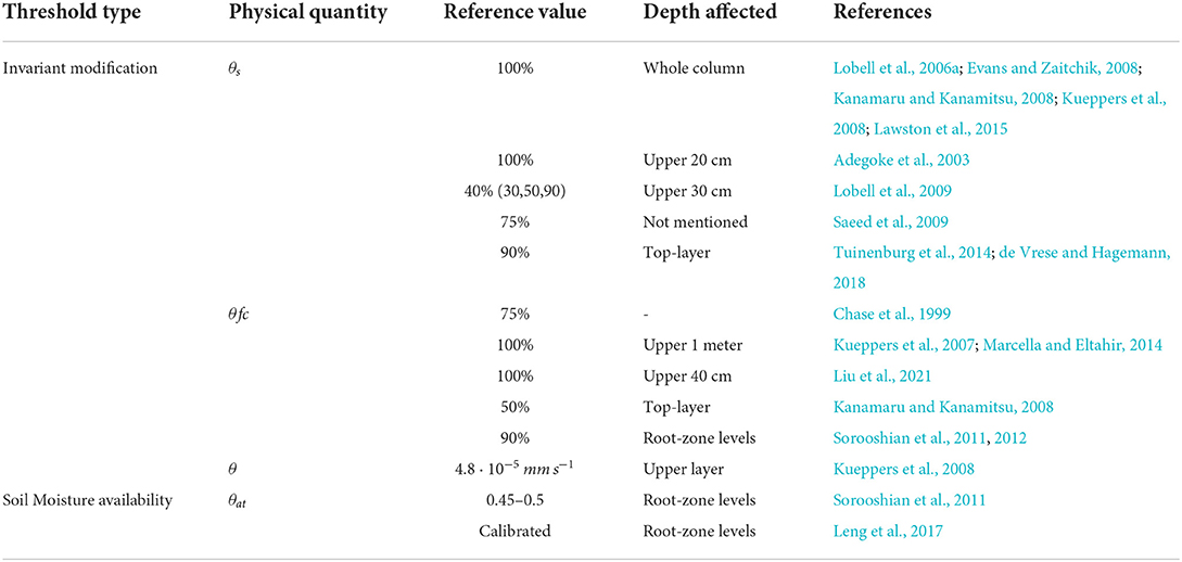
Table 3. Summary of parameterizations with irrigation implemented as soil moisture modification.
First of all, we highlight how the view of irrigation as direct soil moisture modification (Process D of Figure 1) is widely spread among past as well as recent studies, from Chase et al. (1999) to Leng et al. (2017). This representation type is used with a wide variety of parameters, affected soil levels as well as several activation threshold usages. The latter is now used to group a more in depth presentation of the studies.
Several studies that investigate irrigation parameterizations in atmospheric numerical models, represent irrigation as an invariant modification on some of the physical model variables with some studies using the aforementioned activation thresholds, such as timing, to reset these variables. The most common approach is to set the soil moisture field to a predefined reference value, e.g., the saturation level (θs), the field capacity (θfc), or a fraction of them. In this context, the saturation level approach implies usually much wetter conditions than the soil at field capacity, since the former includes filling the pores. However, this water is strongly bound and not really available to the plants. While some studies do not limit the depth of the impact of the irrigation (e.g., Lobell et al., 2006a), others hypothesize that only the upper layers are affected, such as the upper 20–40 cm (e.g., Adegoke et al., 2003; Lobell et al., 2009; Liu et al., 2021), the first meter (Kueppers et al., 2007), or the layers that include the plant roots (Sorooshian et al., 2011; Leng et al., 2017). For soil saturation, the available studies use very different threshold values, from 100% in Lobell et al. (2006a), Kanamaru and Kanamitsu (2008), Kueppers et al. (2008), Evans and Zaitchik (2008), and Lawston et al. (2015), to 90% for Tuinenburg et al. (2014) and their follow-up studies, 75% for Saeed et al. (2009), and down to 40% for Lobell et al. (2009). Lobell et al. (2006a) and the follow-up work of Lobell et al. (2009) provide a useful set of sensitivity experiments with different saturation thresholds and different depths affected. In both of their all soil columns defined as cropland within the Community Atmospheric Model v.3 (CAM3) are affected throughout the whole simulation. Lobell et al. (2006a) meant to represent irrigation with the soil saturated only as a sensitivity experiment, and the follow-up determined the threshold of 40% based on the examination of the soil moisture in their control experiment (Lobell et al., 2009). There, the monthly averaged values were below that threshold for the whole local summer season, and above for the remainder of the year. For completeness, sensitivity tests with different thresholds were performed for the arbitrary values of 30%, 50% and 90%, where the latter was considered an extreme value. Despite the considerations by Lobell et al. (2006a), that same approach was used by Kueppers et al. (2008) for the Regional Spectral Model (RSM). In a follow up study, Kanamaru and Kanamitsu (2008) argue that the previously prescribed soil moisture in RSM was too high. Therefore, they set top soil layer at field capacity as the highest irrigation scenario. Saeed et al. (2009) justify the choice affirming that irrigation practices are assumed to fulfill optimal conditions for the crops, in order to “transpire at a potential rate.” As reasoning, the authors refer to a highly simplified vegetation stomata regulation. We therefore assume that the potential rate refers to the evapotranspiration observed under no soil water stresses (Brouwer et al., 1985b).
Instead of saturating the soil moisture, some studies use the field capacity as it is the upper limit of the plant available water (Kirkham, 2005). While most of the studies here correct the soil moisture for the whole simulation, Chase et al. (1999) uses this value as the initial condition for the simulation. As in the previous threshold, also here the studies use multiple threshold values, from 100 to 50%. The studies that set the soil moisture at field capacity differ both in the depth affected, the root-zone levels (upper 1 m) or the upmost 40 cm, and in the conservation of the water applied. While Kueppers et al. (2007) and Liu et al. (2021) just set the new soil moisture value, Marcella and Eltahir (2014) allow to both conserve the water balance of the column and to return the water needed for irrigation as a diagnostic. Few studies use threshold values as fraction of the field capacity, e.g., 50% Kanamaru and Kanamitsu (2008) or 90% for Sorooshian et al. (2012). Sorooshian et al. (2012) use Kueppers et al. (2007), Kanamaru and Kanamitsu (2008) and Haddeland et al. (2006) to justify the threshold choice. However, Kueppers et al. (2007) do not use any threshold and Haddeland et al. (2006) only mention that irrigation starts when the evapotranspiration is limited by the soil moisture. While the threshold for water stress depends on the crop type and stage, Brouwer et al. (1985b) suggests that for general crops it is half the total available water, which is a function of the difference between the field capacity and the wilting point.
Another method used in literature to continuously affect the soil moisture is used by Kueppers et al. (2008) in the Davis Regional Climate Model (DRCM). There, the authors add the water to the surface soil moisture at a uniform rate of 4.8225 · 10−5mms−1 for all the time steps in the simulations.
Studies that employ this soil moisture availability threshold type do not necessarily apply the irrigation water to reset the soil moisture to the threshold value. Sorooshian et al. (2011) use it only to trigger irrigation and the soil moisture is increased using the determined irrigation rates until it reaches the field capacity. On the other hand, Leng et al. (2017) apply the irrigation water amount calculated from Equation (6) to all root-zone soil layers directly. There the threshold level for the irrigation is calculated using Equation (4), and a Firr parameter is used to tune the parameterization for each administrative region within the domain by employing the Siebert and Döll (2010) irrigation water use map.
3.3.2. Irrigation as water applied at the surface
When irrigation is applied as water at the surface, the main difference between the parameterizatrions lies in the derivation of the amount used, aside from the thresholds employed. As can be observed from Table 4, the parameterizations are also differentiated by their impact on the canopy water balance.
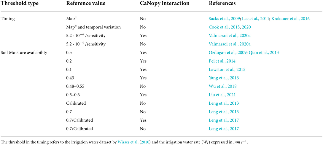
Table 4. Summary of the irrigation parameterizations as water applied to the surface with the different parameters used in the available studies.
The differentiation is mentioned because some numerical models do not include a canopy water balance equation in their land surface scheme, e.g., WRF's Rapid Update Cycle (RUC) (Smirnova et al., 2016), or the Terra Land Surface model used in both COSMO and ICON models (Schättler et al., 2018). Therefore, it is important to differentiate irrigation application that interact with the canopy or not, given the availability of canopy water balance schemes in the numerical models.
Table 4 highlights how the parameterizations that apply the water at the surface can be divided in two different threshold types, i.e., based on the timing and the soil moisture availability.
The first threshold uses a-priori water estimations for the application, either coming from the Wisser et al. (2010) dataset or county-based estimates. Sacks et al. (2009), Cook et al. (2015, 2020), and Krakauer et al. (2016) also added the a-priori irrigation values as rain-rates albeit bypassing the canopy interception. The map used by Sacks et al. (2009), and thus by Lee et al. (2011), to determine the irrigation amount is invariant in their simulation, while Cook et al. (2015, 2020) and Krakauer et al. (2016) use the same reconstructed irrigation rate from Wisser et al. (2010), but for the periods 1901–2002 and 2000, respectively. Valmassoi et al. (2020a) instead use estimates coming from the Eurostat census data (Eurostat, 2013), and the sensitivity is performed by changing the number of consecutive hours (hI) with the daily amount being kept constant.
The soil moisture availability threshold comes from either (i) Equation (3) (Ozdogan et al., 2009) or (ii) Equation (4) from Leng et al. (2013). In the studies that follow Ozdogan et al. (2009) the irrigation water is applied above the canopy (e.g., Pei et al., 2014; Yang et al., 2016), and only Wu et al. (2018) apply it without canopy interaction. The reason lies in their affirmation that the irrigation water is included as effective precipitation6, which does not include the interception.
For the soil moisture threshold defined initially by Leng et al. (2013) (cf. Equation 4), the water is applied directly at the surface after the canopy interception. In a later work, Leng et al. (2017) add two other ways to include the irrigation water: (i) directly on the canopy and (ii) on the ground surface. Similarly, also Valmassoi et al. (2020a) provides two different parameterizations called drip and channel depending if the water interacts with the canopy or not, respectively. In both parameterizations' sets, the irrigation water (WI) is added to the precipitation model field. In the case of Leng et al. (2017) irrigation applied at the surface, the amount is also scaled by a specific period to allow for a quick pouring on the ground.
3.3.3. Irrigation as atmospheric rain water
Previous studies mentioned that the application of the irrigation water to the precipitation field takes place at the canopy, which does not account for the droplets evaporation or drift loss in the atmosphere. We are currently not aware of any other than the “sprinkler” scheme by Valmassoi et al. (2020a) that includes these processes to which the irrigation water can be exposed. To account for possible microphysical processes, the irrigation water has to be added to the rain water mixing ratio as:
where ρk is the air density in the kth-layer of Δzk thickness. The rain rate is modified only in the lowest mass-layer, so it is assumed that the sprinkler water does not directly reach beyond the first model layer. In their study, Valmassoi et al. (2020a) set the height of such level to 20 meters.
While studies such as Ozdogan et al. (2009) uses the same name (“sprinkler”) for their representation, they never include a direct atmospheric interaction with the irrigation droplets.
3.3.4. Irrigation as water vapor source
The inclusion of irrigation as a water vapor source reflects the theoretical considerations made by de Vries (1959) and Flohn (1963) in investigating the impact of irrigation on the climate system. This approach has been used by only two studies: Boucher et al. (2004) and Evans and Zaitchik (2008).
Boucher et al. (2004) derives the irrigation as a water vapor flux spatial field combining two dataset: the annual net evapotranspiration from irrigation derived from a scenario approach at country level and the area equipped for irrigation (Döll and Siebert, 2002). They included this information in five methods of increasing complexity, with the first four taken as sensitivity experiments, and the fifth being used in a numerical climate experiment. In the sensitivity experiments, irrigation is represented as additional water vapor in the atmosphere with different horizontal and vertical distributions. For the climate simulation, Boucher et al. (2004) prescribe an artificial surface water vapor source equal to the irrigation flux determined from the spatial data. This additional water flux enters in the energy balance as an evaporative cooling term in the surface energy budget of the model, independently from the meteorological conditions.
Evans and Zaitchik (2008) instead modify the canopy resistance, thus directly affecting the plant evapotranspiration calculation. While this is not clearly stated in the study, the irrigation water is not applied in the form of liquid water (e.g., precipitation, soil moisture) as the soil moisture values are similar to the control simulation.
3.4. Accounting for irrigation through data assimilation
When irrigation is not represented in a physical model, an alternative way to include the effect of irrigation in the model state is to apply a data assimilation approach. Here, the analysis increments to the soil moisture content do not only represent the forecast deviations of precipitation and evaporation but also account for the errors due to the lack of irrigation processes. This mechanism has been indicated by Tuinenburg and de Vries (2017) for the ERA-Interim reanalysis, in which the soil moisture analysis increments are linked to irrigation patterns. As irrigation is not directly observed by measurements providing spatial coverage, efforts are focusing on correcting the soil moisture with respect to the irrigation-related effects. A possible approach is to assimilate GRACE satellite data (e.g., Girotto et al., 2017) which has the total column water as a residual of the main gravimetric measurements. Nie et al. (2019) provide a more thorough study comparing assimilated soil moisture and an irrigation parameterization and their respective effect on groundwater storage representation. While this is a relatively new field, it is a promising approach to either account for the missing water redistribution due to human action or as a tool to identify model shortcomings related to irrigation.
3.5. Irrigation water source
Most of the previously presented irrigation schemes do introduce the irrigation water (WI) ad hoc in the numerical model, due to the uncertainties related to water extraction and model limitations. Only Leng et al. (2014), and later Leng et al. (2017), include the irrigation water extraction within the numerical scheme. Leng et al. (2014) use the USGS census data, and later the Siebert and Döll (2010) dataset, for water withdrawal to define the ratio of irrigated water extracted from surface water (fsrf) and groundwater (fgrd) with respect to the total amount. To allow for different sources of water withdrawal, the respective water storage (Ssrc) is updated for every irrigated grid point by subtracting water amount (WI) weighing its ratio:
where src can stand for either groundwater (grd) or surface sources (srf). For the groundwater extraction, Leng et al. (2017) update the water table with the weighted irrigation water extraction (WI · fsrc) divided by the soil yield (Sy). Further, the weighted irrigation extraction is included also in the water stored in the unconfined aquifer below the lowest model level and the total groundwater storage (Leng et al., 2014).
The extraction scheme allows also for non-local water extraction, within the same basin (g), in case the surface water requirement cannot be met locally. This is done by updating (Equation 8), for Ssrf, as:
To determine the new extraction in the n non-irrigated grid points in the g-basin, only if Equation (8) for the surface sources is negative, as:
If the is not sufficient to satisfy the requirements, the water is assumed to come from other sources, e.g., inter-basin, but the actual method is not specified.
4. Representation of irrigation in models
When anthropogenic processes such as irrigation are included in a numerical model, a complex requirement is to have representation that is suitable and generic enough. We discuss this issue from three perspectives. First, the process representation itself, which is not always clear and straight-forward for some of the existing irrigation parameterizations with regard to how these relate to the actual irrigation techniques as described in Section 2.1. Second, scale representation plays an important role. As irrigation impacts the soil moisture, the soil moisture variations can span across multiple spatial and temporal scales, from the order of one meter to 106 km and 1 min to more than a decade, respectively (Seneviratne et al., 2010). Third, physical considerations with respect to the interaction of soil moisture content, plants and irrigation.
4.1. Process representation
When comparing the available parameterizations regarding their irrigation delivery method, one distinctive characteristic is the variable to which the irrigation water WI is applied to. Figure 1 provides a conceptualization of the delivery methods from the modeling perspective, which shows where in the model domain the water could be applied with respect to the plant canopy.
In micro-irrigation (cf. Section 2.1) the application of water is within the diameter of the canopy, i.e., in the order of meters. However, numerical models have grid sizes that are larger by at least two orders of magnitude and can, thus, not realistically represent this process.
While the temporal scales of irrigation can also not be represented explicitly, the quick water release associated with surface irrigation can be emulated by scaling the water amount with a specific time, as shown in Section 3.3.2 by Leng et al. (2017). When the temporal aspect of the water release is not considered, the surface and the sprinkler delivery methods, that apply the water below the foliage, can be both interpreted as water introduced below the crop canopy or directly onto the surface (Figure 1, Process A). In this case, the irrigation techniques can be represented with the parameterizations in Section 3.3.2 that do not include the canopy interception.
When sprinkler water is injected above the plant foliage, it could be implemented either by process B or C in Figure 1 depending on the distance between the delivery system and the canopy. If the water is applied close to the foliage (process B), water loss might be minimal with respect to wind or droplet evaporation effects (Bjorneberg, 2013). If the distance is larger, droplet evaporation and wind advection become relevant, such that the water is subject to rain water micro-physical atmospheric processes (Figure 1, Process C) as described in Section 3.3.3. It could similarly be seen as an atmospheric water source (Section 3.3.4) as atmospheric water vapor is directly affected.
For the subirrigation delivery method (Figure 1, Process D), a water table height change is induced. Specifically, the water table is brought to the surface level or the vertical location of the saturated area within the soil is altered as described by the parameterizations in Section 3.3.1. However, it should be noted that for several crop types a saturated soil can cause issues for the plants' health (Bradley et al., 2017). The consequence of too much water in and over the soil could, thus, result in severe losses. This holds even for rice fields, which are tolerant to flood/water excess but suffer the consequences of anaerobic environment conditions (Panda and Barik, 2021). Furthermore, a lowering of the water table through effective drainage can overall improve the crop-yield (Gramlich et al., 2018; Manik et al., 2019).
4.2. Scale considerations
From the previous section consideration, it is clear that the parameterization relation to the actual delivery method depends on the scales considered.
The sprinkler delivery methods discussed above relate to different vertical atmospheric scales. Further, the upward water distribution through irrigation depends also on the lower atmospheric model layer thickness. This was introduced by Boucher et al. (2004), where they argue that the modification of the atmospheric moisture content by the direct effect of irrigation was intended as a sensitivity experiment. As sprinklers are not able to spray the water very far from the surface, models with very thick atmospheric layers near the surface, might not be able to realistically include the vertical water dispersion that would be observed. Thus, a suitable vertical model resolution might be needed to restrict the direct vertical influence of the sprinkler delivery method on the atmosphere (Figure 1, Process C). While the maximum heights of water dispersion from sprinklers vary greatly on the specifics of the system itself (Phocaides, 2000), modern efficient low-pressure systems with center-pivot and moving systems reach heights of 1–3 meters and 2–4 meters above the soil, respectively (Bjorneberg, 2013). A layer thickness at the surface of these scales is not practical for a numerical model above horizontal resolutions of a kilometer, due to the stability of the numeric solutions. However, the lowest atmospheric model thickness can be increase to a more suitable value if the model timestep is included in the consideration. In fact, the sprinkler irrigation water can be advected upward by the atmospheric turbulence directly, if the integration time is long enough.
However, for large enough horizontal resolutions the sprinkler delivery method could be parameterized also with the surface water application above the canopy of Section 3.3.2 (Figure 1, Process B), as the direct horizontal diffusion can be neglected. If the timestep of the modeling setting is further increased, then the infiltration of the irrigation water from the surface to the underneath soil layers can take place within the same timestep. Thus, the soil-moisture increase due to irrigation happens instantaneously from the land-atmosphere coupling perspective, thus, leading to irrigation directly affecting soil moisture (cf. Section 3.3.1).
Another scale consideration has to be made regarding the canopy water balance impact on the irrigation application. The timestep length has to be suitable with the modeling7 and climate conditions to properly capture irrigation entering the canopy water balance. For example, during dry conditions the permanence of water on the leaves is very low, thus the model timestep has to be tuned to correctly capture its temporal variability. The scale considerations are another possible reason of the lack of irrigation-specific delivery method in global coarse resolution studies, aside from the absence of adequate global or regional maps. However, the actual representation becomes important when the spatio-temporal resolution of the models are increased to better represent other land and/or atmospheric processes, e.g., convection.
4.3. Physical considerations
As previously mentioned, the soil moisture content regulates the evapotranspiration regimes accordingly to the limitation factors (Seneviratne et al., 2010). Soil moisture values below the critical value (θc) lead to plants regulating the evapotranspiration depending on the available soil water, leading to a soil moisture limited regime. On the other hand, when the soil moisture content is above the critical value, the incoming energy is limiting the evapotranspiration, and therefore the surface energy partitioning (Seneviratne et al., 2010).
The evapotranspiration regime impacts the actual response of the atmospheric system when irrigation increases the soil moisture above the critical value. This is addressed by Lobell et al. (2009), with the usage of the sensitivity simulations of irrigation as different percentages of the saturated soil moisture value (30,40,50,90). They highlight that simulated air temperatures are almost identical for the experiments, which means that the modeled evapotranspiration fluxes are insensitive to soil moisture increases above 30% of their saturation levels. The 30% threshold is lower than the commonly assumed p-value of 0.5 for the crops (see Equation 2 in Section 3.1.3, Brouwer et al., 1985b). In their model version, the equation governing soil evaporation saturates between 20 and 30% of the soil saturation, depending on the texture (Lobell et al., 2009). In addition, the plant transpiration accounts for one-third of the evapotranspiration flux and it is similarly insensitive to soil moisture levels above 30% above the saturation value. Lobell et al. (2009) further discuss how the frequency of irrigation rather than the threshold level can determine the impact on the atmosphere. While the threshold might not directly impact the atmospheric variables, it is, however, crucial to determine the water amount as it is relevant for Earth system water balances and sustainability considerations.
5. Uncertainties and limitations
5.1. Irrigation water amount
This section provides an overview of the uncertainties and limitations regarding the irrigation water amount of the various studies. The irrigation water amount also provides an independent validation dataset for parameterizations that do not prescribe it.
Table 5 lists irrigation rates from the aforementioned parameterizations (cf. Table 3) as well as other sources. We group the focus areas using the series of reference regions of the IPCC Special Report on Managing the Risks of Extreme Events and Disasters to Advance Climate Adaptation (SREX, van Oldenborgh et al., 2014) to the sub-regions for clarity. Table 5 highlights two main problems that come up in comparing and/or assessing irrigation in numerical models from past studies: (i) not all studies report the applied irrigation amount and (ii) the reported values vary across several orders' magnitude for the same regions. The lack of reporting (also mentioned in Sacks et al., 2009) interferes with an appropriate comparison of studies using different numerical models and/or spatio-temporal scales, which in turn increases the uncertainties related to the irrigation impact on the Earth system. Even when irrigation information is reported, it might not be possible to convert it to values comparable to other studies.
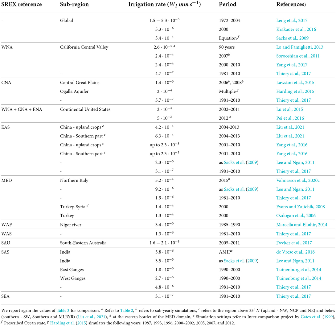
Table 5. Table with the irrigation rates (WI) of the different studies including the derived amounts from the available studies.
The studies where we were able to determine an irrigation rate show very different values, not only globally, but also for the same region of the world. While, there is the temporal increase of irrigation amount observed by Puma and Cook (2010), the reporting of the simulated period is given to provide context. For example, Sacks et al. (2009) used prescribed ocean states and a 30-years simulation, and since the dataset for building the irrigation maps were taken around the year 2000, we assume their simulations are representative of that year. This makes the estimates of the irrigation rates of Sacks et al. (2009) comparable with the ones from Krakauer et al. (2016), which are two order magnitude lower. While the two studies use the same period, they do not use the same model or irrigation rate. Therefore, we cannot draw sustained conclusions about the large differences of the surface cooling effects over irrigated areas (0.061 and 0.665 K, respectively).
It is even more difficult to compare studies that cover the same region but for different periods. However, depending on the geographical area, the irrigation water use might not have changed drastically over time (Puma and Cook, 2010). The situation is easier if there is an overlap, such as for SAS, WNA or EAS. In those cases, Table 5 still shows an irrigation rate variability as high as four orders' magnitude. For example, the difference observed for EAS would lead to a minimum irrigation water amount difference of about 34mm · d−1, considering the rates from Yang et al. (2016) and Liu et al. (2021). Similarly, WNA irrigation rate differences lead to a minimum diurnal difference of about 20mm · d−1, which is higher than the maximum value of 3.4mm · d−1 that is the diurnal accumulated precipitation in the upwind side of the Sierra Nevada (Yang et al., 2017). Furthermore, differences in the irrigation volumes can be explained when considering both the model grid resolution and the spatial distribution of the irrigated area. In fact, coarse model resolution is not able to capture the high spatial variability that leads to very different irrigation volumes driven by the climate conditions (Decker et al., 2017).
While some authors use the available irrigation reconstructions or estimates to calibrate their model or as input (e.g., Tuinenburg et al., 2014; Krakauer et al., 2016; Pei et al., 2016; Leng et al., 2017) use them for comparison. Pei et al. (2016) find biases in the heavily irrigated areas in their study, which is just in part due to the discrepancies of the irrigation fraction map when compared to the used MODIS irrigated croplands. However, the main source of the differences is ascribed to the assumptions in the irrigation scheme, intended as the irrigation rate and duration (see Section 3.3.3), which is not representative for other regions and/or irrigation techniques. Tuinenburg et al. (2014) find that differences in irrigation water amount with respect to the reference Siebert and Döll (2010) varies a lot depending on the model used, from 5 to 89% for the same season (MAM). This leads to a diurnal difference of water applied of a similar magnitude of the diurnal average precipitation for most of the models (Tuinenburg et al., 2014).
To summarize, the uncertainties related to the irrigation amount thus can be ascribed to their assumptions in the calculation. In the literature there are three different ways to obtain the irrigation water amount: (i) fixed value, (ii) online derivation and (iii) offline derivation. While there is no current best practice, we highlight the main limitations of each method so that past and future works' irrigation impact on climate can be contextualized. The fixed amount seems the best solution when the volumes come from a reliable source, and it includes less than optimal irrigation volumes, which are commonly used in real world applications (Siebert and Döll, 2010). However, this might not be applicable for areas and/or region with data scarcity, or it can lead to representativity issues in multi-year simulations. In this case, a good solution is to derive the irrigation water amount within each timestep. However, such approach could lead to unrealistic water amounts due to the model biases themselves. Even in the absence of model biases, the water needed is a function of the soil characteristics, i.e., soil types and parameters, or agricultural practices, which are not well represented. The online computation of water requirements opens up the possibility to include a validation or comparison of the obtained results to available census data, and a discussion about the volumes obtained with the offline derived dataset. The offline dataset provides an interesting model output with a consistent spatial and temporal representation, which seems suitable to be used as forcing for a earth system simulation. However, these datasets exhibit several limitations as, first and foremost, they do not account for the feedback effect that irrigation has on the atmosphere, which is the reason of including explicitly the irrigation parameterizations in the Earth system models. Wisser et al. (2008) show that the combined uncertainty of crop management and weather conditions can lead to water estimations uncertainties of 30% circa, with the weather variability having a strong regional component leading up to ±70% variability. Similar results are found by Decker et al. (2017), where they obtained a 25% increase in irrigation water when using offline model for south eastern Australia (Decker et al., 2017). This problem could be partially resolved if only observational datasets are used to force the model, so that the crop-water demand is affected by the effect of irrigation on the atmosphere. However, observational datasets are generally not dense enough, which can cause an increase of irrigation water demand due to the lack of small-scales representation, as shown by Decker et al. (2017) in a modeling approach.
5.2. Irrigation water extraction
While the irrigation water amount used in the simulations is crucial for any consideration and/or comparison between the studies available in literature, its source for extraction provides several uncertainties. Similarly to the actual irrigation volumes used, also the source type and location is difficult to determine. First of all, irrigation water is either pumped from the groundwater or taken from surface sources, such as rivers, lakes or dams (Döll et al., 2012; Wada et al., 2014).
While irrigation water generally comes from either surface and groundwater sources, it is a well-know problem that pipes or channels are used to transport the water to the fields. From the modeling perspective this means that the sources might not be located near-enough to be considered in the same grid-point, needing an internal water redistribution, aside from the inclusion of the water loss from the pipes to the Earth system. Leng et al. (2017) propose a water extraction scheme based on the water extraction dataset (cf Section 3.5), which allows also for using nearby grid-point in the same basin. While such approach provides a suitable theoretical base, it can be applied safely only to coarse model resolutions due to the importance of drainage direction in actual irrigation practices (Brouwer et al., 1985b) and the usage of open air irrigation channels (Moghazi and Ismail, 1997; Kimaro et al., 2019).
5.3. Model limitations
The limitations in representing irrigation in Earth system models does not lie only in the possible physical representations discussed before. In fact, the model representation of the Earth system processes themselves affect the complexity of the irrigation parameterizations.
Section 3.3.2 already introduced this concept when differentiating the representation of irrigation as water applied at the surface. There, the possibility of irrigation water interacting with the plant leaves could depend on the availability of a canopy water balance scheme in the model itself. The model parameterizations can influence not only that, but also the possibility of including water extraction methods mentioned in the previous section, thus closing the water balance. Numerical weather prediction models in particular might not have a dynamic river routing system and/or a groundwater table, e.g., ICON, WRF-ARW with Noah land surface model (Skamarock et al., 2008; Schättler et al., 2018).
Further, models with static land use and cover maps are not going to be able to capture the crop rotations performed and the interaction between irrigation, land parameters and climate, which has been showed to have a strong impact depending on the region considered (McDermid et al., 2017). Singh et al. (2018) show how the crop cover management, and not only irrigation, can affect the land-atmosphere coupling as the agriculture mid-latitude areas lies in the energetic transitional regimes.
6. Research perspectives
Despite the advances in existing literature, several open research questions still exist. For instance, there is large confidence about a cooling effect of irrigation (cf. AR5) but the magnitude of this effect is still not certain neither at the local nor at the global scales. Further, there is a lot of variability among the studies with respect to the irrigation water amount and its parameterization, especially in Earth system modeling approaches. Another open issue is the low confidence on the impact of irrigation on precipitation. While the ongoing increase in resolution of the models is helping to better understand this feedback, the inclusion of specific irrigation parameterizations prevents the replication of similar schemes with small differences in the parameters and/or the thresholds' choices.
Therefore, there is a strong need for a more coordinated and consistent implementations of irrigation parameterizations in order to assess model and process uncertainties together with better observational datasets. This would also support developments for numerous applications that range from impact modeling to numerical weather prediction and seasonal to sub-seasonal forecasting, to more consistent reanalyzes products and integrated impact assessment for other sectors (e.g., agriculture).
6.1. Consistency across models and regions
The inclusion of irrigation in Earth system models does not always reflect a consistent and realistic process representation and/or adequate spatio-temporal scales considerations (see Section 4). Especially with respect to the initialization of irrigation, the variety of threshold and/or target values leads to a large variation of irrigation water amounts applied in the different models (see Section 5.1). The approach toward more consistent implementations should already start at the differences in the energy partitioning (e.g., Sacks et al., 2009; Krakauer et al., 2016). Further, it is crucial for the precipitation feedback due to the convection representation issues in models (Prein et al., 2021). Therefore, a shift in paradigm would be prudent, from developing a multitude of parameterizations to synthesizing available schemes in a process- and scale-based approach consistent across the available models. New parameterizations and studies should always have a clear reasoning for their irrigation water amount estimates as well as well-motivated threshold choices. Currently, only the Weather Research and Forecasting (WRF-ARW), the Community Land Model (CLM) and the NASA GISS8 include explicitly irrigation, the first two as a parameterization and the latter as a forcing. There is no known plans to include irrigation in other models than ICON-LAM, in the DETECT project 9. Further, there is a need to properly include the water extraction from the soil in order to close the water budget, which is currently available only in CLM.
In addition, Figure 2 shows how several irrigated regions, such as Western Asia (WAS), Sahara (SAH), Western Africa (WAF) or Southern-East Asia (SEA), are currently not included significantly in literature probably due to their small extent, the lack of available data or a low fraction of irrigated area.
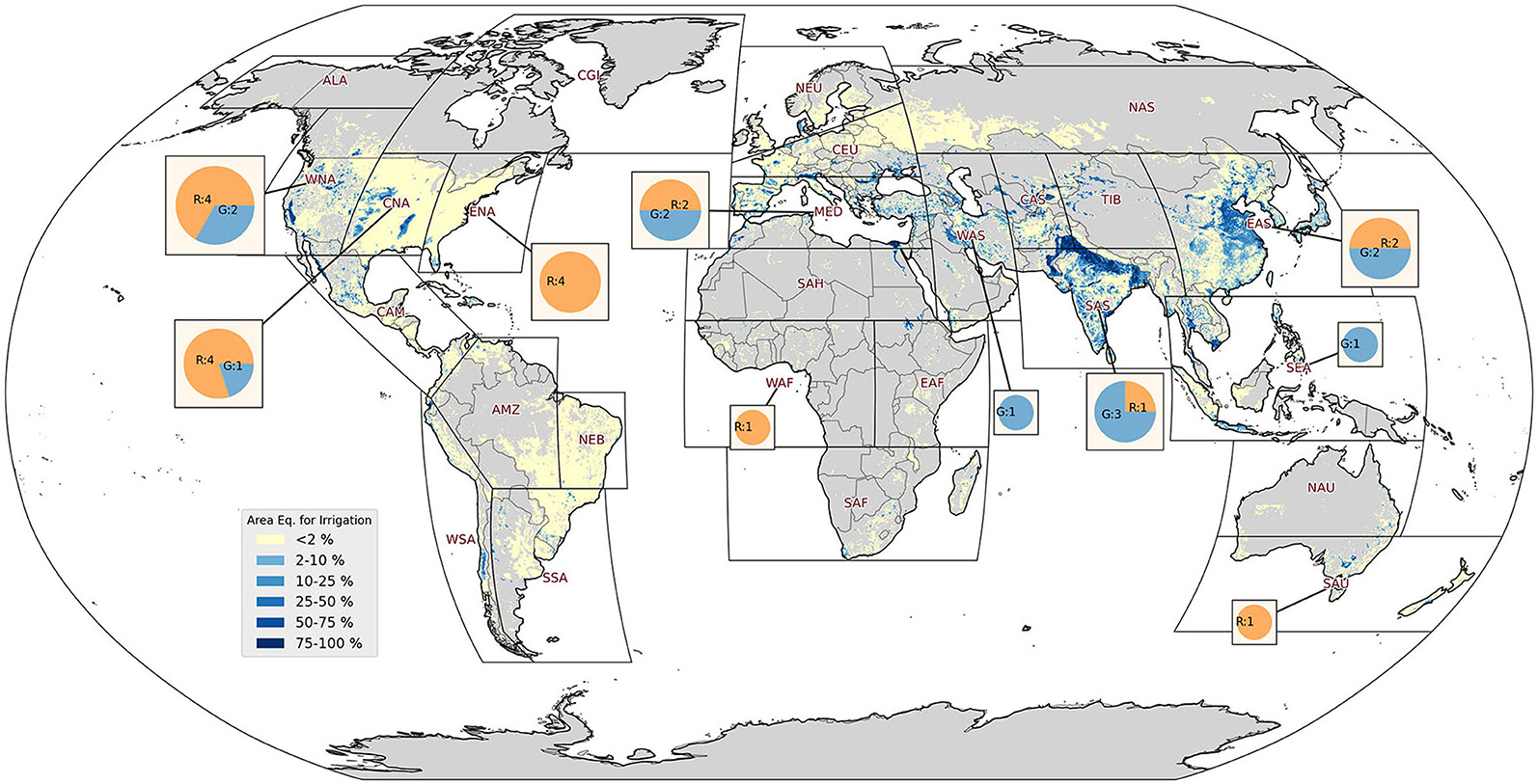
Figure 2. Map of the area equipped for irrigation by Siebert et al. (2013). Pie charts representing the number of studies that report irrigation water amounts for each SREX area, divided in global (blue) and regional (orange).
It should be noted that no study addressed the potential impacts of irrigation in Central- or South-America, despite having areas densely equipped for irrigation (e.g., coastal areas of Northern Mexico, Central Chile). This is all the more surprising as their climate conditions and/or relevance for food security marks them as regions of interest in the context of changing climate and equality.
6.2. New observational datasets
An important limitation on the implementation of irrigation parameterizations and their validation is the lack of appropriate dataset. This involves several aspects such as the extent of the irrigated area in a specific period, spatial information of the main irrigation delivery methods, or the yearly/seasonal water amount used for irrigation as well as the time of application.
In the past, maps of area equipped for irrigation have been generated (Siebert et al., 2005, 2013), which highlight the area that can be potentially be irrigated. These maps are created based on census, so they do not have an annual update, and there is no spatial information on the irrigation delivery methods used. While there are no observational/census dataset that provide the irrigation water amount at least on an annual bases, model-based data are available. To date there are several global dataset that use complex hydrological models to compute the irrigation water requirements, e.g., Döll and Siebert (2002), Siebert and Döll (2010), Wisser et al. (2010), and Wada et al. (2014). These datasets provide irrigation water amount as output at horizontal resolutions of about 55–110 km, with the exception of Siebert and Döll (2010) at about 9 km; for more information refer to Wada et al. (2014). It should, however, be noted that the offline water computation through models has limitations (cf Section 5.1), and only Döll and Siebert (2002) purely rely on observational data as forcing (CRU TS 1.0), while the others use a combination of the CRU dataset and reanalyzes products.
Enhanced dataset together with uncertainty estimates can help to better integrate irrigation as a human activity in Earth system approaches an reanalyzes especially with respect to an enhanced representation of the terrestrial water cycle. Two field campaigns in the recent years have addressed the impact of irrigation on the climate system employing intensive observational periods (IOPs), namely GRAINEX10 (Phillips et al., 2022) and LIAISE11. LIASE field campaign data and review has not been published yet, as it was undergoing in 2021. Irrigation water volumes used during GRAINEX were not available due to policy issues in Nebraska (Christopher Phillips, personal communication). However, the GrainEX IOPs provide a fair good knowledge of the timing and the field locations through indirect observations (Phillips et al., 2022), e.g., soil moisture peaks in absence of precipitation. This concept has also been previously used by Brocca et al. (2014) for the SM2RAIN algorithm, which combines soil moisture satellite products with rainfall estimations to quantify the missing precipitation. The algorithm has been later implemented in Brocca et al. (2018) to better include the irrigation volumes and validate them for pilot sites in the US, Europe and Australia. While this method performed well in periods of low rainfall and if satellites retrieval have low uncertainties, it cannot be applied to sites affected by snow or frozen soil or when rainfall happens throughout the year.
6.3. Applications
The lack of explicit irrigation representation cannot be fully corrected at high resolution in atmospheric reanalyzes products due to the lack of direct soil moisture observations that can be assimilated into the system state and help to correct the vertical water redistribution in the soil. This aspect has already been discussed by Tuinenburg and de Vries (2017) showing significant biases in the ERA-Interim reanalysis. Therefore, irrigation processes needs to be included also in reanalyzes to allow for a correct representation of the Earth system water budget.
When we consider the impact of irrigation on the atmospheric state and dynamics, the effects of the changes range from diurnal to seasonal scales. This is going to impact the weather as well as the seasonal/sub-seasonal predictability with different magnitudes. Most of the predictability improvement is expected to be related to a more suitable soil water content with its importance being summarized in Seneviratne et al. (2010). The impact of irrigation then is further complicated in investigating the multi-year variability, as the volume used is not constant. However, currently only Cook et al. (2015) investigate irrigation as a temporal varying forcing at the spatial resolution of 2o × 2.5o latitude/longitude. While they need this coarse resolution to run a 150-years (1850–200) simulation with 5 ensemble members, it is not enough to capture most of the highly irrigated areas in Europe or the Americas, but only the largest ones in South and East Asia (SAS, EAS).
Even when irrigation itself is included in the studies, there is a lack of quantification of the feedback between different anthropogenic land transitions, such as conversion between cropping systems (McDermid et al., 2017), or the different impacts irrigation can have on Earth system depending on different types of crops. In fact, while effect land management and irrigation has been suggested by several authors as a possible path for climate mitigation (Hirsch et al., 2017), but more work needs to be done in that regard as global models likely underestimates/overestimates the impacts of these practices (Kala and Hirsch, 2020; Jha et al., 2022). In particular, Kala and Hirsch (2020) shows how high albedo crops have higher potentials in Australia than what expected by Hirsch et al. (2017). Similarly, in assuming irrigation has a strong potential for climate mitigation, we neglect both the already existing impact of irrigated lands on climate change (Cook et al., 2011) and the fact that global models likely overestimates its cooling impact (Jha et al., 2022). When these concepts are included in the climate projections and simulations, then the expected increase in water scarcity for the agricultural areas has to be included in limiting the irrigation volumes that can be applied.
Finally, it is crucial to realize that all the down-stream applications that use model or reanalyzes data will benefit from explicitly including irrigation. Specific applications might rely on soil water or near-surface data, where irrigation has the largest effects. Furthermore, all down-stream model and impact assessments that use ESM outputs and refer to agricultural-related processes will strongly benefit [e.g., agricultural drought warnings (Seneviratne et al., 2010), yield calculations (Lobell et al., 2011; Chatzopoulos et al., 2019; Zampieri et al., 2019)].
7. Summary and conclusions
In this review, we presented the developments in the implementations of the irrigation parameterizations for Earth System Models (ESMs).
Irrigation influences various Earth system components and processes partly resulting in feedback effects. While some of these impacts are well-studied, others are not yet fully understood and there is often disagreement on the extent of the impacts in literature. For instance, the IPCC's 5th Assessment Report (AR5) assesses a high confidence on the irrigation cooling effect (e.g., Jia et al., 2019), but its magnitude is not certain. Further, the changes in the surface energy balance are found to affect both the air masses properties and the circulation, potentially causing local and/or remote precipitation feedback. Thus, local anthropogenic changes in the water cycle affect the Earth system at multiple scales. However, while the surface physical feedback of irrigation seems clear, significant uncertainties remains in the quantitative aspects. On the one hand, this uncertainty is related to the underlying soil-atmosphere coupling and its implementation in Earth system models (Seneviratne et al., 2010). On the other hand, the uncertainty can also be ascribed to the irrigation parameterizations themselves and the ambiguity on actual irrigation water amounts among existing research studies.
The currently available parameterizations are collected and classified in Section 3, depending on the activation method (see Section 3.1) and the model quantity that is directly affected (see Section 3.3) by irrigation. While the latter category is more straight-forward from a numerical modeling physical perspective, the activation is crucial due to the anthropogenic nature of the process. Spatially, the irrigation activation is driven mainly by invariant fields, such as the area equipped for irrigation or the crop types. With respect to temporal activation, different concepts are employed, e.g., fixed diurnal irrigation cycle and/or physical thresholds, i.e., soil moisture is falling below a specific threshold. The irrigation water amount is either calculated from available census surveys, modeled dataset or derived from the physical thresholds, as described in Section 3.2.
In the existing studies, four different approaches on how to apply the irrigation water to the model are utilized: (i) to the soil moisture at different depths, (ii) to the surface as precipitation before or after the canopy interception, (iii) to the atmospheric rain water, or (iv) as a water vapor source. A few studies also use a data assimilation approach to implicitly include the effects of irrigation.
Further consideration has been given on how parameterizations relate to the various irrigation delivery methods used in agriculture (summarized in Section 2.1), and to the multiple spatio-temporal scales in the Earth system. While most studies follow an approach to use surface delivery methods or sprinklers that put irrigation water directly onto or below the canopy, one parameterization (see Section 3.3.3) is suitable to also represent the interaction of the sprinkler water with atmospheric processes. However, the employed delivery method has to be adapted to the model's spatio-temporal scale representation (see Section 4.2) and to physical considerations (see Section 4.3). Therefore, the multitude of irrigation parameterizations in literature and their seemingly arbitrary use depending on the scales, is one of the principal causes of the different irrigation water amount estimates (see Section 5.1) and the corresponding uncertainty.
In this review, we have identify some key challenges and opportunities for future developments of irrigation parameterizations. These reach from a consistent inter-model processes representation to a consequent reporting of irrigation amounts (including standardized units, e.g., mms−1), to a realistic water extraction implementation that allows for a closed water budget. The proposed approaches would enable a better process-related estimation of uncertainties across studies, which is currently not possible. Further, they would also allow for broader investigations of the impacts at a climatological scale in the context of a changing climate. The establishment of enhanced observational dataset would also be desirable either for use in independent evaluation efforts or as a more realistic input for the models.
In conclusion, the inclusion of irrigation in Earth system models and the investigation of their effects and feedback processes is an innovative research field that calls for a trans-disciplinary approach involving atmospheric- and soil-physics as well as agro-meteorology and agronomy. A consistent across-scales irrigation framework for Earth system models would strongly benefit weather and seasonal-to-subseasonal forecasts, as well as new reanalyzes and climate prediction. In this regard, the importance of irrigation in the Earth system is further highlighted by the changing climate and its impact on food security, as sustained by the United Nation Sustainable Development Goals (United Nations, 2014). Thus, further advances in irrigation parameterizations may help to address past climate uncertainties, as well as to enhance climate projections, thus, providing better estimates of water scarcity and requirements for food-production in the light of climate change and related adaptation and mitigation strategies.
Author contributions
AV: conceptualization, methodology, and writing—original draft. AV and JK: writing—review and editing. Both authors contributed to the article and approved the submitted version.
Funding
This work has been conducted based on funding by the German Federal Ministry for Digital and Transport (Grant No. BMVI/DWD 4818DWDP5A) and by the Deutsche Forschungsgemeinschaft (DFG, German Research Foundation)—SFB 1502/1-2022—Project No. 450058266.
Conflict of interest
The authors declare that the research was conducted in the absence of any commercial or financial relationships that could be construed as a potential conflict of interest.
Publisher's note
All claims expressed in this article are solely those of the authors and do not necessarily represent those of their affiliated organizations, or those of the publisher, the editors and the reviewers. Any product that may be evaluated in this article, or claim that may be made by its manufacturer, is not guaranteed or endorsed by the publisher.
Footnotes
1. ^Field capacity is defined as the lower limit above which water cannot be held against gravitational drainage. The value depends on the soil type. For further reference, see Seneviratne et al. (2010).
2. ^They refer to 10% above the “stress point,” citing Equation 3 as threshold calculation. However, from the formulation it could not be deduced whether 10% above the 0.5 original threshold, or 10% above the wilting point is intended as stress point.
3. ^The threshold is there incorrectly called “relative soil moisture,” which usually refers to the percentage ratio of the volumetric soil water content against the field capacity (e.g., Su et al., 2003).
4. ^The study does not indicate how the two thresholds are applied differently in the two crop regions of the domain.
5. ^To harmonize the equations in this paper, the derivation of this irrigation scheme is re-written to use the volumetric water content (θ) instead of the absolute water content (W or S), following Seneviratne et al. (2010).
6. ^Defined in the AMS Glossary as: the portion of precipitation that remains in the soil https://glossary.ametsoc.org/wiki/Effective_precipitation.
7. ^This includes also the total amount of water applied as irrigation on the canopy itself.
8. ^https://simplex.giss.nasa.gov/snapshots/
9. ^https://www.lf.uni-bonn.de/en/research/crc-detect
References
Adegoke, J. O., Pielke, R. A., Eastman, J., Mahmood, R., and Hubbard, K. G. (2003). Impact of irrigation on midsummer surface fluxes and temperature under dry synoptic conditions: a regional atmospheric model study of the U.S. high plains. Mon. Weather Rev. 131, 556–564. doi: 10.1175/1520-0493(2003)131andlt
Aegerter, C., Wang, J., Ge, C., Irmak, S., Oglesby, R., Wardlow, B., et al. (2017). Mesoscale modeling of the meteorological impacts of irrigation during the 2012 central plains drought. J. Appl. Meteorol. Climatol. 56, 1259–1283. doi: 10.1175/JAMC-D-16-0292.1
Angelakιs, A. N., Zaccaria, D., Krasilnikoff, J., Salgot, M., Bazza, M., Roccaro, P., et al. (2020). Irrigation of world agricultural lands: evolution through the millennia. Water 12, 1285. doi: 10.3390/w12051285
Barnston, A. G., and Schickedanz, P. T. (1984). The effect of irrigation on warm season precipitation in the southern great plains. J. Clim. Appl. Meteorol. 23, 865–888. doi: 10.1175/1520-0450(1984)023andlt;0865:TEOIOWandgt;2.0.CO;2
Bin Abdullah, K. (2006). Use of water and land for food security and environmental sustainability. Irrigat. Drainage 55, 219–222. doi: 10.1002/ird.254
Bjorneberg, D. (2013). “IRRIGATION | Methods,” in Reference Module in Earth Systems and Environmental Sciences (Elsevier).
Bonfils, C., and Lobell, D. (2007). Empirical evidence for a recent slowdown in irrigation-induced cooling. Proc. Natl. Acad. Sci. U.S.A. 104, 13582–13587. doi: 10.1073/pnas.0700144104
Boucher, O., Myhre, G., and Myhre, A. (2004). Direct human influence of irrigation on atmospheric water vapour and climate. Clim. Dyn. 22, 597–603. doi: 10.1007/s00382-004-0402-4
Bradley, K., Scharf, P. C., and Luce, G. A. (2017). “Integrated pest and crop management,” in MU Integrated Pest Management Program of the Division of Plant Sciences Extension, Vol. 27. doi: 10.1111/gcb.14628
Brocca, L., Ciabatta, L., Massari, C., Moramarco, T., Hahn, S., Hasenauer, S., et al. (2014). Soil as a natural rain gauge: estimating global rainfall from satellite soil moisture data. J. Geophys. Res. Atmospher.119, 5128–5141. doi: 10.1002/2014JD021489
Brocca, L., Tarpanelli, A., Filippucci, P., Dorigo, W., Zaussinger, F., Gruber, A., et al. (2018). How much water is used for irrigation? A new approach exploiting coarse resolution satellite soil moisture products. Int. J. Appl. Earth Observat. Geoinf. 73, 752–766. doi: 10.1016/j.jag.2018.08.023
Brouwer, C., Prins, K., Kay, M., and Heibloem, M. (1985b). Irrigation Water Management: Training Manual No. 5: Irrigation methods.
Brouwer, C., Prins, K., Kay, M., and Heibloem, M. (1985a). Irrigation Water Management: Training Manual No. 1: Introduction to Irrigation. Available online at: https://www.fao.org/3/r4082e/r4082e00.htm
Brown, J. F., and Pervez, M. S. (2014). Merging remote sensing data and national agricultural statistics to model change in irrigated agriculture. Agric. Syst. 127, 28–40. doi: 10.1016/j.agsy.2014.01.004
Budyko, M. I. (1972). The future climate. Eos Trans. Am. Geophys. Union 53, 868. doi: 10.1029/EO053i010p00868
Chase, T. N. Sr, R. A. P., Kittel, T. G. F., Baron, J. S., and Stohlgren, T. J. (1999). Potential impacts on Colorado Rocky Mountain weather due to land use changes on the adjacent Great Plains. J. Geophys. Res. 104, 16673–16690. doi: 10.1029/1999JD900118
Chatzopoulos, T., Pérez Domínguez, I., Zampieri, M., and Toreti, A. (2019). Climate extremes and agricultural commodity markets: a global economic analysis of regionally simulated events. Weather Clim. Extremes 27, 100193. doi: 10.1016/j.wace.2019.100193
Cheng, Y., Huang, M., Zhu, B., Bisht, G., Zhou, T., Liu, Y., et al. (2021). Validation of the community land model version 5 over the contiguous United States (CONUS) using in situ and remote sensing data sets. J. Geophys. Res. Atmospher. 126, e2020JD033539. doi: 10.1029/2020JD033539
Cook, B. I., McDermid, S. S., Puma, M. J., Williams, A. P., Seager, R., Kelley, M., et al. (2020). Divergent regional climate consequences of maintaining current irrigation rates in the 21st century. J. Geophys. Res. Atmospher. 125, e2019JD031814. doi: 10.1029/2019JD031814
Cook, B. I., Puma, M. J., and Krakauer, N. Y. (2011). Irrigation induced surface cooling in the context of modern and increased greenhouse gas forcing. Clim. Dyn. 37, 1587–1600. doi: 10.1007/s00382-010-0932-x
Cook, B. I., Shukla, S. P., Puma, M. J., and Nazarenko, L. S. (2015). Irrigation as an historical climate forcing. Clim. Dyn. 44, 1715–1730. doi: 10.1007/s00382-014-2204-7
Dari, J., Quintana-Seguí, P., Escorihuela, M. J., Stefan, V., Brocca, L., and Morbidelli, R. (2021). Detecting and mapping irrigated areas in a Mediterranean environment by using remote sensing soil moisture and a land surface model. J. Hydrol. 596, 126129. doi: 10.1016/j.jhydrol.2021.126129
De Ridder, K., and Gallée, H. (1998). Land surface-induced regional climate change in southern Israel. J. Appl. Meteorol. 37, 1470–1485. doi: 10.1175/1520-0450(1998)037andlt;1470:LSIRCCandgt;2.0.CO;2
de Rosnay, P. (2003). Integrated parameterization of irrigation in the land surface model ORCHIDEE. Validation over Indian Peninsula. Geophys. Res. Lett. 30, 1986. doi: 10.1029/2003GL018024
de Vrese, P., and Hagemann, S. (2018). Uncertainties in modelling the climate impact of irrigation. Clim. Dyn. 51, 2023–2038. doi: 10.1007/s00382-017-3996-z
de Vrese, P., Stacke, T., and Hagemann, S. (2018). Exploring the biogeophysical limits of global food production under different climate change scenarios. Earth Syst. Dyn. 9, 393–412. doi: 10.5194/esd-9-393-2018
de Vries, D. A. (1959). The influence of irrigation on the energy balance and the climate near the ground. J. Meteorol. 16, 256–270. doi: 10.1175/1520-0469(1959)016andlt;0256:TIOIOTandgt;2.0.CO;2
Deangelis, A., Dominguez, F., Fan, Y., Robock, A., Kustu, M. D., and Robinson, D. (2010). Evidence of enhanced precipitation due to irrigation over the Great Plains of the United States. J. Geophys. Res. Atmospher. 115, D15115. doi: 10.1029/2010JD013892
Decker, M., Ma, S., and Pitman, A. (2017). Local land-atmosphere feedbacks limit irrigation demand. Environ. Res. Lett. 12, 054003. doi: 10.1088/1748-9326/aa65a6
Döll, P., Hoffmann-Dobrev, H., Portmann, F. T., Siebert, S., Eicker, A., Rodell, M., et al. (2012). Impact of water withdrawals from groundwater and surface water on continental water storage variations. J. Geodyn. 59–60, 143–156. doi: 10.1016/j.jog.2011.05.001
Döll, P., and Siebert, S. (2002). Global modeling of irrigation water requirements. Water Resour. Res. 38, 8–1. doi: 10.1029/2001WR000355
Douglas, E. M., Beltrán-Przekurat, A., Niyogi, D., Pielke, R. A., and Vörösmarty, C. J. (2009). The impact of agricultural intensification and irrigation on land-atmosphere interactions and Indian monsoon precipitation-A mesoscale modeling perspective. Glob. Planet Change 67, 117–128. doi: 10.1016/j.gloplacha.2008.12.007
Evans, J. P., and Zaitchik, B. F. (2008). Modeling the large-scale water balance impact of different irrigation systems. Water Resour. Res. 44, 6671. doi: 10.1029/2007WR006671
Flohn, H. (1963). “Theories of climatic chance from the viewpoint of the global energy budget,” in Changes of Climate, Proceedings of the Rome Symposium for UNESCO and World Meterological Organization, ed UNESCO, 339–344. Available online at: https://unesdoc.unesco.org/ark:/48223/pf0000069895
Gates, W. L., Boyle, J. S., Covey, C., Dease, C. G., Doutriaux, C. M., Drach, R. S., et al. (1999). An overview of the results of the atmospheric model intercomparison project (AMIP I). Bull. Am. Meteorol. Soc. 80, 29–55. doi: 10.1175/1520-0477(1999)080andlt;0029:AOOTROandgt;2.0.CO;2
Girotto, M., De Lannoy, G. J. M., Reichle, R. H., Rodell, M., Draper, C., Bhanja, S. N., et al. (2017). Benefits and pitfalls of GRACE data assimilation: a case study of terrestrial water storage depletion in India. Geophys. Res. Lett. 44, 4107–4115. doi: 10.1002/2017GL072994
Gramlich, A., Stoll, S., Stamm, C., Walter, T., and Prasuhn, V. (2018). Effects of artificial land drainage on hydrology, nutrient and pesticide fluxes from agricultural fields-A review. Agric. Ecosyst. Environ. 266, 84–99. doi: 10.1016/j.agee.2018.04.005
Guimberteau, M., Laval, K., Perrier, A., and Polcher, J. (2012). Global effect of irrigation and its impact on the onset of the Indian summer monsoon. Clim. Dyn. 39, 1329–1348. doi: 10.1007/s00382-011-1252-5
Haddeland, I., Lettenmaier, D. P., and Skaugen, T. (2006). Effects of irrigation on the water and energy balances of the Colorado and Mekong river basins. J. Hydrol. 324, 210–223. doi: 10.1016/j.jhydrol.2005.09.028
Harding, K. J., Twine, T. E., and Lu, Y. (2015). Effects of dynamic crop growth on the simulated precipitation response to irrigation*. Earth Interact. 19, 1–31. doi: 10.1175/EI-D-15-0030.1
Hirsch, A. L., Wilhelm, M., Davin, E. L., Thiery, W., and Seneviratne, S. I. (2017). Can climate-effective land management reduce regional warming? J. Geophys. Res. Atmospher. 122, 2269–2288. doi: 10.1002/2016JD026125
Im, E.-S., and Eltahir, E. A. B. (2014). Enhancement of rainfall and runoff upstream from irrigation location in a climate model of West Africa. Water Resour. Res. 50, 8651–8674. doi: 10.1002/2014W.R.015592
Irmak, S. (2018). Subirrigation in Agricultural Fields. Technical report, Nebraska Extension Publications.
Jha, R., Mondal, A., Devanand, A., Roxy, M. K., and Ghosh, S. (2022). Limited influence of irrigation on pre-monsoon heat stress in the Indo-Gangetic Plain. Nat. Commun. 13, 1–10. doi: 10.1038/s41467-022-31962-5
Jia, G., Shevliakova, E., Artaxo, P., De Noblet-Ducoudré, N., Houghton, R., House, J., et al. (2019). “Land-climate interactions,” in Climate Change and Land: An IPCC Special Report on Climate Change, Desertification, Land Degradation, Sustainable Land Management, Food Security, and Greenhouse Gas Fluxes in Terrestrial Ecosystems, eds P. R. Shukla, J. Skea, E. Calvo Buendia, V. Masson-Delmotte, H.-O. Pörtner, D. C. Roberts, P. Zhai, R. Slade, S. Connors, R. van Diemen, M. Ferrat, E. Haughey, S. Luz, S. Neogi, M. Pathak, J. Petzold, J. Portugal Pereira, P. Vyas, E. Huntley, K. Kissick, M, Belkacemi, J. Malley.
Kala, J., and Hirsch, A. L. (2020). Could crop albedo modification reduce regional warming over Australia? Weather Clim. Extremes 30, 100282. doi: 10.1016/j.wace.2020.100282
Kanamaru, H., and Kanamitsu, M. (2008). Model diagnosis of nighttime minimum temperature warming during summer due to irrigation in the california central valley. J. Hydrometeorol. 9, 1061–1072. doi: 10.1175/2008JHM967.1
Kang, S., and Eltahir, E. A. B. (2018). North China plain threatened by deadly heatwaves due to climate change and irrigation. Nat. Commun. 9, 2894. doi: 10.1038/s41467-018-05252-y
Kimaro, J. G., Scharsich, V., Kolb, A., Huwe, B., and Bogner, C. (2019). Distribution of traditional irrigation canals and their discharge dynamics at the southern slopes of Mount Kilimanjaro. Front. Environ. Sci. 7, 24. doi: 10.3389/fenvs.2019.00024
Kirkham, M. (2005). “Field capacity, wilting point, available water, and the non-limiting water range,” in Principles of Soil and Plant Water Relations (Elsevier), 101–115. Available online at: https://www.sciencedirect.com/science/article/pii/B9780124097513500086?via%3Dihub
Krakauer, N. Y., Puma, M. J., Cook, B. I., Gentine, P., and Nazarenko, L. (2016). Ocean-atmosphere interactions modulate irrigation's climate impacts. Earth Syst. Dyn. 7, 863–876. doi: 10.5194/esd-7-863-2016
Kueppers, L. M., Snyder, M. A., and Sloan, L. C. (2007). Irrigation cooling effect: regional climate forcing by land-use change. Geophys. Res. Lett. 34, L03703. doi: 10.1029/2006GL028679
Kueppers, L. M., Snyder, M. A., Sloan, L. C., Cayan, D., Jin, J., Kanamaru, H., et al. (2008). Seasonal temperature responses to land-use change in the western United States. Glob. Planet Change 60, 250–264. doi: 10.1016/j.gloplacha.2007.03.005
Lawston, P. M., Santanello, J. A., and Kumar, S. V. (2017). Irrigation signals detected from SMAP soil moisture retrievals. Geophys. Res. Lett. 44, 860–811. doi: 10.1002/2017GL075733
Lawston, P. M., Santanello, J. A., Zaitchik, B. F., and Rodell, M. (2015). Impact of irrigation methods on land surface model spinup and initialization of WRF forecasts. J. Hydrometeorol. 16, 1135–1154. doi: 10.1175/JHM-D-14-0203.1
Lee, E., Sacks, W. J., Chase, T. N., and Foley, J. A. (2011). Simulated impacts of irrigation on the atmospheric circulation over Asia. J. Geophys. Res. 116, D08114. doi: 10.1029/2010JD014740
Lee, P., and Ngan, F. (2011). Coupling of important physical processes in the planetary boundary layer between meteorological and chemistry models for regional to continental scale air quality forecasting: an overview. Atmospher. 2, 464–483. doi: 10.3390/atmos2030464
Leng, G., Huang, M., Tang, Q., Gao, H., and Leung, L. R. (2014). Modeling the effects of groundwater-fed irrigation on terrestrial hydrology over the conterminous United States. J. Hydrometeorol. 15, 957–972. doi: 10.1175/JHM-D-13-049.1
Leng, G., Huang, M., Tang, Q., Sacks, W. J., Lei, H., and Leung, L. R. (2013). Modeling the effects of irrigation on land surface fluxes and states over the conterminous United States: sensitivity to input data and model parameters. J. Geophys. Res. tmospheres 118, 9789–9803. doi: 10.1002/jgrd.50792
Leng, G., Leung, L. R., and Huang, M. (2017). Significant impacts of irrigation water sources and methods on modeling irrigation effects in the ACME land model. J. Adv. Model. Earth Syst. 9, 1665–1683. doi: 10.1002/2016MS000885
Leng, G., Tang, Q., Huang, M., and Leung, L.-Y. R. (2015). A comparative analysis of the impacts of climate change and irrigation on land surface and subsurface hydrology in the North China Plain. Regional Environ. Change 15, 251–263. doi: 10.1007/s10113-014-0640-x
Liu, G., Wang, W., Shao, Q., Wei, J., Zheng, J., Liu, B., et al. (2021). Simulating the climatic effects of irrigation over china by using the WRF-noah model system with mosaic approach. J. Geophys. Res. Atmospher. 126, e2020JD034428. doi: 10.1029/2020JD034428
Liu, X., Liu, W., Tang, Q., Liu, B., Wada, Y., and Yang, H. (2022). Global agricultural water scarcity assessment incorporating blue and green water availability under future climate change. Earths Future 10, e2021EF002567. doi: 10.1029/2021EF002567
Lo, M., and Famiglietti, J. S. (2013). Irrigation in California's central valley strengthens the southwestern U.S. water cycle. Geophys. Res. Lett. 40, 301–306. doi: 10.1002/grl.50108
Lobell, D., Bala, G., Mirin, A., Phillips, T., Maxwell, R., and Rotman, D. (2009). Regional differences in the influence of irrigation on climate. J. Clim. 22, 2248–2255. doi: 10.1175/2008JCLI2703.1
Lobell, D. B., Bala, G., Bonfils, C., and Duffy, P. B. (2006a). Potential bias of model projected greenhouse warming in irrigated regions. Geophys. Res. Lett. 33, L13709. doi: 10.1029/2006GL026770
Lobell, D. B., Bala, G., and Duffy, P. B. (2006b). Biogeophysical impacts of cropland management changes on climate. Geophys. Res. Lett. 33, L06708. doi: 10.1029/2005GL025492
Lobell, D. B., Bonfils, C., and Faurès, J. -M. (2008). The role of irrigation expansion in past and future temperature trends. Earth Interact. 12, 1–11. doi: 10.1175/2007EI241.1
Lobell, D. B., Schlenker, W., and Costa-Roberts, J. (2011). Climate trends and global crop production since 1980. Science 333, 616–620. doi: 10.1126/science.1204531
Lohar, D., and Pal, B. (1995). The effect of irrigation on premonsoon season precipitation over South West Bengal, India. J. Clim. 8, 2567–2570. doi: 10.1175/1520-0442(1995)008andlt;2567:TEOIOPandgt;2.0.CO;2
Lu, Y., Harding, K., and Kueppers, L. (2017). Irrigation effects on land-atmosphere coupling strength in the United States. J. Clim. 30, 3671–3685. doi: 10.1175/JCLI-D-15-0706.1
Lu, Y., Jin, J., and Kueppers, L. M. (2015). Crop growth and irrigation interact to influence surface fluxes in a regional climate-cropland model (WRF3.3-CLM4crop). Clim. Dyn. 45, 3347–3363. doi: 10.1007/s00382-015-2543-z
Luyssaert, S., Jammet, M., Stoy, P. C., Estel, S., Pongratz, J., Ceschia, E., et al. (2014). Land management and land-cover change have impacts of similar magnitude on surface temperature. Nat. Clim. Chang 4, 389–393. doi: 10.1038/nclimate2196
Mahmood, R., Hubbard, K. G., Leeper, R. D., and Foster, S. A. (2008). Increase in near-surface atmospheric moisture content due to land use changes: evidence from the observed dewpoint temperature data. Mon. Weather Rev. 136, 1554–1561. doi: 10.1175/2007MWR2040.1
Mahmood, R., Pielke, R. A., Hubbard, K. G., Niyogi, D., Dirmeyer, P. A., Mcalpine, C., et al. (2014). Land cover changes and their biogeophysical effects on climate. Int. J. Climatol. 34, 929–953. doi: 10.1002/joc.3736
Manabe, S., Smagorinsky, J., Strickler, R. F., Manabe, S., Smagorinsky, J., and Strickler, R. F. (1965). Simulated climatology of a general circulation model with a hydrologic cycle. Mon. Weather Rev. 93, 769–798. doi: 10.1175/1520-0493(1965)093andlt;0769:SCOAGCandgt;2.3.CO;2
Manik, S. M., Pengilley, G., Dean, G., Field, B., Shabala, S., and Zhou, M. (2019). Soil and crop management practices to minimize the impact of waterlogging on crop productivity. Front. Plant Sci. 10:140. doi: 10.3389/fpls.2019.00140
Marcella, M. P., and Eltahir, E. A. (2014). Introducing an irrigation scheme to a regional climate model: a case study over West Africa. J. Clim. 27, 5708–5723. doi: 10.1175/JCLI-D-13-00116.1
McDermid, S. S., Mearns, L. O., and Ruane, A. C. (2017). Representing agriculture in Earth system models: approaches and priorities for development. J. Adv. Model. Earth Syst. 9, 2230–2265. doi: 10.1002/2016MS000749
Milly, P. C. D., and Dunne, K. A. (1994). Sensitivity of the global water cycle to the water-holding capacity of land. J. Clim. 7, 506–526. doi: 10.1175/1520-0442(1994)007andlt;0506:SOTGWCandgt;2.0.CO;2
Moghazi, H. E., and Ismail, E. S. (1997). A study of losses from field channels under arid region conditions. Irrigat. Sci. 17, 105–110. doi: 10.1007/s002710050028
Nie, W., Zaitchik, B. F., Rodell, M., Kumar, S. V., Arsenault, K. R., and Badr, H. S. (2021). Irrigation water demand sensitivity to climate variability across the contiguous united states. Water Resour. Res. 57, 2020WR027738. doi: 10.1029/2020WR027738
Nie, W., Zaitchik, B. F., Rodell, M., Kumar, S. V., Arsenault, K. R., Li, B., et al. (2019). Assimilating GRACE into a land surface model in the presence of an irrigation-induced groundwater trend. Water Resour. Res. 55, 11274–11294. doi: 10.1029/2019WR025363
Oleson, K., Lawrence, D. M., Bonan, G. B., Drewniak, B., Huang, M., Koven, C. D., et al. (2013). Technical description of version 4.5 of the Community Land Model (CLM) (No. NCAR/TN-503+STR). doi: 10.5065/D6RR1W7M
Ozdogan, M., and Gutman, G. (2008). A new methodology to map irrigated areas using multi-temporal MODIS and ancillary data: an application example in the continental US. Remote Sens. Environ. 112, 3520–3537. doi: 10.1016/j.rse.2008.04.010
Ozdogan, M., Rodell, M., Beaudoing, H. K., and Toll, D. L. (2009). Simulating the effects of irrigation over the United States in a land surface model based on satellite-derived agricultural data. J. Hydrometeorol. 11, 171–184. doi: 10.1175/2009JHM1116.1
Ozdogan, M., Salvucci, G. D., and Anderson, B. T. (2006). Examination of the Bouchet-Morton complementary relationship using a mesoscale climate model and observations under a progressive irrigation scenario. J. Hydrometeorol. 7, 235–251. doi: 10.1175/JHM485.1
Panda, D., and Barik, J. (2021). Flooding tolerance in rice: focus on mechanisms and approaches. Rice Sci. 28, 43–57. doi: 10.1016/j.rsci.2020.11.006
Pei, L., Moore, N., Zhong, S., Kendall, A. D., Gao, Z., and Hyndman, D. W. (2016). Effects of irrigation on summer precipitation over the United States. J. Clim. 29, 3541–3558. doi: 10.1175/JCLI-D-15-0337.1
Pei, L., Moore, N., Zhong, S., Luo, L., Hyndman, D. W., Heilman, W. E., et al. (2014). WRF model sensitivity to land surface model and cumulus parameterization under short-term climate extremes over the Southern great plains of the United States. J. Clim. 27, 7703–7724. doi: 10.1175/JCLI-D-14-00015.1
Pervez, M. S., and Brown, J. F. (2010). Mapping irrigated lands at 250-m scale by merging MODIS data and National Agricultural Statistics. Remote Sens. 2, 2388–2412. doi: 10.3390/rs2102388
Phillips, C. E., Nair, U. S., Mahmood, R., Rappin, E., and Pielke, R. A. (2022). Influence of irrigation on diurnal mesoscale circulations: results from GRAINEX. Geophys. Res. Lett. 49, e2021GL096822. doi: 10.1029/2021GL096822
Phocaides, A. (2000). Technical handbook on pressurized irrigation techniques. Technical report, Food and Agriculture Organizationof the United Nations.
Pielke, R. A., Adegoke, J. O., Chase, T. N., Marshall, C. H., Matsui, T., and Niyogi, D. (2007). A new paradigm for assessing the role of agriculture in the climate system and in climate change. Agric. Forest Meteorol. 142, 234–254. doi: 10.1016/j.agrformet.2006.06.012
Pielke, R. A., and Zeng, X. (1989). Influence on severe storm development of irrigated land. Natl. Weather Digest 14, 16–17.
Portmann, F. T., Siebert, S., and Döll, P. (2010). MIRCA2000-Global monthly irrigated and rainfed crop areas around the year 2000: a new high-resolution data set for agricultural and hydrological modeling. Glob. Biogeochem. Cycles 24, 3435. doi: 10.1029/2008GB003435
Prein, A. F., Rasmussen, R. M., Wang, D., and Giangrande, S. E. (2021). Sensitivity of organized convective storms to model grid spacing in current and future climates. Philos. Trans. A Math. Phys. Eng. Sci. 379, 20190546. doi: 10.1098/rsta.2019.0546
Puma, M. J., and Cook, B. I. (2010). Effects of irrigation on global climate during the 20th century. J. Geophys. Res. 115, D16120. doi: 10.1029/2010JD014122
Qian, Y., Huang, M., Yang, B., and Berg, L. K. (2013). A modeling study of irrigation effects on surface fluxes and land-air-cloud interactions in the southern great plains. J. Hydrometeorol. 14, 700–721. doi: 10.1175/JHM-D-12-0134.1
Sacks, W. J., Cook, B. I., Buenning, N., Levis, S., and Helkowski, J. H. (2009). Effects of global irrigation on the near-surface climate. Clim. Dyn. 33, 159–175. doi: 10.1007/s00382-008-0445-z
Saeed, F., Hagemann, S., and Jacob, D. (2009). Impact of irrigation on the South Asian summer monsoon. Geophys. Res. Lett. 36, L20711. doi: 10.1029/2009GL040625
Salmon, J., Friedl, M. A., Frolking, S., Wisser, D., and Douglas, E. M. (2015). Global rain-fed, irrigated, and paddy croplands: a new high resolution map derived from remote sensing, crop inventories and climate data. Int. J. Appl. Earth Observat. Geoinf. 38, 321–334. doi: 10.1016/j.jag.2015.01.014
Schättler, U., Doms, G., and Schraff, C. (2018). A Description of the Nonhydrostatic Regional COSMO-Model Part VII : User's Guide. Technical report.
Segal, M., Pan, Z., Turner, R. W., and Takle, E. S. (1998). On the potential impact of irrigated areas in North America on summer rainfall caused by large-scale systems. J. Appl. Meteorol. Climatol. 37, 325–331. doi: 10.1175/1520-0450-37.3.325
Seneviratne, S. I., Corti, T., Davin, E. L., Hirschi, M., Jaeger, E. B., Lehner, I., et al. (2010). Investigating soil moisture-climate interactions in a changing climate: a review. Earth Sci. Rev. 99, 125–161. doi: 10.1016/j.earscirev.2010.02.004
Seth, A., Rauscher, S. A., Camargo, S. J., Qian, J. H., and Pal, J. S. (2007). RegCM3 regional climatologies for South America using reanalysis and ECHAM global model driving fields. Clim. Dyn. 28, 461–480. doi: 10.1007/s00382-006-0191-z
Siebert, S., and Döll, P. (2010). Quantifying blue and green virtual water contents in global crop production as well as potential production losses without irrigation. J. Hydrol. 384, 198–217. doi: 10.1016/j.jhydrol.2009.07.031
Siebert, S., DöllP Hoogeveen, J., Faures, J. M., Frenken, K., and Feick, S. (2005). Development and validation of the global map of irrigation areas. Hydrolo. Earth Syst. Sci. 9, 535–547. doi: 10.5194/hess-9-535-2005
Siebert, S., Henrich, V., Frenken, K., and Burke, J. (2013). Global Map of Irrigation Areas Version 5. Food and Agriculture Organization of the United Nations.
Singh, D., McDermid, S. P., Cook, B. I., Puma, M. J., Nazarenko, L., and Kelley, M. (2018). Distinct influences of land cover and land management on seasonal climate. J. Geophys. Res. Atmospher. 123, 017–012. doi: 10.1029/2018JD028874
Skamarock, W., Klemp, J., Dudhi, J., Gill, D., Barker, D., Duda, M., et al. (2008). A Description of the Advanced Research WRF Version 3. Technical Report, 113.
Smirnova, T. G., Brown, J. M., Benjamin, S. G., and Kenyon, J. S. (2016). Modifications to the Rapid Update Cycle land surface model (RUC LSM) available in the weather research and forecasting (WRF) model. Mon. Weather Rev. 144, 1851–1865. doi: 10.1175/MWR-D-15-0198.1
Sorooshian, S., Li, J., Hsu, K.-L., and Gao, X. (2011). How significant is the impact of irrigation on the local hydroclimate in Californias Central Valley? Comparison of model results with ground and remote-sensing data. J. Geophys. Res. 116, D06102. doi: 10.1029/2010JD014775
Sorooshian, S., Li, J., Hsu, K.-L., and Gao, X. (2012). Influence of irrigation schemes used in regional climate models on evapotranspiration estimation: results and comparative studies from California's Central Valley agricultural regions. J. Geophys. Res. Atmospher. 117, 16978. doi: 10.1029/2011JD016978
Squatriti, P. (1998). “The wet and the dry: water in agriculture,” in Water and Society in Early Medieval Italy, AD 400–1000 (Cambridge: Cambridge University Press), 66–96.
Sridhar, V. (2013). Tracking the influence of irrigation on land surface fluxes and boundary layer climatology. J. Contemporary Water Res. Educ. 152, 79–93. doi: 10.1111/j.1936-704X.2013.03170.x
Su, Z., Yacob, A., Wen, J., Roerink, G., He, Y., Gao, B., et al. (2003). Assessing relative soil moisture with remote sensing data: theory, experimental validation, and application to drought monitoring over the North China Plain. Phys. Chem. Earth 28, 89–101. doi: 10.1016/S1474-7065(03)00010-X
Thiery, W., Davin, E. L., Lawrence, D. M., Hirsch, A. L., Hauser, M., and Seneviratne, S. I. (2017). Present-day irrigation mitigates heat extremes. J. Geophys. Res. Atmospher. 122, 1403–1422. doi: 10.1002/2016JD025740
Thiery, W., Visser, A. J., Fischer, E. M., Hauser, M., Hirsch, A. L., Lawrence, D. M., et al. (2020). Warming of hot extremes alleviated by expanding irrigation. Nat. Commun. 11, 1–7. doi: 10.1038/s41467-019-14075-4
Tuinenburg, O. A., and de Vries, J. P. R. (2017). Irrigation patterns resemble ERA-interim reanalysis soil moisture additions. Geophys. Res. Lett. 44, 341–310. doi: 10.1002/2017GL074884
Tuinenburg, O. A., Hutjes, R. W. A., Stacke, T., Wiltshire, A., and Lucas-Picher, P. (2014). Effects of irrigation in india on the atmospheric water budget. J. Hydrometeorol. 15, 1028–1050. doi: 10.1175/JHM-D-13-078.1
United Nations (2014). Transforming our world: The 2030 agenda for sustainable development. Technical report.
Valmassoi, A., Dudhia, J., Di Sabatino, S., and Pilla, F. (2020a). Evaluation of three new surface irrigation parameterizations in the WRF-ARW v3.8.1 model: the Po Valley (Italy) case study. Geosci. Model Dev. 13, 3179–3201. doi: 10.5194/gmd-13-3179-2020
Valmassoi, A., Dudhia, J., Di Sabatino, S., and Pilla, F. (2020b). Irrigation impact on precipitation during a heatwave event using WRF-ARW: the summer 2015 Po Valley case. Atmospher. Res. 241, 104951. doi: 10.1016/j.atmosres.2020.104951
Valmassoi, A., Dudhia, J., Di Sabatino, S., and Pilla, F. (2020c). Regional climate impacts of irrigation in northern Italy using a high resolution model. Atmosphere 11, 72. doi: 10.3390/atmos11010072
van Oldenborgh, G. J., Collins, M., Arblaster, J., Christensen, J. H., Marotzke, J., Power, S. B., et al. (2014). “Annex I: atlas of global and regional climate projections,” in Contribution of Working Group I to the Fifth Assessment Report of the Intergovernmental Panel on Climate Change, Chapter Annex 1, eds T. F. Stocker, D. Qin, G.-K. Plattner, M. Tignor, S. K. Allen, J. Boschung, A. Nauels, Y. Xia, V. Bex, P. M. Midgley (Cambridge: Cambridge University Press).
Wada, Y., Wisser, D., and Bierkens, M. F. P. (2014). Global modeling of withdrawal, allocation and consumptive use of surface water and groundwater resources. Earth Syst. Dyn. 5, 15–40. doi: 10.5194/esd-5-15-2014
Wada, Y., Wisser, D., Eisner, S., Flörke, M., Gerten, D., Haddeland, I., et al. (2013). Multimodel projections and uncertainties of irrigation water demand under climate change. Geophys. Res. Lett. 40, 4626–4632. doi: 10.1002/grl.50686
Wei, J., Dirmeyer, P. A., Wisser, D., Bosilovich, M. G., and Mocko, D. M. (2013). Where does the irrigation water go? An estimate of the contribution of irrigation to precipitation using MERRA. J. Hydrometeorol. 14, 275–289. doi: 10.1175/JHM-D-12-079.1
Wisser, D., Fekete, B. M., Vörösmarty, C. J., and Schumann, A. H. (2010). Reconstructing 20th century global hydrography: a contribution to the Global Terrestrial Network- Hydrology (GTN-H). Hydrol. Earth Syst. Sci. 14, 1–24. doi: 10.5194/hess-14-1-2010
Wisser, D., Frolking, S., Douglas, E. M., Fekete, B. M., Vörösmarty, C. J., and Schumann, A. H. (2008). Global irrigation water demand: variability and uncertainties arising from agricultural and climate data sets. Geophys. Res. Lett. 35, 35296. doi: 10.1029/2008GL035296
Wu, L., Feng, J., and Miao, W. (2018). Simulating the impacts of irrigation and dynamic vegetation over the north china plain on regional climate. J. Geophys. Res. Atmospher. 123, 8017–8034. doi: 10.1029/2017JD027784
Yang, B., Zhang, Y., Qian, Y., Tang, J., and Liu, D. (2016). Climatic effects of irrigation over the Huang-Huai-Hai Plain in China simulated by the weather research and forecasting model. J. Geophys. Res. Atmospher. 121, 2246–2264. doi: 10.1002/2015JD023736
Yang, Z., Dominguez, F., Zeng, X., Hu, H., Gupta, H., and Yang, B. (2017). Impact of irrigation over the california central valley on regional climate. J. Hydrometeorol. 18, 1341–1357. doi: 10.1175/JHM-D-16-0158.1
Zampieri, M., Ceglar, A., Dentener, F., Dosio, A., Naumann, G., Van Den Berg, M., et al. (2019). When will current climate extremes affecting maize production become the norm? Earths Future 7, 113–122. doi: 10.1029/2018EF000995
Keywords: irrigation, irrigation parameterization, earth system modeling, irrigation-effect on weather, atmospheric model
Citation: Valmassoi A and Keller JD (2022) A review on irrigation parameterizations in Earth system models. Front. Water 4:906664. doi: 10.3389/frwa.2022.906664
Received: 28 March 2022; Accepted: 24 October 2022;
Published: 16 November 2022.
Edited by:
Rishikesh Singh, Panjab University, IndiaReviewed by:
Xi Chen, University of Cincinnati, United StatesHyunglok Kim, University of Virginia, United States
Copyright © 2022 Valmassoi and Keller. This is an open-access article distributed under the terms of the Creative Commons Attribution License (CC BY). The use, distribution or reproduction in other forums is permitted, provided the original author(s) and the copyright owner(s) are credited and that the original publication in this journal is cited, in accordance with accepted academic practice. No use, distribution or reproduction is permitted which does not comply with these terms.
*Correspondence: Arianna Valmassoi, avalmass@uni-bonn.de