 Jérémy Guilhen1,2*
 Marie Parrens3,4
 Sabine Sauvage1*William Santini5Franck Mercier2
 Ahmad Al Bitar3Clément Fabre6Jean-Michel Martinez5
 José-Miguel Sànchez-Pérez1
- 1Laboratoire Écologie Fonctionnelle et Environnement, Institut National Polytechnique de Toulouse, Centre National de la Recherche Scientifique (CNRS), Université de Toulouse (UPS), Toulouse, France
- 2Collecte Localisation Satelittes, Toulouse, France
- 3Centre d'Études Spatiales de la Biosphère, Centre National d'Études Spatiales, Universitè de Toulouse (UPS), Toulouse, France
- 4Dynafor, Université de Toulouse, Institut National de Recherche pour l'Agriculture, l'Alimentation et l'Environnement, Institut National Polytechnique de Toulouse, Institut National Polytechnique-PURPAN, Castanet-Tolosan, France
- 5Institut de Recherche pour le Développement, Laboratoire GET (IRD, Centre National de la Recherche Scientifique, Université de Toulouse, Centre National d'Études Spatiales), Toulouse, France
- 6Eawag, Swiss Federal Institute of Aquatic Science and Technology, Dubendorf, Switzerland
The Madeira is one of the major tributaries of the Amazon River and is characterized by a large alluvial floodplain throughout the stream continuum. This study aims to better assess the hydrological functioning of the Madeira Basin over its alluvial floodplains at both local and global scales. We used the semi-distributed hydrological Soil and Water Assessment Tool (SWAT) model to simulate water discharge at a daily time step and water resources for each hydrological compartment. A new hydraulic module for water routing was implemented in the SWAT model considering the floodplain either as a simple reservoir or as a continuum where the water can flow along with the floodplain network. Both water surface estimated by L-band passive microwaves (SWAF data) and digital elevation model—shuttle radar topography mission (DEM–SRTM data) were used to delineate the floodplain, as inputs for the model. On the global scale, the amount of water stored in the Madeira floodplain is between 810 ± 230 km3 per year when the floodplains are delimited with SWAF and 1,300 ± 350 km3 per year with the DEM floodplain delineation between 2008 and 2018. Spatial altimetry (Jason 2-3) data were also applied to alluvial areas to validate the water height dynamic in floodplains at a local scale. Results show that more than 60% of the alluvial validation points display a correlation above 0.40 ± 0.02 regardless of the floodplain delineation. This study permits us to better characterize the spatio-temporal storage dynamics of the Madeira floodplains at both local and global scales, and it underlines the importance of a precise floodplain delineation, before computing biogeochemical fluxes and sediment yield.
1. Introduction
Floodplains provide critical ecosystem services to local and downstream communities by retaining floodwaters, sediments, and nutrients (Hill, 1990). By connecting headwaters to the mouth of rivers, floodplains participate in establishing a hydro morphological gradient within the hydro system (Schumm, 1977; Vannote et al., 1980; Amoros et al., 1987; Notebaert and Piegay, 2013). They also participate in climate mitigation by playing a role in the carbon cycle (carbon storage and sequestration) and in the water cycle (flood mitigation, water regulation, and supply). Water stored in the floodplains represents a significant part of the water balance of the basin but its volume and its dynamics are still poorly estimated (Alsdorf et al., 2007). Unfortunately, in situ measurements give little information about the spatial and temporal dynamics of the tropical floodplains (Alsdorf et al., 2007). Still, hydrologic and hydrodynamic models and earth observation data can improve our knowledge about large river floodplains.
The resolution of models has been increasing over the last few years on both regional and global scale, using full Saint-Venant equations or their simplifications. 1-D and 2-D models have often proved satisfactory to represent river processes such as flood wave diffusion, floodplain storage, backwater effects, and river discharges (Yamazaki et al., 2011; Paiva et al., 2013; Getirana et al., 2017). Indeed, intercomparison projects between different models showed the capability of 1-D models with floodplain modules to represent large scale flooding (Trigg et al., 2016). Even though 1-D frameworks proved satisfactory to represent river and floodplain processes, local inundations are constrained by complex hydrodynamic processes which 1-D models cannot properly address (Fleischmann et al., 2020; Pinel et al., 2020). As so, diverging from a single upstream-downstream flow direction, 1-D hydrodynamic models implemented bifurcation to take into account the connectivity across flooded areas. While 2-D models are used to assess flooding hazards (Nguyen et al., 2016) and are expected to provide more realistic representations of flooding dynamic than 1-D large-scale models, the comparison is not investigated in the literature, yet. On the one hand, an offline coupling of a hydrologic and a hydraulic model is usually used to compensate for the information gap for large-scale applications where the hydrodynamic model is constrained by the outputs of the other model (Biancamaria et al., 2009; Grimaldi et al., 2019). On the other hand, the extent to which 2-D regional-scale models are preferable from 1-D ones, and for which purposes or variables of interest, remain an open question. Today, observed inundated surfaces by space over tropical areas is a key issue. Sensors cannot map with high spatial and temporal resolution the extent of the flooding in tropical regions, such as the Amazon, yet. Synthetic aperture radar (SAR) is often used to map water providing good results but they often over estimate the presence of water and have a low time revisiting surfaces (Hess et al., 2003, 2015; Martinez and Le Toan, 2007). A passive microwave sensor can map water under cloud and dense vegetation with a high revisit time but at low spatial resolution (Parrens et al., 2017). The potential of radar altimetry for monitoring water levels at a local scale has already been demonstrated (de Oliveira Campos et al., 2001; Birkett et al., 2002) but measurements vary from 10 days up to 35 days, depending on the mission, which is a low revisit time for some hydrologic issues. Today, remote sensing observations cannot appropriately map the propagation of the flood wave across the whole stream network due to its low revisit time and accurately assess the water storage function of alluvial floodplains.
However, remote sensing data are more and more used to calibrate and/or validate streamflow simulation. For example, Fleischmann et al. (2020) validated flood inundation extents simulated by 2D hydraulic models with remote sensing observations on large-scale study cases. Other studies showed that remote sensing observations are potent tools to accurately determine input parameters of models (Pedinotti et al., 2014; Häfliger et al., 2015; Biancamaria et al., 2016; Emery et al., 2018; Montazem et al., 2019). However, few studies set efforts to validate the alluvial floodplain dynamics (surface extent, water volume, and water stage) both for local and large-scale areas. Evaluating and validating these different floodplain-modeled variables with existing remote-sensing products (e.g., water body extent, water elevation) are mandatory efforts in building large-scale locally relevant flood inundation prediction and improving large river hydrology knowledge.
In this paper, we modified the Soil and Water Assessment Tool (SWAT) model to improve the representation of the inundation process on both at local and large scales. We designed a simplistic approach with a better characterization of the lateral and longitudinal continuums (i.e., floodplains). The model will permit to compute carbon and nitrate fluxes and sediment yield from floodplains in a future study. The SWAT model has emerged as one of the most widely used water quality watershed- and river basin-scale models worldwide (Gassman et al., 2014). Santini (2020) suggested a modified representation of the stream processes in SWAT with a hydrodynamic approach and the consideration of floodplains. Here, we added a connected floodplain network. The floodplain delineation is a key issue of this method and has been estimated in two ways: (1) using digital elevation model (DEM) estimated by shuttle radar topography mission (SRTM) at 90 m of spatial resolution (Farr et al., 2007) and (2) using a water surface map provided by soil moisture and ocean salinity (SMOS) satellite at 1 km (SWAF data Parrens et al., 2019). The hydrodynamic and the water stage in the floodplains are validated and tracked with a newly designed alluvial altimetry method (e.g., spatial altimetry applied to alluvial floodplains). Taking into account floodplains in the SWAT model has recently been done by Phiri et al. (2021) where they added a pseudo-reservoir to the main channel but the results have only been compared with the main river discharge.
2. Study site
The Madeira River (Figure 1) is one of the major southern tributaries of the Amazon River and covers 23% of the whole Basin. The Madeira Basin extends across three countries (Bolivia, Brazil, and Peru) with a total draining area of 1,309,000 km2, where the mean annual discharge of the Madeira at the confluence with the Amazon River is about 27,000 m3.s−1, which corresponds to 13% of the Amazon mean annual discharge (Júnior et al., 2015). The floodplain network of the Madeira Basin varies from 116,000 (Vauchel et al., 2017) to 200,000 km2 of floodable areas (Melack and Hess, 2011; Parrens et al., 2019) and constitutes one-fourth of the wetlands of the Amazon Basin. The Beni, the Mamore, the Madre de Dios, and the Guapore rivers are the main tributaries of the Upper Madeira and strongly influence the hydrology of the Madeira main stem. While the first three rivers originate in the Andes, the Guapore River comes from the Brazilian shield. The Upper Madeira region includes a large floodplain characterized by large almost flat floodable areas. The Madeira Basin is a contrasting watershed in terms of pedoclimatic regions, hydrological functioning, and structure of floodplains.
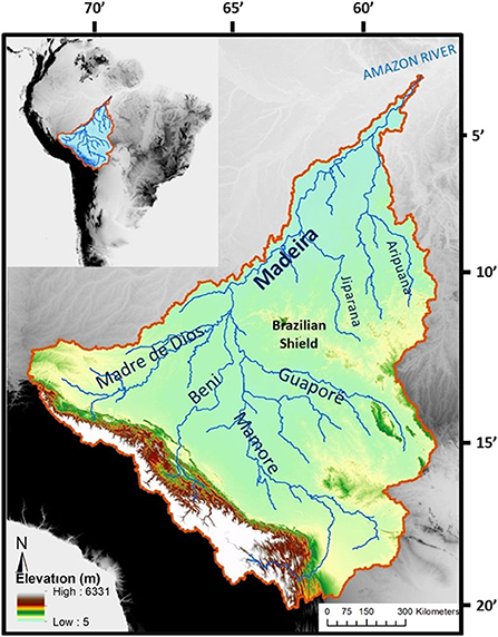
Figure 1. Location of the Madeira Basin (South America) and its main tributaries (blue lines) and topography (m).
The mean annual rainfall over the Madeira lowlands ranges from 2,500 in the north to 1,000 mm in the south (Roche et al., 1991), whereas a substantial variability is observed in the Andes with rainfall ranging from 200 mm at high altitude to 6,000 mm at the eastern flank of the Andes (Espinoza et al., 2014). The Madeira Basin is characterized by a south tropical rainfall regime with a marked dry season during the austral winter and a wet season during the austral summer (Ronchail et al., 2005). Indeed, approximately 75% of the annual rainfall is recorded from December to March (Espinoza Villar et al., 2009). The wet season is related to the presence of the South America Monsoon system, which brings humidity from the Atlantic Ocean and the Amazon rainforest (Vera et al., 2006). Many studies showed that a small fraction of interannual rainfall variability in the Madeira Basin can be related to the El Niño Southern Oscillation (ENSO) in the Andean region (Garreaud et al., 2003) or to tropical or subtropical Atlantic sea surface temperature in the lowlands (Ronchail and Gallaire, 2006). In the Andean basins, El Niño years are usually linked to dry conditions, whereas La Niña years are often wet (Ronchail and Gallaire, 2006). Critical flooding frequently occurs in the basin with major events in 2003, 2007, 2008, and more recently in 2014 (Ovando et al., 2016). The 2005 drought affected the whole Madeira Basin (Marengo et al., 2008; Zeng et al., 2008).
3. The SWAT-floodplain model
SWAT is an agro-hydro-environmental model developed by the USDA Agricultural Research Service (USDA-ARS; Temple, TX, USA) and Texas A&M AgriLife Research (College Station, TX, USA; Arnold et al., 1998). It is a conceptual, semi-distributed, and physically based hydrologic model initially designed to predict the impact of human activities and agricultural management on water and sediment yields. The SWAT model is frequently used on the world's main rivers and its performance has already been evaluated at several catchment scales and in various pedoclimatic conditions (Faramarzi et al., 2013; Abbaspour et al., 2015; Krysanova and White, 2015; Du et al., 2018). The detailed functioning of the model is available online in the SWAT documentation (http://swatmodel.tamu.edu/). To our knowledge, this is the first study to showcase the SWAT model as the only core of a large-scale alluvial floodplain hydrodynamic framework delineated with remote-sensing observations. Our approach is constituted by a recently modified version of the SWAT where the water routing is performed by a hydraulic approach (Santini, 2020) and a redesigned floodplain module. The framework also involves remote sensing observations of water surface extents (e.g., floodplain delineation) as direct input data of the model. It handles large-scale areas with high-resolution stream networks and daily simulations.
3.1. Design of the floodplain module
In the default SWAT model, the floodplain width is linked to the morphology of the reach it is connected to. The floodplain width is defined as five times the width of the reach at bank full level. The floodplain acts as a larger reach during the inundation where the velocity of the water is calculated within the cross-section of both the river and the floodplain. The floodplain network in SWAT is disconnected which means that there is no water exchange from two consecutive downstream floodplains. These formalisms appeared unsatisfactory to represent sediment and nutrient dynamics in floodplains. Figure 2 depicts the general concept of the SWAT-FloodPlain model. The floodplain module of the framework offers a fully connected floodplain network. A floodplain entity is associated with a sub-basin and reach and lateral water exchanges can occur between the reach and its floodplain depending on the water volume/height in the reach and the floodplain, respectively. In the SWAT-FloodPlain model, we introduced two different floodplain functioning (i) a longitudinal flux of water can happen between the upstream and the downstream floodplain. In this case, the exchange is represented by a kinematic wave during flooding. (ii) The floodplain acts as a reservoir and only stores water during the flooding event. Furthermore, to address the Gauckler-Manning-Strickler representation, each floodplain is characterized by a calibrated Manning-like coefficient (see below) ranging from 0.02 to 0.15 s.m−1/3.
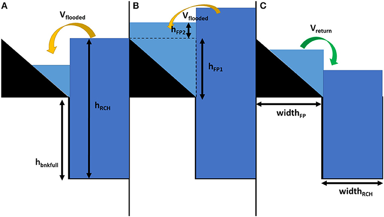
Figure 2. Simplified representation of the different processes of the overflowing and the return of water in SWAT-FloodPlain. The volume of water entering the floodplain is linked with the water height difference between the floodplain and the stream. hFP is the water height in the floodplain when (A) it is not saturated. In case (B), the water is stored vertically. (C) The water returns to the stream regarding the height in the stream and the floodplain.
This coefficient is also used to discriminate the functioning of the floodplains. In the study, we considered that floodplains with a Manning coefficient above 0.8 s.m−1/3 were modeled using case (ii).
In the SWAT-FloodPlain model, the continuity equation in the reach is:
with ΔVRCH is the water volume stored in the reach, Vin is incoming water volume, and Vout is outgoing water volume, Vflooded is the volume of water overflowed leaving the reach for the floodplain during flooding, and Vreturn is the water volume coming from the floodplain to the reach during downswing. In SWAF-FloodPlain, this equation is coupled with the continuity equation of the floodplain:
with ΔVFP is the water volume stored over the floodplain, VFPin is the incoming water volume in the floodplain; i.e., coming from the upstream, and VFPout is the outgoing water volume from the floodplain. Vflooded and Vreturn are defined as previously. All units are in m3.
Vflooded and Vreturn are the same in Equations (1) and (2). Fluxes exchange between the floodplain and the reach depend on the water height in the two reservoirs (Figure 2). During flood events, i.e., when the water height in the reach is superior to the water height at bank full level, the floodplain is active and can receive water from the stream and three cases occur.
• If the volume of water in the floodplain is superior to the maximal volume capacity of the floodplain (Figure 2B), the floodplain acts as saturated. Thus, even though the volume of water can still increase in the floodplain, its extent is constrained by the maximum width of the floodplain. The floodplain flow to the downstream floodplain is modeled as follow:
PFP the wetted perimeter of the floodplain (m), α is slope of the floodplain from the landside to the reach, widthFP is the width of the floodplain (m), and AFP is the wetted area (m2). UFP is the floodplain velocity calculated by the Gauckler-Manning-Strickler equation (m.s−1), S0 is the slope of the reach (m.m−1), and CHN3 can be apprehended as a manning's roughness coefficient of the floodplain (s.m−1/3). Furthermore, we introduced an average velocity UAV (m.s−1) between the reach and the floodplain to accurately represent the deceleration of the reach flow caused by the overflow in the floodplain. It is then used to calculate the respective flow discharge of the reach and the floodplain.
Where QRCH (QFP, respectively) is the water discharge in the reach (in the floodplain, respectively) in m3.s−1. Afterward, the model compares the water height in the reach and the floodplain to establish a possible lateral exchange from the floodplain to the reach.
Where hFP is the water height in the floodplain (m), VRCH (respectively, VFP) is the volume of water in the reach (respectively, in the floodplain) (m3), lrch is the length of the reach (m), and hbnkfull is the water height at bank full level (m). If hRCH < hbnkfull a fraction of the floodplain volume returns to the reach as
• When the floodplain is not entirely filled (Figure 2A) and hRCH > hbnkfull, the module calculates the amount of water transferred from the channel to the floodplain which depends on the water stored in the reach and the water height:
where VFPin is the volume of water leaving from the reach to the floodplain, VRCH is the volume of water in the reach, and lrch is the length of the reach. h'RCH is the solution of the water level in the reach as shown in Santini (2020). Then, the model updates the amount of water in the floodplain considering this new volume and calculates the new water height in the floodplain.
The floodplain flow to the downstream floodplain is modeled in this section as follows:
Again, in order to integrate the deceleration of the water induced by the flooding, we introduced an average velocity similar to equation (6, 7, 8).
• When the floodplain is not saturated (Figure 2C) and hRCH < hbnkfull, the module does not simulate any flooding from the reach to the floodplain. On the other hand, the water leaving the floodplain to reach (Vreturn) is modeled first. Second, as long as there is water in the floodplain section, it is routed to the next floodplain as detailed in the previous section.
3.2. Floodplain delineation
The morphology of the floodplain is a key point for modeling water routing in large-scale rivers, such as the Amazon and the Madeira Rivers, where the floodplain can store water for several weeks or months. Indeed in the default version of SWAT, the floodplain is defined as five times the width of the stream. Two different data are used to delineate the floodplains.
3.2.1. DEM based delineation
In the study, we used the 500 m spatial resolution DEM from the SRTM (Farr et al., 2007; Figure 3). We upscaled the 90 m SRTM data to 500 m to be consistent with the resolution of both floodplain delineation methodologies (see next sub-section). The delineation of the floodplain is based on the method of slope thresholds described in Rathjens et al. (2015). The SRTM DEM is a global topographic data set widely used in hydraulic simulations and geomorphologic characterization of the Amazon floodplains but these data are affected by vegetation cover, speckle, and stripe noise (Fassoni-Andrade et al., 2021). In first approximation, these data are adequate to delineate the floodplains in the SWAT model regarding the study area, the model discretisation, and the aim of simplifying the processes. The SWAT-FloodPlain model for the Madeira Basin considers 1,445 sub-basins unit catchments of 500 km2 on average. Figure 3 shows the floodplains delineation computed with DEM data.
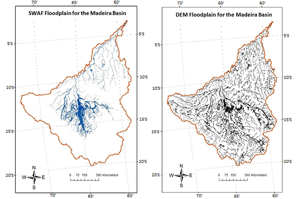
Figure 3. Spatial representation of the SWAF-HR floodplain (left) and the DEM-based floodplain for the Madeira Basin (right).
3.2.2. SWAF-HR based delineation
The fot Soil Water Fraction at High Resolution (SWAF-HR) data is used to determine the floodplain delineation in this study. The SWAF data is obtained using a contextual model on the SMOS brightness temperature. Soil Moisture and Ocean Salinity (SMOS) was launched in November 2009 by the European Space Agency (ESA) and was especially designed to map soil moisture over the globe every 3 days. SMOS is a passive microwave 2-D interferometric radiometer operating in L-band (1.14 GHz, 21 cm wavelength; Kerr et al., 2010). It provides brightness temperature (TB) emitted from the Earth over a range of incidence angles (0° to 55°) with a spatial resolution between 35 and 50 km. Parrens et al. (2017) and Fatras et al. (2021) showed the capability of SMOS to retrieve water surface fraction (e.g., inland bodies, wetlands, floodplains, lakes, rivers) under dense forests over tropical areas. A global-scale SWAF (GSWAF) was introduced in Al Bitar et al. (2020). Moreover, SMOS can measure Earth emission in all-weather conditions (even during heavy precipitation and cloudy sky). SWAF data provide water surface fraction over the Amazon Basin from 2010 to date each week over lowlands but it is not available over mountainous areas. Data are projected in the EASE-grid (approximatively 25 km). SWAF-HR data is a spatial desegregation of the SWAF data at 1 km (Parrens et al., 2019, Figure 3). The desegregation was performed by merging SWAF data, optical data (Global Surface Water Occurrence, Pekel et al., 2016), and radar data (Multi-Error-Removed-Improved-Terrain, Yamazaki et al., 2017). SWAF-HR data also provides the probability of a pixel being inundated. Pixels with a probability of inundation higher than 1% are decreed as belonging to the floodplain.
Once the floodplains are delineated for the whole stream network, the area of each landscape unit is then re-attributed to the corresponding sub-basin following the standard SWAT delineation procedure. In the model, the floodplain is associated with a reach and is assimilated to a prism with a triangular cross-section on each side of the reach where α is the slope of the floodplain and widthFP is the width of the floodplain (m). In this study, SWAT is computed twice, one with the floodplain delineated with DEM (SWAT-FP) and one with the floodplain delineated with SWAF-HR (SWAT-SWAF) allowing to evaluate the role of this delineation.
3.3. Precipitation forcing
Both SWAF-FP and SWAF-SWAT were forced with the TRMM-3B42 (Huffman et al., 2007) 0.25° spatial resolution daily precipitations between 2008 and 2019. These data are adequate for our study since Buarque et al. (2011) found that TRMM and rain gauges mean annual rainfalls were fairly similar over Brazil and Paiva et al. (2011) have shown the decrease of precipitation over large water bodies in the Brazilian Amazon with TRMM. The daily average precipitation over the Madeira basin is represented in Figure 4.
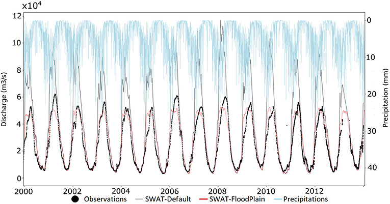
Figure 4. Comparison of simulated discharges for the default SWAT version (gray line) and the SWAT-FloodPlain (red line) at the Fazenda gauging station (−4.890;−60.026). The observations are displayed in black. The blue line represents the daily precipitations averaged over the whole watershed. For both simulations, parameters are run as follows: GW_DELAY = 80.00, ALPHA_BF = 1.00, GWQMIN = 1,000, REVAPMN = 1,000, GW_REVAP = 0.20, OV_N = 0.10, and CANMX = 200 and run with (Strauch and Volk, 2013), ESCO = 0.95, EPCO = 1.00, EVAPOT = 10.00, and Curve Number (CN) were calibrated by sub-basin.
The daily minimum and maximum temperatures from the ERA-Interim are used in this study (Berrisford et al., 2011).
4. Validation data and procedure
4.1. In situ data from the HyBAm observatory
In situ river data were obtained from the Critical Zone Observatory HyBAm (Hydrologie du Bassin Amazonien), a long-term monitoring program that is maintaining, in collaboration with the national stakeholders and local universities, 35 gauging stations in the Amazon catchment since 2003. For the Brazilian part of the Basin, a network of eight local stations is handled by the French National Research Institute for Sustainable Development (IRD) and the Federal University of Amazonas (UFAM). For the Bolivian part, the network is managed by the Bolivian hydrological service (SENAMHI) with the IRD and La Paz University (UMSA). All data are available at http://www.so-hybam.org for each gauging station over the Madeira Basin. Gauging stations from the Brazilian National Water Agency (ANA) were also used. In this study, the daily river water discharge and water stage for 18 stations were extracted and compared to SWAT simulations.
4.2. Spatial altimetry
The current spatial altimetry landscape regroups the ongoing missions CRYOSAT (2010), Saral (2013), Jason-3 (2016), Sentinel - 3A (2016), Sentinel - 3B (2018), CFOSAT (2018), HY-2B (2018), HY-2C (2020), and Jason-CS/Sentinel 6 (2020). TOPEX/Poséidon (1992–2006) was the first mission to apply spatial altimetry to inland waters (lakes, rivers, and floodplains) (de Oliveira Campos et al., 2001; Kouraev et al., 2004). Because of its all-weather capability and its ability to detect water beneath vegetation, radar altimetry became an essential tool for large-scale continental hydrology of ungauged areas (Birkett et al., 2002; Getirana et al., 2010; Hall et al., 2011; Frappart et al., 2018). However, the major limitations of spaceborne altimetry are its spatially limited measurements (where the river/lake/floodplain crosses the ground track of the satellite). In this study, we used the data of Jason-2 (2009–2017) and Jason-3 (2017–2019) over the tracks number 63, 76, 102, 139, 178, 241, and 254. Water height time series were calculated and extracted using the ICE-1 retracking of radar echoes (Frappart et al., 2006; Calmant et al., 2013). In order to specifically focus on the floodplains, we applied a filter on the backscattering values of the series and selected only data with a backscattering value above 20 dB. Indeed, backscattering is a proxy of what is measured by the satellite. Water bodies usually have a high signature in terms of backscattering coefficient. In the case of floodplains, where the area alternates between wet and dry conditions, we considered that the flooding occurs for backscattering values at 20 dB (Martinez and Le Toan, 2007; Frappart et al., 2020). Considering that floodplains are inundated only part of the year, we assumed that getting low signals during the low water period was irrelevant. This helps to remove outliers and artifacts that might have been recorded after heavy precipitations.
4.3. Validation of the water surface dynamic in floodplains with altimetry
This section presents the methodology leading to validate the simulated volumes of water in floodplains with spatial altimetry. The objective is to compare the water height extracted from spatial altimetry with the water height calculated by the model (based on the simulated volumes) in floodplains. Once the model was calibrated and validated with the gauging stations on the discharge in the rivers, the floodplains were calibrated where altimetry tracks were available. The objective was to determine an optimal couple of latitude and floodplain Manning coefficient (CHN3 see Section 3.1) for a floodplain section. To achieve it, the model was run with it ranging from CHN3 0.02 to 0.15 s.m−1/3 with a step of 0.01. The water height in the floodplain was then compared to the altimetry water height time series. In the framework, the floodplain is assimilated as two triangles. The average floodplain width is either determined by SWAF-HR or by the DEM, α is the floodplain slope to the river, and the water height is retrieved with altimeters. In this configuration, the water height depends on the volume of water in the floodplain and the distance to the river. As so, comparing the water heights from the model and the altimeter requires the exact position of the sampling point of the satellite. The location of the reflective surface (generally the water body) as seen by the sensor is often imprecise which can induce errors in the estimation of the volume. Nevertheless, in the Madeira Basin, the slope of the floodplain is very low (α between [0.03%, 0.06%]). Thus, the geometry of the floodplain can be assimilated as two rectangles. Therefore, in this configuration, the water height measured with the altimeter can be compared to the water height extracted from the model as it only depends on the volume in the floodplain. Overall, the main hypotheses we make are that the water height in the floodplain is a linear relationship to the water volume in the floodplain and that validating the water heights simulated by the model with water heights measured with altimeters is equivalent to validating the water volumes. Yet, determining the localization of the measuring point of the altimeter stays critically essential. It needs to satisfy some requirements: it shall represent only the hydrodynamics of the floodplain not the stream or others nearby water bodies. The location of the point shall be robust and not change throughout the period. Therefore, in the best scenario, the location of the measuring point should be in an alluvial floodplain, far enough from the stream to avoid any signal contamination, and it should detect no water during the low water period but should get a signal as soon as the flood episode starts. To meet all the specifications and to avoid any user dependency, we designed a qualitative algorithm to properly place the measuring point of the altimeter. The objective here was to determine the latitude where the measuring point should be set for a satellite track and a sub-basin. First, we used the SWAF-HR overlay alongside the ground tracks of the satellites and the SWAT sub-basins to determine the areas that were likely to be flooded. Afterward, we compared the theoretical stream network simulated by SWAT with the existing stream network delivered by aerial or spatial imagery such as those found on Google Earth or on other web map servers. It allowed us to discriminate the sub-basins and the areas for our analysis. Second, for a designated track and sub-basin, we extracted the backscattering values over the range of the SWAF-HR overlay. The backscattering indicates the reflectivity of the surface at the nadir of the satellite and is therefore a valuable indicator of the nature of the object measured by the satellite. We considered that points with a backscattering value of over 20 dB were inundated at least part of the year. Thus, this gave us a minimum and maximum latitude for each floodplain section on where to run our analysis. Finally, for each latitude between the minimum and maximum latitude, with a step of 0.02°, we extracted the water height series from the altimeter and compared it to the water height series simulated by the model. For the comparison, we normalized both series to avoid any bias induced by the geoid or the DEM used in the simulation. Three indexes were calculated for each comparison: the Pearson's correlation index, the percentage of bias (pbias), and the root mean squared error (RMSE). The measuring point was set up on the latitude where the three indicators were optimal for the best floodplain Manning run.
5. Results
5.1. Discharge
Figure 4 shows the difference in discharge simulation for the default SWAT version and the SWAT-FloodPlain at the outlet gauging station of the Madeira (Fazenda gauging station). Each simulation was run with the same set of parameters. First, for discharge, SWAT-FP and SWAT-SWAF appear to simulate very close value as displayed as a red line. Second, the floodplain module significantly improves the discharge in the reach. Indeed R2 and NSE for SWAT default are about 0.91 and −0.23, respectively, while R2 and NSE index for the SWAT-FloodPlain module are 0.94 and 0.89, respectively.
5.2. Evaluation of the floodplain extent for SWAT-FP and SWAF-SWAF
Table 1 exposes the frequencies of the floodplain areas for the SWAF framework. From the 1,445 sub-basins that constitute the Madeira Basin, only 781 sub-basins display a floodplain. In total, the floodplain estimated by SWAF-HR represents an area of 86,587 km2 with an average area of 59 km2 per sub-basin. The distribution of the floodplains is centered around small areas where 62% of the sub-basins have a floodplain area under 70 km2. The SWAT-FP framework has a theoretical floodplain delineation. As so, all sub-basins have a floodable section. The cumulated floodplain area for that delineation methodology is 205,159 km2 with an average area of 141 km2 per sub-basin. The distribution of the areas for the DEM methodology is more homogeneous than for SWAF-HR. Indeed, only 32% of the sub-basins have an area under 62 km2, 27% have a floodplain area between 62 and 126 km2 while 25% of the sub-basins have an area of floodplain superior to 189 km2. SWAF data are only available in the lowlands. So, we extracted the area of the DEM methodology on the same sub-basins where SWAF was available. As so, it appears that the DEM areas are on average larger that the SWAFs for the same sub-basins; with a difference of 110 km2 on average. Moreover, in spite of the SWAF product been not available in mountainous areas, these represent almost half of the floodable areas for the DEM methodology. Thus, they constitute a non-negligible factor when estimating the inundations. Hamilton et al. (2002) found that the maximum of area subject to flooding in a calendar year over the Llanos de Moxos (the most important Madeira floodplain) is equal to 92,090 km2, whereas the mean area flooded during the 1967–1997 period is equal to 29,460 km2. Paiva et al. (2013) estimated with the MGB-IPH model that the maximum of the Bolivian floodplain is equal to 20,000 km2, whereas an estimation of 80,000 km2 has been found by using satellite data (GIEMS). Next, on the sub-basins that presented a SWAF-HR floodplain, the difference between the DEM methodology and SWAF-HR was calculated. Figure 5 represents the histogram of the results. A total of 76% of the sub-basins shows a positive difference indicating that in most cases, SWAF-HR underestimates the floodplain area compared to the DEM methodology. The main peak is for the basins where the difference is between 0 and 20 km2 and corresponds to 12% of the sample, 32% of the basins show a difference smaller than 50 km2 while half of the differences between the two methodologies are under 100 km2. On the other hand, only 17% of the area differences are between 0 and −100 km2.
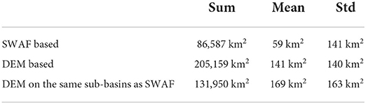
Table 1. Floodable areas for the different floodplain delineation methodologies (SWAF and DEM based) and the area estimated by the DEM based methodology on the sub-basins where SWAF data is available.
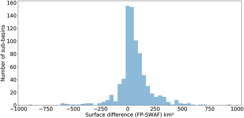
Figure 5. Distribution of the areas of the estimated floodplains for the SWAF and DEM methods. If the value is positive, then the DEM methodology estimates a larger floodplain than SWAF. Overall both methods return similar floodplain delineations.
5.3. Surface water storage
Figure 6 presents the interannual average variations of the floodplain surface water cycle over the Madeira Basin for SWAT-SWAF and SWAF-FP. The maximum of floodplain water storage is reached at the beginning of March for the two frameworks. This result is in accordance with Frappart et al. (2012), where the authors estimated the surface water storage of the Madeira Basin of about 800 to 1,000 km3 per year between 2003 and 2007. Even though the period of their study and ours do not coincide, their estimation and our modeling return close values. On average, the amount of water stored in the floodplain is about 810 ± 230 km3 per year for SWAT-SWAF and 1,300 ± 350 km3 per year for SWAT-FP. The two models return a difference of about 490 km3 per year in the estimation of the volume of water in the floodplains. This difference comes from the fact that the DEM estimation of floodplains assesses more uplands as floodplains than SWAF-HR. The estimation of the volume by SWAT-FP on the same basins where SWAF is available returns an average volume of 1,032 ± 270 km3 per year. Nevertheless, SWAT-SWAF outputs cover 85,587 km2 and are responsible for more than 62% of the surface water storage of the whole Madeira Basin. Moreover, the rest of the floodplains, which cover 118,572 km2 and are located in upland areas or on small streams, may participate to one-third of the storage capacity of the Madeira Basin.
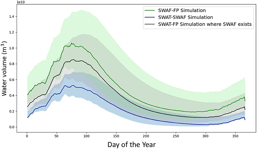
Figure 6. Average daily water storage in the floodplains of the Madeira Basin for the SWAT-FP model (green), the SWAT-SWAF model (blue). The gray color refers to the extraction of the volumes for the SWAT-FP model on the locations where SWAF exists.
5.4. Comparison of the simulated water heights with altimetry
Performance of the models SWAT-SWAF and SWAT-FP were estimated on 64 validating points over the Madeira Basin. Figure 7 shows time series of standardized simulated water heights for the SWAT-SWAF and SWAT-FP models compared to Jason-2 and Jason-3 standardized water heights over the period 2008–2019. The upper part of the figure displays the comparison with the SWAT-SWAF model while the lower part of the figure displays the comparison with the SWAT-FP model. The left-hand side represents cases of particularly good correlations between the simulations and the observations whereas the right side shows low to satisfactory correlations. The models succeeded in reproducing the variety of water dynamics in the floodplains: from floodplains where the inundation is recurrent to floodplains where the inundation presents no pattern. For example, the left graphs in Figure 7 show a floodplain where the inundation pattern looks steady. Nevertheless, in 2016, both models simulate an inundation that appears to be less intense than the previous years. Indeed, the peak is shorter and thinner for this year. This episode is corroborated by both altimeters Jason-2 and Jason-3 where the amplitude of the measurements is shorter, and the dispersion of the points is more centered.
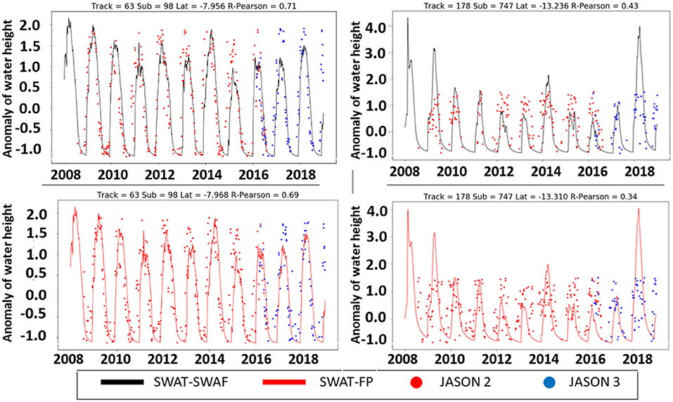
Figure 7. Comparison of water height variations in the floodplain between the SWAT-SWAF/SWAT-FP framework and altimetry data from 2008 to 2018. The dots refer to measurements of anomalies of water height from altimeters Jason 2 (red) and Jason 3 (blue) in floodplains. The lines represent the simulated anomalies of water height in floodplains from the SWAT-SWAF framework (black) and SWAT-FP (red).
On the one hand, for the SWAT-SWAF model, the mean value of the R-Pearson for the 64 series is 0.49 ± 0.18. The maximal and minimum values are equal to 0.84 and 0.17, respectively. On the other hand, the time series with the SWAT-FP framework presents a mean value of equal to 0.52 ± 0.18, with a maximal value of 0.87 and a minimum value of 0.18. Overall, both models present a satisfactory to good capacity to represent the variations of the water height in the floodplain compartment. To evaluate the performance of the two models, we compared the values of the different indexes for SWAT-SWAF and SWAT-FP at each validating point. Figure 8 exposes the histograms of the different indexes for both models. Both frameworks present satisfactory unbiased simulated values. For the SWAT-SWAF model, the mean p-bias value is 88.6 and 93.0% of the points are between −49.0 and 173.0. For the SWAT-FP model, the mean value for the p-bias is 92.5 while 92.0% of the points are between −121.0 and 280.0. The repartition of the values of the p-bias for both models is similar even though there are two to three points for each model that present particularly high negative indexes. On the one hand, for the SWAT-SWAF model, 47.0% of the sample presents a correlation superior to 0.50, and 63.0% of the points have an index superior to 0.40. On the other hand, for the SWAT-FP model, 52% of the points show an R-Pearson above 0.50 and 70% show a correlation over 0.40. Even though the SWAT-FP model seems to have an overall better correlation than the SWAT-SWAF framework, the R-Pearson histogram displays a similar distribution of the index for both models. It tends to indicate that both frameworks are equivalent in terms of performance. To confirm that statement, we ran an Analysis of Variance (ANOVA) on our samples. The analysis returned a p value of 0.42 implying there is no statistical difference in the use of both models.
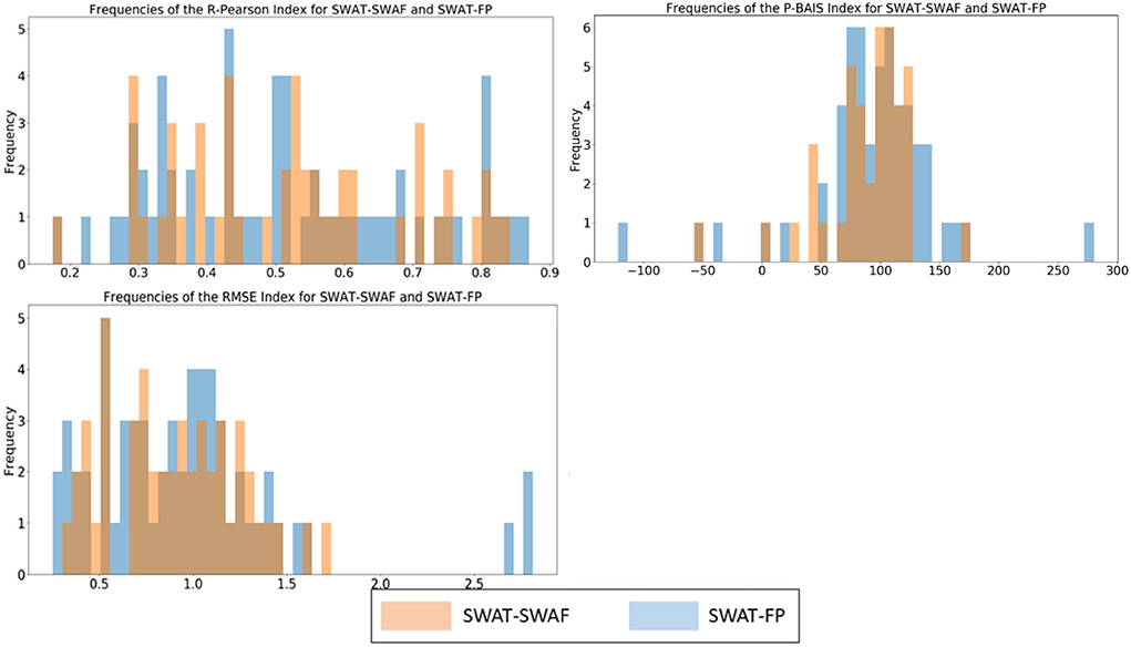
Figure 8. Histograms of the R-Pearson, p-bias, and RMSE indexes for both frameworks.
For the SWAT-SWAF model, the mean RMSE is 1.21 with a SD equal to 0.91 and 62.0% of the sample shows a value inferior at 1.21. For the SWAT-FP framework, the mean RMSE is 1.08 ± 0.77 and 60.0% of the points have an RMSE below 1.08. The RMSE histogram indicates that the distribution of the index is similar for the two models despite some small differences. Indeed, the SWAT-SWAF framework presents a high frequency of points at 0.5 while the SWAT-FP shows a high frequency of points around 1.00 and four samples above 2.00. Nevertheless, it appears that the performance of the models for the RMSE index is equivalent (Kruskal-Wallis test, p = 0.25). Figure 9 represents each point and the R-Pearson and the RMSE index, the best model between the SWAT-SWAF and SWAT-FP frameworks. For the R-Pearson, most of the points are covered by the SWAT-FP model, whereas it is the opposite for the RMSE index where most of the points refer to the SWAT-SWAF model.
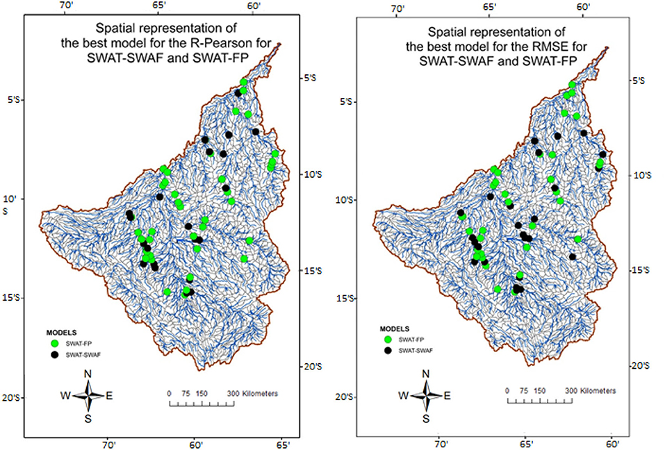
Figure 9. Spatial representation of the best framework on each validation point for the R-Pearson index (left) and the RMSE index (right). Green dots mean that the index is better for SWAT-FP while black dots correspond to SWAT-SWAF. Both models appear close in term of quality.
5.5. Comparison of the SWAT-SWAF and SWAT-FP with the dynamics of the floodplains
In Figure 10, we classify our two models depending on features observed in the comparison of the variations of the water height in the floodplains for the SWAT-FP and the SWAT-SWAF models. Ten groups are identified. The left side of the figure exposed the spatial location of the different groups. Table 2 presents the number of sub-basins belonging to each group. Group 4 is in the majority with 28 sub-basins. Group 7 and 9 only contain two sub-basins each.
• Group 1 is constituted of three sub-basins where the variations of the SWAT-FP model are higher than the SWAT-SWAF model. Moreover, this group is characterized by a recession of the water in the floodplain occurring earlier in the SWAT-FP model.
• Group 2 is constituted of four sub-basins where the variations of the two models are similar. Nevertheless, flooding for the SWAT-FP framework occurs slightly earlier (less than 10 days) than for the SWAT-SWAF model.
• Group 3 is constituted of four sub-basins. The group is characterized by greater variation of the SWAT-SWAF model than the SWAT-FP model.
• Group 4 is constituted of 28 sub-basins. The group is characterized by variations of the water height in the floodplain almost identical for both models.
• Group 5 is constituted of six sub-basins. The critical point for the group is that some floods are simulated in the SWAT-FP model and are not present in the SWAT-SWAF model.
• Group 6 is constituted of four sub-basins where the variations of the SWAT-SWAF model are higher than the SWAT-FP model. Moreover, this group is characterized by a recession of the water in the floodplain occurring earlier for the SWAT-SWAF model.
• Group 7 is constituted of two sub-basins. It is the opposite of the previous group where in this case, the variations of the SWAT-FP model are higher than the SWAT-SWAF model. Moreover, this group is characterized by a recession of the water in the floodplain occurring earlier for the SWAT-FP model.
• Group 8 is constituted of five sub-basins. It is a peculiar group where the dynamic of the variations of the water height in the floodplain is different between the two models.
• Group 9 is constituted of two sub-basins where the variations of the SWAT-FP model are higher than the SWAT-SWAF model. Nevertheless, flooding for the SWAT-SWAF framework occurs earlier than the SWAT-FP model and tends to last longer.
• Group 10 is constituted of three sub-basins. For most years, the variations of the SWAT-SWAF are higher than the SWAT-FP model in this group. The tendency shifts in 2008, 2009, 2014, and 2018 where the variations of water height in the floodplain for the SWAT-FP model are greater. Those years correspond to significant floods over the Madeira Basin.
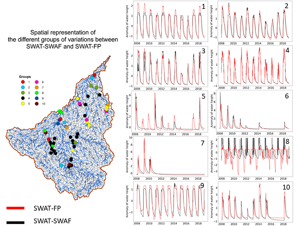
Figure 10. (Left) Spatial representation of the different groups identified. Each color represents a unique group. (Right) Graphic description of the different groups identified regarding the variations of water height in floodplains between the two frameworks.
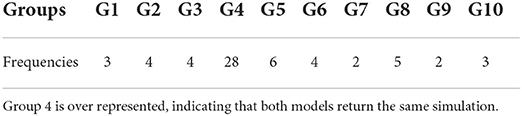
Table 2. Frequencies of the different groups identified in the functioning of the floodplains.
These 10 groups were built regarding the results of the simulation. We could have regrouped some of them but, they show different functioning of floodplain and emphasize the importance of the delineation of the floodplain.
5.6. Effect of the floodplain delineation methodology on the performance of the model and the different groups
The comparison between the observed variations of water heights in the floodplains and the ones simulated by the two frameworks highlighted no statistical differences in general. Yet, delineating the floodplain area constitutes a key point in the model. Both frameworks present a peculiar methodology to estimate the floodplain area within a sub-basin in the SWAT model, which can lead to a local difference in the modeling. While the SWAF-HR methodology is based on remote-sensing observations and is not available on the whole Madeira Basin (mountainous areas are not included in the SWAF data), the DEM methodology concerns all the sub-basins. Therefore, it appears that, on average, for a given sub-basin, the cumulative floodplain area of the drainage area for the DEM delineation is always higher than for SWAF-HR (Figure 5). Figure 11 represents the floodable area estimated by SWAF-HR in function of the floodable area computed with the DEM methodology. Each dot corresponds to a sub-basin where the color depicts the location of the basin in the Madeira watershed. A low index (represented by red dots) means that the basins are located near the outlet of the watershed and on the main stem of the Madeira River. On the contrary, basins with an index between 600 and 1,000 (green/blue dots) are located in the Bolivian floodplain of the watershed. In both charts, the black line corresponds to the first bisecting line (Δ) and the green line (R) corresponds to the best polynomial regression between the FP area and the SWAF-HR area (polynomial of order two). First, most sub-basins are above the first bisecting line indicating that either the FP area is over-estimated or the SWAF-HR area is under-estimated, and it covers all location indexes. Nevertheless, sub-basins that possess a particular high location index, above 1,200 and dark blue shade, are the only category where the SWAF-HR area is systematically under-estimated. Indeed, these basins have a DEM based FP area of more than 100 km2 but an estimation of the SWAF-HR area under 10 km2. As a matter of fact, they correspond to the limit for the detection of SWAF-HR toward upland and mountainous areas. Overall, all basins regardless of their position in the watershed are subjected to an over/under estimation by both methodologies. However, it appears that there is a pattern in how the sub-basins scatter. In fact, most of the low-index basins are located on the left-hand side of the point where Δ and R cross, while most of the middle-index basins are on the right-hand side of that point. The high-index basins seem to scatter around to above R. Overall, this chart is an indicator of the distribution and the topography of the floodplains in the Madeira Basin. Most narrow floodplains are located near the outlet of the watershed, alongside the main stem of the Madeira River and its eastern tributaries and the Madre Dos Dios River. These floodplains are usually understated by SWAF-HR. On the contrary, large floodplains are located in the flat Bolivian part of the watershed and alongside the Guapore River. Figures 11A,B focus on the points considered in the study. In Figure 11A, the points are colored regarding their group while in Figure 11B, the color panel represents their location in the watershed as emphasized previously. First, it appears that the groups scatter according to a proper pattern. On the one hand, groups 1 and 8 are located close to Δ while groups 3 and 10 are on the R line. On the other hand, these sub-basins do not have a specific location in the watershed: the index of these points varies from low to high. Moreover, these groups do not share any common features. As a matter of fact, group 1 is characterized by the inundation occurring slightly earlier for SWAT-FP than for SWAT-SWAF, but it is the other way around for group 3, while group 8 has no feature. As so, the differences in the dynamics of the variations of the water height in the floodplain appear to be an inherent property of the framework used. This fact is emphasized in group 4. Indeed, these sub-basins are scattered mostly between the Δ and R curves and are located throughout the Madeira watershed. Yet, group 4 is characterized by both models returning a similar response for the water dynamic in the floodplain. Nevertheless, all the groups discussed above share a common topographic feature. Indeed, they are all located either on main stems or on sections where the cumulative area of the floodplain of the drainage area (especially for the SWAT framework) is superior to 50 km2. First, this implies that the floodplain dimension does not highly constrain the inundation. Second, it means that inundations may have had occurred in upstream basins and the flood pulse may have been propagating through the stream network. It is therefore a key point in the modeling of flooding. Indeed, groups 5, 6, and 7 are located on the extreme left-hand side of the charts where the estimation of the floodplain by the DEM methodology is usually ten times wider than SWAF-HR. Moreover, these basins are located in the eastern part of the lower Madeira watershed, on tributaries and relatively small streams. Group 5 is characterized by the fact that some floods are simulated in the SWAT-FP model and are not present in the SWAT-SWAF model. In the meantime, these basins are the first basins in the network with a SWAF-HR floodplain. Moreover, these are areas in the limits of the SMOS sensors. Thus, for that case, the flooding is limited by the floodplain delineation and does not take into account up-stream processes. Groups 6 and 7 share the same area features but with a higher estimation of the SWAF area for group 6. Group 6 is characterized by the inundation occurring slightly earlier for SWAT-SWAF than for SWAT-FP, and it is the opposite for group 6. Overall, for these peculiar basins, the floodplain plays a critical role in the temporality of the inundation as it specifically impacts the velocity of the water in the floodplain section. Overall, a correct delineation of the floodplain is paramount in the framework. It is especially the case for headwater basins and small streams.
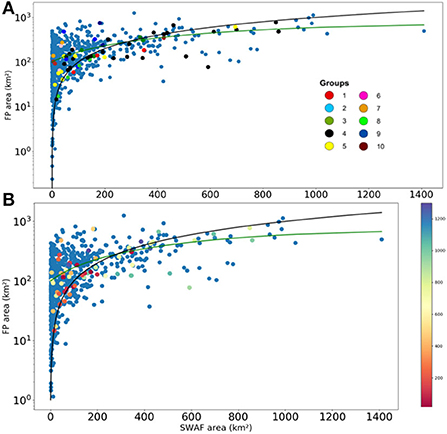
Figure 11. Relationship between the floodplain areas of the DEM delineation and the SWAF-HR estimation for each sub-basin. The index represents the location of the sub-basin in the watershed. A low index refers to a sub-basin located near the mouth whereas a high index means the sub-basin is in headwaters. (A) Specific focus on the groups. (B) Location of the specific sub-basins. It appears that most ‘group' sub-basins are located between the first bisecting line (black line) and the best polynomial regression (green line).
6. Discussion
6.1. Impact of the floodplain delineation
At a local scale, the two models (SWAT-FP and SWAT-SWAF) have similar temporal behavior. This result is proved by the similar statistics obtained in Figure 6. While the two models differ by the amount of freshwater estimated at the global scale, they return close results at the local scale of sub-basins (Figure 7). On average, SWAT-FP estimates 50% more freshwater storage in the Madeira Basin than SWAT-SWAF (Figure 5). This difference is explained by the lack of SWAF-HR data over the mountainous areas, covering 62% of the Madeira Basin. Comparison and validation of the two frameworks at the scale of the Madeira Basin are extremely difficult because the dynamic of the freshwater storage over this basin has not been estimated to our knowledge. Only, few studies, such as Frappart et al. (2012), explore the variation of freshwater storage over the Madeira Basin in order to detect extreme events (drought or floods) but no absolute value of water surface storage has been evocated. Other studies have worked at the scale of the Amazon Basin (Richey et al., 2002; Papa and Frappart, 2021) leading comparisons impossible. Some punctual comparisons are possible: (1) in 2014, a massive flood was observed over the Madeira Basin. Ovando et al. (2018) found that for the Mamore floodplains that constitute the large Bolivian system, the surface volume of water stored ranged from 10 to 94 km3, the latter having been observed during the peak of the event. In 2014, we found that for SWAT-SWAF, the surface volume of water in the Mamore floodplains ranges from 15 to 240 km3. For SWAT-FP, the estimation varies from 54 to 418 km3. (2) For the whole Madeira Basin, Tourian et al. (2018) estimated a surface water storage of about 360 ± 10 km3. Nevertheless, the scare resolution and the sensors used in both studies are highly likely to underestimate the surface extent of water bodies and thus the estimation of surface volumes. As a reminder, we found that the amount of water stored in the floodplain is between 810 ± 230 km3 (SWAT-SWAF) and 1,300 ± 350 km3 (SWAT-FP). The range of these results is higher than the latest studies cited before. The floodplain delineation plays a key role in the global estimation of the Madeira floodplain storage. The need for a better characterization of the water surfaces over a tropical area at high spatial resolution is crucial to improve our estimation.
6.2. Effects of parametrization on the flooding
In the model description, three variables are critical for the flooding and the estimation of the volumes in the floodplains: the bank full level (hbkfull), the slope of the floodplain from the upland to the river (α), and the coefficient of Manning in the floodplain (CHN3). Bank full level represents the water level in the river at which the inundation is triggered. This parameter is of high significance to determine the moment and the intensity of the flooding. In SWAT-FloodPlain, the morphology of the cross-section of a channel is assimilated as a rectangle. The dimension of the channel, width, and depth, is calculated through the HydroTools processes and is averaged for each sub-basin. In the model, bank full level is defined as the elevation of the highest surface, i.e., when the water level in the channel reaches the maximum elevation. Estimation of bank full level is highly dependent on the DEM resolution. It plays a crucial role in regulating the temporality and the amount of water flooded. Therefore, as bank full level is a parameter of high significance that drives and constrains most of the flooding process, proper river geomorphology estimation through the DEM is a key point for flood modeling. On the same level, the angle of the floodplain α that characterizes the slope of the upland areas toward the river is the driver of the flooding. Indeed, as explained in $4.3, α mainly constrains both the water level and its expansion in the floodplain. Thus, to apply appropriately the methodology designed for alluvial altimetry, accurate estimations of the floodplain slope is required. In the case of the Madeira Basin, the floodplain slopes are almost flat which influenced little the estimation of simulated water height in the floodplain. But again, a good DEM resolution is the key point. Figure 12 describes the results obtained for the SWAT-SWAF on the anomaly of simulated water height with different Manning coefficients set in the floodplain. First, this shows the impact of the Manning coefficient in the floodplain. CHN3 in the SWAT-FloodPlain model modifies both the temporality and the water height (thus the volume) in the floodplain. Estimating this coefficient with precision is therefore critical for assessing the dynamic and estimating the volume of water in the floodplains. Second, the results of this analysis establish the possibility of using spatial altimetry applied to floodplains in order to calibrate at least the Manning parameter from the floodplain module of the SWAT-FloodPlain model. Indeed, by discriminating the Manning values in the floodplain, this comparison indirectly validates the velocity of the flow in the compartment and the effect of vegetation.
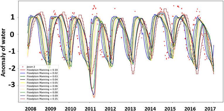
Figure 12. Comparison of the different Manning coefficients in the floodplain and the anomaly of water height time series for Jason 2 (red dots). Each color represents a different Manning coefficient for the floodplain leading to different velocity and a different magnitude of the flooding. This is extracted from sub-basin n°295 under track n°241 at the latitude −10.148.
6.3. Appropriateness of using spatial altimetry in floodplains
In this section, we classified each validation point regarding if the altimeter crosses the river, the floodplain, or the section in-between. To do so, we considered that if the river crosses or occupies most of the footprint, the point was classified as “river”. When the river was close to the edge of the footprint or when a hydrologic target was less than 200 m away, the point was classified as “between” as both the river and the floodplain contribute to the signal. Finally, “floodplain” points are represented by a footprint far from the influence of the river. Figure 13 shows the distribution and classification of each point for each framework. For the SWAT-FP model, 45% of the points are classified as “river”, 38% are floodplain points. For the SWAT-SWAF, 38% of the points are river points while 42% are floodplain points. Overall, the proportion of river and floodplain points for the two frameworks is equivalent. Most of the river points are located on the main stem of the Madeira and usually the river points denote a ratio between the area/width of the floodplain and the area/width of the stream inferior to 1. This infers that, for those cases, conventional altimeters do not have to capability and the resolution to distinguish the river from the floodplain. We investigated the impact of the type of validation points on the performance of the modeling for each framework. All tests (Kruskal-Wallis and ANOVA) systematically returned p values above 0.36. Thus, the type of virtual station has no significant effect on the quality of the modeling. Conventional altimeters were originally designed to monitor first the oceans and then were used in terrestrial hydrology with several applications on rivers and lakes water height. Our results tend to indicate that conventional altimeters as Jason-2 and Jason-3 can further be used to monitor altitudes on unusual hydrologic targets, such as alluvial floodplains in large-scale watersheds.
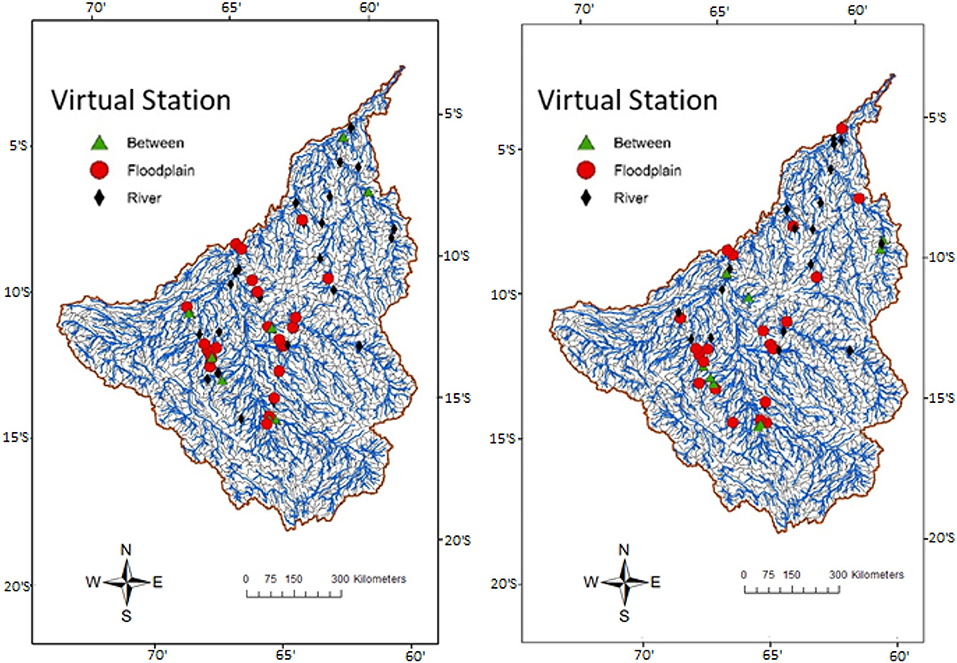
Figure 13. Location of the classified virtual stations for the different frameworks. A black diamond means that the virtual station (VS) is located on a river, while red dots mean that the VS is located in a floodplain where the altimeter is not influenced by the river. A green triangle means that the VS is located on land but close enough to the river for the signal to be influenced.
Furthermore, we compared how the same validation points were classified between the two frameworks. Most of the points (70%) are evenly classified in both models. Usually, if there is a different classification, it concerns points that transition from river to “between” or the other way around and points that were classified as floodplain in one model and “between” in the other. Only less than 5% of the points are classified as river in one model but as floodplain in the other model (or the other way around). This result indicates the robustness and the consistency of the altimetric measurement as well as the relevance of using altimetry data in alluvial floodplain to validate inundation module of models. Indeed, it shows that regardless of the frameworks used, a validation point usually refers to a unique hydrological component, either the river or the floodplain, and is unlikely to switch between them. Moreover, this opens possibilities to use altimetry data to improve the understanding of the dynamic and the functioning of alluvial floodplains. Indeed, a river point indicates that the dynamic of the floodplain is highly influenced and controlled by its connected stream while a floodplain point suggests that the mechanism of the inundation is complex and multi-factored.
7. Conclusion
This study presents a new floodplain module for the SWAT model with two different methodologies to delineate the floodplain with the aim to better characterize the hydrology of Madeira floodplains. In the SWAT-FloodPlain model, the floodplains are connected, allowing a transfer of water between the stream and the floodplain and between two consecutive up and down stream floodplains. The propagation of the flood pulse in both the stream and the floodplain is apprehended using a kinetic wave. We also designed a methodology based on the use of conventional spatial altimetry (Jason-2 and Jason-3) in alluvial floodplains to validate the floodplain module. The results show first the capability of using conventional altimetry over unusual terrestrial areas such as alluvial floodplains and the capacity of the SWAT-FloodPlain model to properly simulate the dynamic of water in the alluvial section. This study also shows how the topographic variability of the terrain influences and constrains the performance of the modeling and how passive microwave observations, and DEM-based floodplain delineation can improve the spatial representation of the alluvial area. Further studies should focus on using SAR altimetry in the floodplain with denser ground track networks and more precise footprint to improve the representation of open waters dynamics in large-scale watersheds. Data from future missions like surface water and ocean topography (SWOT) will improve the results of such studies through the integration of surfaces and volume information.
Data availability statement
The raw data supporting the conclusions of this article will be made available by the authors, without undue reservation.
Author contributions
JG designed the floodplain module for SWAT-FloodPlain and designed the methodology based on altimetry data. WS developed the hydraulic routing for streams in SWAT. JG and MP wrote the manuscript. All authors contributed to the correction of the manuscript and provided the scientific advice. All authors contributed to the article and approved the submitted version.
Funding
This work was funded by the HydroSIM project (Hydrologie Spatiale, In situ et Modélisation) and the European Space Agency (ESA) in the framework of the Expert Support Laboratories and by the program Terre Océan Surfaces Continentales et Atmosphere (TOSCA, France) and by the Centre Aval de Traitement des Données SMOS (CATDS). The CATDS has also provided the SMOS L3 dataset. This work was part of SWOT-AVAL.
Conflict of interest
The authors declare that the research was conducted in the absence of any commercial or financial relationships that could be construed as a potential conflict of interest.
Publisher's note
All claims expressed in this article are solely those of the authors and do not necessarily represent those of their affiliated organizations, or those of the publisher, the editors and the reviewers. Any product that may be evaluated in this article, or claim that may be made by its manufacturer, is not guaranteed or endorsed by the publisher.
References
Abbaspour, K. C., Rouholahnejad, E., Vaghefi, S., Srinivasan, R., Yang, H., and Klove, B. (2015). A continental-scale hydrology and water quality model for europe: calibration and uncertainty of a high-resolution large-scale SWAT model. J. Hydrol. 524, 733–752. doi: 10.1016/j.jhydrol.2015.03.027
Al Bitar, A., Parrens, M., Fatras, C., and Luque, S. P. (2020). “Global weekly inland surface water dynamics from L-band microwave,” in IGARSS 2020-2020 IEEE International Geoscience and Remote Sensing Symposium (Waikoloa, HI: IEEE), 5089–5092. doi: 10.1109/IGARSS39084.2020.9324291
Alsdorf, D. E., Rodriguez, E., and Lettenmaier, D. P. (2007). Measuring surface water from space. J. Hydrol. 45, RG2002. doi: 10.1029/2006RG000197
Amoros, C., Roux, A. L., Reygrobellet, J. L., Bravard, J. P., and Pautou, G. (1987). A method for applied ecological studies of fluvial hydrosystems. Regul. Rivers Res. Manage. 1, 17–36. doi: 10.1002/rrr.3450010104
Arnold, J. G., Srinivasan, R., Muttiah, R. S., and Williams, J. R. (1998). Large area hydrologic modeling and assessment part I: model development. J. Am. Water Resour. Assoc. 34, 73–89. doi: 10.1111/j.1752-1688.1998.tb05961.x
Berrisford, P., Kallberg, P., Kobayashi, S., Dee, D., Uppala, S., Simmons, A. J., et al. (2011). Atmospheric conservation properties in ERA-interim. Q. J. R. Meterol. Soc. 137, 1381–1399. doi: 10.1002/qj.864
Biancamaria, S., Bates, P. D., Boone, A., and Mognard, N. M. (2009). Large-scale coupled hydrologic and hydraulic modelling of the Ob river in Siberia. J. Hydrol. 379, 136–150. doi: 10.1016/j.jhydrol.2009.09.054
Biancamaria, S., Lettenmaier, D. P., and Pavelsky, T. M. (2016). The SWOT mission and its capabilities for land hydrology. Surv. Geophys. 37, 307–337. doi: 10.1007/s10712-015-9346-y
Birkett, C. M., Mertes, L. K., Dunne, T., Costa, M. H., and Jasinski, M. J. (2002). Surface water dynamics in the Amazon basin: application of satellite radar altimetry. J. Geophys. Res. Atmos. 107, LBA 26-1- LBA 26-21. doi: 10.1029/2001JD000609
Buarque, D. C., de Paiva, R. C. D., Clarke, R. T., and Mendes, C. A. B. (2011). A comparison of Amazon rainfall characteristics derived from TRMM, CMORPH and the Brazilian national rain gauge network. J. Geophys. Res. Atmos. 116, D19105. doi: 10.1029/2011JD016060
Calmant, S., da Silva, J. S., Moreira, D. M., Seyler, F., Shum, C. K., Crétaux, J. F., et al. (2013). Detection of envisat RA2/ICE-1 retracked radar altimetry bias over the Amazon basin rivers using GPS. Adv. Space Res. 51, 1551–1564. doi: 10.1016/j.asr.2012.07.033
de Oliveira Campos, I., Mercier, F., Maheu, C., Cochonneau, G., Kosuth, P., Blitzkow, D., et al. (2001). Temporal variations of river basin waters from topex/poseidon satellite altimetry. Application to the Amazon basin. 333, 633–643. doi: 10.1016/S1251-8050(01)01688-3
Du, L., Rajib, A., and Merwade, V. (2018). Large scale spatially explicit modeling of blue and green water dynamics in a temperate mid-latitude basin. 562, 84–102. doi: 10.1016/j.jhydrol.2018.02.071
Emery, C. M., Paris, A., Biancamaria, S., Boone, A., Calmant, S., Garambois, P.-A., et al. (2018). Large-scale hydrological model river storage and discharge correction using a satellite altimetry-based discharge product. 22, 2135–2162. doi: 10.5194/hess-22-2135-2018
Espinoza Villar, J. C., Guyot, J. L., Ronchail, J., Cochonneau, G., Filizola, N., Fraizy, P., et al. (2009). Contrasting regional discharge evolutions in the Amazon basin (1974–2004). 375, 297–311. doi: 10.1016/j.jhydrol.2009.03.004
Espinoza, J. C., Marengo, J. A., Ronchail, J., Carpio, J. M., Flores, L. N., and Guyot, J. L. (2014). The extreme 2014 flood in south-western Amazon basin: the role of tropical-subtropical south Atlantic SST gradient. 9, 124007. doi: 10.1088/1748-9326/9/12/124007
Faramarzi, M., Abbaspour, K. C., Ashraf Vaghefi, S., Farzaneh, M. R., Zehnder, A. J. B., Srinivasan, R., et al. (2013). Modeling impacts of climate change on freshwater availability in Africa. 480, 85–101. doi: 10.1016/j.jhydrol.2012.12.016
Farr, T. G., Rosen, P. A., Caro, E., Crippen, R., Duren, R., Hensley, S., et al. (2007). The shuttle radar topography mission. 45, RG2004. doi: 10.1029/2005RG000183
Fassoni-Andrade, A. C., Fleischmann, A. S., Papa, F., Paiva, R. C. D., Wongchuig, S., Wongchuig, S., et al. (2021). Amazon hydrology from space: scientific advances and future challenges. Rev. Geophys. 59, e2020RG000728. doi: 10.1029/2020RG000728
Fatras, C., Parrens, M., Luque, S. P., and Bitar, A. A. (2021). Hydrological dynamics of the Congo basin from water surfaces based on l-band microwave. 57, e2020WR027259. doi: 10.1029/2020WR027259
Fleischmann, A. S., Paiva, R. C. D., Collischonn, W., iqueira, V. A., Paris, A., Moreira, D. M., et al. (2020). Trade-offs between 1D and 2D regional river hydrodynamic models. 56, e2019WR026812. doi: 10.1029/2019WR026812
Frappart, F., Biancamaria, S., Normandin, C., Blarel, F., Bourrel, L., Aumont, M., et al. (2018). Influence of recent climatic events on the surface water storage of the Tonle Sap lake. 636, 1520–1533. doi: 10.1016/j.scitotenv.2018.04.326
Frappart, F., Blarel, F., Papa, F., Prigent, C., Mougin, E., Paillou, P., et al. (2020). Backscattering signatures at Ka, Ku, C and S bands from low resolution radar altimetry over land. Adv. Space Res. 68, 989–1012. doi: 10.1016/j.asr.2020.06.043
Frappart, F., Calmant, S., Cauhope, M., Seyler, F., and Cazenave, A. (2006). Preliminary results of ENVISAT RA-2-derived water levels validation over the Amazon basin. 100, 252–264. doi: 10.1016/j.rse.2005.10.027
Frappart, F., Papa, F., Silva, J. S., Ramillien, G., Prigent, C., Seyler, F., et al. (2012). Surface freshwater storage and dynamics in the Amazon basin during the 2005 exceptional drought. 7, 044010. doi: 10.1088/1748-9326/7/4/044010
Garreaud, R., Vuille, M., and Clement, A. C. (2003). The climate of the Altiplano: observed current conditions and mechanisms of past changes. 194, 5–22. doi: 10.1016/S0031-0182(03)00269-4
Gassman, P. W., Sadeghi, A. M., and Srinivasan, R. (2014). Applications of the swat model special section: overview and insights. J. Environ. Qual. 43, 1–8. doi: 10.2134/jeq2013.11.0466
Getirana, A., Peters-Lidard, C., Rodell, M., and Bates, P. D. (2017). Trade-off between cost and accuracy in large-scale surface water dynamic modeling. Water Resour. Res. 53, 4942–4955. doi: 10.1002/2017WR020519
Getirana, A. C. V., Bonnet, M.-P., Filho, O. C. R., Collischonn, W., Guyot, J.-L., Seyler, F., et al. (2010). Hydrological modelling and water balance of the Negro river basin: evaluation based on in situ and spatial altimetry data. 24, 3219–3236. doi: 10.1002/hyp.7747
Grimaldi, S., Schumann, G. J.-P., Shokri, A., Walker, J. P., and Pauwels, V. R. N. (2019). Challenges, opportunities, and pitfalls for global coupled hydrologic–hydraulic modeling of floods. Water Resour. Res. 55, 5277–5300. doi: 10.1029/2018WR024289
Häfliger, V., Martin, E., Boone, A., Habets, F., David, C. H., Garambois, P.-A., et al. (2015). Evaluation of regional-scale river depth simulations using various routing schemes within a hydrometeorological modeling framework for the preparation of the SWOT mission. 16, 1821–1842. doi: 10.1175/JHM-D-14-0107.1
Hall, A. C., Schumann, G. J. P., Bamber, J. L., and Bates, P. D. (2011). Tracking water level changes of the Amazon basin with space-borne remote sensing and integration with large scale hydrodynamic modelling: a review. 36, 223–231. doi: 10.1016/j.pce.2010.12.010
Hamilton, S. K., Sippel, S. J., and Melack, J. M. (2002). Comparison of inundation patterns among major south american floodplains. J. Geophys. Res. 107, LBA 5-1-LBA 5-14. doi: 10.1029/2000JD000306
Hess, L. L., Melack, J. M., Affonso, A. G., Barbosa, C., Gastil-Buhl, M., and Novo, E. M. L. M. (2015). Wetlands of the lowland Amazon basin: extent, vegetative cover, and dual-season inunyeard area as mapped with JERS-1 synthetic aperture radar. 35, 745–756. doi: 10.1007/s13157-015-0666-y
Hess, L. L., Melack, J. M., Novo, E. M. L. M., Barbosa, C. C. F., and Gastil, M. (2003). Dual-season mapping of wetland inundation and vegetation for the central Amazon basin. 87, 404–428. doi: 10.1016/j.rse.2003.04.001
Hill, A. R. (1990). Ground water flow paths in relation to nitrogen chemistry in the near-stream zone. 206, 39–52. doi: 10.1007/BF00018968
Huffman, G. J., Bolvin, D. T., Nelkin, E. J., Wolff, D. B., Adler, R. F., Gu, G., et al. (2007). The TRMM multisatellite precipitation analysis (TMPA): quasi-global, multiyear, combined-sensor precipitation estimates at fine scales. 8, 38–55. doi: 10.1175/JHM560.1
Júnior, J. L. S., Tomasella, J., and Rodriguez, D. A. (2015). Impacts of future climatic and land cover changes on the hydrological regime of the Madeira river basin. 129, 117–129. doi: 10.1007/s10584-015-1338-x
Kerr, Y. H., Waldteufel, P., Wigneron, J.-P., Delwart, S., Cabot, F., Boutin, J., et al. (2010). The SMOS mission: New tool for monitoring key elements ofthe global water cycle. 98, 666–687. doi: 10.1109/JPROC.2010.2043032
Kouraev, A. V., Zakharova, E. A., Samain, O., Mognard, N. M., and Cazenave, A. (2004). Ob' river discharge from TOPEX/poseidon satellite altimetry (1992–2002). 93, 238–245. doi: 10.1016/j.rse.2004.07.007
Krysanova, V., and White, M. (2015). Advances in water resources assessment with SWAT–an overview. 60, 771–783. doi: 10.1080/02626667.2015.1029482
Marengo, J. A., Nobre, C. A., Tomasella, J., Oyama, M. D., Sampaio de Oliveira, G., de Oliveira, R., et al. (2008). The drought of Amazonia in 2005. 21, 495–516. doi: 10.1175/2007JCLI1600.1
Martinez, J.-M., and Le Toan, T. (2007). Mapping of flood dynamics and spatial distribution of vegetation in the Amazon floodplain using multitemporal sar data. Remote Sens. Environ. 108, 209–223. doi: 10.1016/j.rse.2006.11.012
Melack, J. M., and Hess, L. L. (2011). “Remote sensing of the distribution and extent of wetlands in the Amazon basin,” in Amazonian Floodplain Forests: Ecophysiology, Biodiversity and Sustainable Management, Ecological Studies, eds W. J. Junk, M. T. F. Piedade, F. Wittmann, J. Schongart, and P. Parolin (Dordrecht: Springer), 43–59. doi: 10.1007/978-90-481-8725-6_3
Montazem, A. S., Garambois, P.-A., Calmant, S., Finaud-Guyot, P., Monnier, J., Moreira, D. M., et al. (2019). Wavelet-based river segmentation using hydraulic control-preserving water surface elevation profile properties. 46, 6534–6543. doi: 10.1029/2019GL082986
Nguyen, P., Thorstensen, A., Sorooshian, S., Hsu, K., AghaKouchak, A., Sanders, B., et al. (2016). A high resolution coupled hydrologic?hydraulic model (HiResFlood-UCI) for flash flood modeling. 541, 401–420. doi: 10.1016/j.jhydrol.2015.10.047
Notebaert, B., and Piegay, H. (2013). Multi-scale factors controlling the pattern of floodplain width at a network scale: the case of the Rhone basin, France. 200, 155–171. doi: 10.1016/j.geomorph.2013.03.014
Ovando, A., Martinez, J. M., Tomasella, J., Rodriguez, D. A., and von Randow, C. (2018). Multi-temporal flood mapping and satellite altimetry used to evaluate the flood dynamics of the Bolivian Amazon wetlands. 69, 27–40. doi: 10.1016/j.jag.2018.02.013
Ovando, A., Tomasella, J., Rodriguez, D. A., Martinez, J. M., Siqueira-Junior, J. L., Pinto, G. L. N., et al. (2016). Extreme flood events in the Bolivian Amazon wetlands. 5, 293–308. doi: 10.1016/j.ejrh.2015.11.004
Paiva, R. C. D., Buarque, D. C., Clarke, R. T., Collischonn, W., and Allasia, D. G. (2011). Reduced precipitation over large water bodies in the Brazilian Amazon shown from TRMM data. Geophys. Res. Lett. 38, L04406. doi: 10.1029/2010GL045277
Paiva, R. C. D. d., Buarque, D. C., Collischonn, W., Bonnet, M.-P., Frappart, F., et al. (2013). Large-scale hydrologic and hydrodynamic modeling of the Amazon river basin. 49, 1226–1243. doi: 10.1002/wrcr.20067
Papa, F., and Frappart, F. (2021). Surface water storage in rivers and wetlands derived from satellite observations: a review of current advances and future opportunities for hydrological sciences. 13, 4162. doi: 10.3390/rs13204162
Parrens, M., Al Bitar, A., Frappart, F., Papa, F., Calmant, S., Cretaux, J.-F., et al. (2017). Mapping dynamic water fraction under the tropical rain forests of the Amazonian basin from SMOS brightness temperatures. 9, 350. doi: 10.3390/w9050350
Parrens, M., Bitar, A. A., Frappart, F., Paiva, R., Wongchuig, S., Papa, F., et al. (2019). High resolution mapping of inundation area in the Amazon basin from a combination of L-band passive microwave, optical and radar datasets. 81, 58–71. doi: 10.1016/j.jag.2019.04.011
Pedinotti, V., Boone, A., Ricci, S., Biancamaria, S., and Mognard, N. (2014). Assimilation of satellite data to optimize large-scale hydrological model parameters: a case study for the SWOT mission. 18, 4485–4507. doi: 10.5194/hess-18-4485-2014
Pekel, J.-F., Cottam, A., Gorelick, N., and Belward, A. S. (2016). High-resolution mapping of global surface water and its long-term changes. 540, 418–422. doi: 10.1038/nature20584
Phiri, W. K., Vanzo, D., Banda, K., Nyirenda, E., and Nyambe, I. A. (2021). A pseudo-reservoir concept in SWAT model for the simulation of an alluvial floodplain in a complex tropical river system. 33, 100770. doi: 10.1016/j.ejrh.2020.100770
Pinel, S., Bonnet, M.-P., Silva, J. S. D., Sampaio, T. C., Garnier, J., Catry, T., et al. (2020). Flooding dynamics within an Amazonian floodplain: Water circulation patterns and inundation duration. 56, e2019WR026081. doi: 10.1029/2019WR026081
Rathjens, H., Oppelt, N., Bosch, D. D., Arnold, J. G., and Volk, M. (2015). Development of a grid-based version of the SWAT landscape model. 29, 900–914. doi: 10.1002/hyp.10197
Richey, J. E., Melack, J. M., Aufdenkampe, A. K., Ballester, V. M., and Hess, L. L. (2002). Outgassing from Amazonian rivers and wetlands as a large tropical source of atmospheric CO 2. 416, 617–620. doi: 10.1038/416617a
Roche, M.-A., Fernandez Jauregui, C., Aliaga, A., Bourges, J., Cortes, J., Guyot, J.-L., et al. (1991). Water salt balances of the Bolivian Amazon. Available online at: https://horizon.documentation.ird.fr/exl-doc/pleins_textes/divers15-10/010047192.pdf
Ronchail, J., Bourrel, L., Cochonneau, G., Vauchel, P., Phillips, L., Castro, A., et al. (2005). Inundations in the Mamore basin (south-western Amazon-Bolivia) and sea-surface temperature in the Pacific and Atlantic oceans. 302, 223–238. doi: 10.1016/j.jhydrol.2004.07.005
Ronchail, J., and Gallaire, R. (2006). ENSO and rainfall along the Zongo valley (Bolivia) from the Altiplano to the Amazon basin. 26, 1223–1236. doi: 10.1002/joc.1296
Santini, W. (2020). Caractérisation de la dynamique hydro-sédimentaire du bassin de l'ucayali (pérou), par une approche intégrant réseau de mesures, télédétection et modélisation hydrologique. doi: 10.13140/RG.2.2.32547.60964
Strauch, M., and Volk, M. (2013). SWAT plant growth modification for improved modeling of perennial vegetation in the tropics. 269, 98–112. doi: 10.1016/j.ecolmodel.2013.08.013
Tourian, M. J., Reager, J. T., and Sneeuw, N. (2018). The total drainable water storage of the Amazon river basin: a first estimate using GRACE. 54, 3290–3312. doi: 10.1029/2017WR021674
Trigg, M. A., Birch, C. E., Neal, J. C., Bates, P. D., Smith, A., Sampson, C. C., et al. (2016). The credibility challenge for global fluvial flood risk analysis. Environ. Res. Lett. 11, 094014. doi: 10.1088/1748-9326/11/9/094014
Vannote, R. L., Minshall, G. W., Cummins, K. W., Sedell, J. R., and Cushing, C. E. (1980). The river continuum concept. 37, 130–137. doi: 10.1139/f80-017
Vauchel, P., Santini, W., Guyot, J. L., Moquet, J. S., Martinez, J. M., Espinoza, J. C., et al. (2017). A reassessment of the suspended sediment load in the madeira river basin from the Andes of Peru and Bolivia to the Amazon River in Brazil, based on 10 years of data from the HYBAM monitoring programme. 553, 35–48. doi: 10.1016/j.jhydrol.2017.07.018
Vera, C., Higgins, W., Amador, J., Ambrizzi, T., Garreaud, R., Gochis, D., et al. (2006). Toward a unified view of the american monsoon systems. 19, 4977–5000. doi: 10.1175/JCLI3896.1
Yamazaki, D., Ikeshima, D., Tawatari, R., Yamaguchi, T., O'Loughlin, F., Neal, J. C., et al. (2017). A high-accuracy map of global terrain elevations. 44, 5844–5853. doi: 10.1002/2017GL072874
Yamazaki, D., Kanae, S., Kim, H., and Oki, T. (2011). A physically based description of floodplain inundation dynamics in a global river routing model. 47. doi: 10.1029/2010WR009726
Keywords: floodplains, Madeira, SWAT, water surface extent, continental water, altimetry
Citation: Guilhen J, Parrens M, Sauvage S, Santini W, Mercier F, Al Bitar A, Fabre C, Martinez J-M and Sànchez-Pérez J-M (2022) Estimation of the Madeira floodplain dynamics from 2008 to 2018. Front. Water 4:952810. doi: 10.3389/frwa.2022.952810
Received: 25 May 2022; Accepted: 13 July 2022;
Published: 11 August 2022.
Edited by:
Akhouri Pramod Krishna, Birla Institute of Technology, IndiaReviewed by:
Virendra Rathore, Birla Institute of Technology, IndiaYongyong Zhang, Institute of Geographic Sciences and Natural Resources (CAS), China
Copyright © 2022 Guilhen, Parrens, Sauvage, Santini, Mercier, Al Bitar, Fabre, Martinez and Sànchez-Pérez. This is an open-access article distributed under the terms of the Creative Commons Attribution License (CC BY). The use, distribution or reproduction in other forums is permitted, provided the original author(s) and the copyright owner(s) are credited and that the original publication in this journal is cited, in accordance with accepted academic practice. No use, distribution or reproduction is permitted which does not comply with these terms.
*Correspondence: Jérémy Guilhen, jeremy.guilhen@gmail.com; Sabine Sauvage, sabine.sauvage@univ-tlse3.fr