 Yanxia Shen
 Zhenduo Zhu
 Chunbo Jiang1*
- 1State Key Laboratory of Hydroscience and Engineering, Department of Hydraulic Engineering, Tsinghua University, Beijing, China
- 2Department of Civil, Structural and Environmental Engineering, University at Buffalo, Buffalo, NY, United States
A dynamic bidirectional coupled modeling framework for water environment simulation (E-DBCM), including an upland watershed model (UWSM) and a two-dimensional (2D) downstream waterbody model (DWBM), is proposed. The UWSM is implemented to describe the rainfall-runoff and determine the pollutant load to downstream waterbodies, whereas the DWBM is used to simulate the pollutant transport and flood processes on downstream waterbodies. The UWSM and DWBM are spatially connected through a moving boundary, which can ensure the mass and momentum conservation. The proposed E-DBCM is verified using three case studies and the results indicate that the E-DBCM has satisfactory numerical accuracy, which can effectively reproduce the pollutant transport process and achieve satisfactory results. The water environment in Yanqi River Basin is assessed based on the proposed model. The simulated results are consistent with the measured data, indicating that the E-DBCM is reliable and the prediction accuracy can meet the requirements of engineering practices. Water is seriously polluted in this watershed, especially during peak tourist season when many pollutants are produced. Various measures should be taken to protect the water environment in this basin.
Introduction
Water pollution adversely impacts watershed ecological environment and poses risks to human health and economic development. Understanding pollutants transport processes is important in water conservation and watershed management. In this regard, water quality modeling has become widely used for evaluating water quality conditions and management scenarios at watersheds (Fu et al., 2020).
Numerous water quality models have been developed for various watershed management demands (Kashyap et al., 2017; Yang et al., 2017; Wang et al., 2020; Yuan et al., 2020). Due to differences between upland and in-stream hydrologic and water quality processes, the water quality models generally include an upland watershed model (UWSM) [e.g., Soil and Water Assessment Tool (SWAT) (Arnold et al., 2012), Hydrological Simulation Program-Fortran (HSPF) (Bicknell et al., 2001)], and a downstream waterbody model (DWBM) [e.g., the QUAL series (Brown and Barnwell, 1987), Water Quality Analysis Simulation Program (WASP) (Wool et al., 2006)], respectively (Shin et al., 2019). The UWSM is implemented to simulate rainfall-runoff and pollutant transport processes in upland areas, providing water flow discharge and pollutant loading to the DWBM, then the DWBM simulates flood and pollutant transport processes in downstream waterbodies. The UWSM is capable of simulating pollutants generation and transport from upland to waterbodies, but it cannot simulate the hydrodynamic and pollutant transport processes in waterbodies. In contrast, the DWBM can simulate the convection and diffusion of pollutants in waterbodies and detail the pollutant distribution information, but does not address pollutant generation.
Extensive researches have aimed to couple the UWSM with DWBM to improve the capability and accuracy of simulating interactions between upland and downstream waterbody. The coupling of the UWSM and DWBM is divided into external coupling, internal coupling, and full coupling. The external coupling is the simplest and most common type. It usually uses hydrographs and pollutant load from the UWSM as the input for the DWBM, providing a one-way but seamless transition (Narasimhan et al., 2010; Shin et al., 2019; Hwang et al., 2021; Wang et al., 2021; Xue et al., 2021). However, since it does not consider the impacts of the DWBM on the UWSM, the accuracy of the output is hindered.
The internal coupling is two-way/bidirectional coupling with information at the shared boundaries updated and exchanged at each or several computational time steps. There are two types of internal coupling models: the coupling of UWSM and one-dimensional (1D) DWBM, the coupling of UWSM and two-dimensional (2D) DWBM. The Mike SHE and Mike11 is the most widely used coupling of UWSM and 1D DWBM (Danish Hydraulic Institute, 2009). The flow discharge and pollutant load obtained from Mike SHE is used as mass source of the Mike11, while the water depth information calculated in the Mike11 is fed back to the Mike SHE. Yet the application of 1D modeling of surface flow is limited when it refers to the development of accurate and reliable concentration maps in 2D regions.
The coupling of UWSM and 2D DWBM, also called vertical coupling model (VCM), is usually used for 2D flooding and pollutant simulations (Kong et al., 2013; Li et al., 2018; Hou et al., 2021). In this coupling type, only the runoff generation and pollutant load are computed by a UWSM, while the surface flow movement, flood-inundation and pollutant transport process are simulated by the 2D DWBM. Due to their high numerical resolution and computational expense, this coupling type is often used in small-scale flood and pollutant prediction (Yu and Duan, 2017). Besides, numerical stability problems also require more attention in thin-layer water regions.
In summary, external and internal coupling models have limitations in flood and pollutant transport simulations. First, the location of the coupling boundary is fixed and even not accurately determined, which is inconsistent with the physical processes of flood evolution and pollutant transport. Second, the information transfer between the upland watersheds and downstream waterbodies is not correctly considered. The external coupling type cannot consider feedback, such as backwater, from the DWBM to the UWSM. The internal coupling can only consider the water volume exchange between these two models but not the momentum exchange. Therefore, it is necessary to develop a fully coupled model considering the interaction between UWSM and DWBM and the moving of the coupling boundary. However, few studies report full coupling between UWSM and 2D DWBM, due to the complexity of reformulating and simultaneously solving governing equations in a single code base.
In this study, a dynamic bidirectional coupled framework of an UWSM and a 2D DWBM for water quality simulation is developed. The computational domain is divided into upland watershed where the UWSM is used to simulate the rainfall-runoff and determine the pollutant load from uplands to in-stream, and downstream waterbody where the DWBM is used to simulate pollutant transport. The UWSM and DWBM are spatially connected through an internal moving boundary, and information is transferred in both directions between these two models, thus ensuring the mass and momentum conservation. The E-DBCM was verified using three case studies, and applied to the Yanqi River Basin for evaluating water environmental conditions.
Methodology
E-DBCM is a full coupling of the UWSM and 2D DWBM. The UWSM consists of hydrologic module, pollutant load module, and pollutant transport module. The DWBM includes 2D hydrodynamic module and water quality module. The coupling framework of the E-DBCM is presented in Figure 1.

Figure 1. E-DBCM coupling framework.
Governing equations
Upland watershed model
In UWSM, the rainfall runoff and the generation and pollutants transport are simulated by the diffusion wave equations (DWEs) (Bradbrook et al., 2004) and water quality equation. This can be written as Equation (1):
where U, F, G denote the fluxes vectors along the x and y directions, respectively; S is the sources vector. These vectors are expressed:
where ck is the k-th pollutant concentration (kg/m3); qx = hu and qy = hv are the unit discharges, with h, u and v being the water depth (m) and flow velocities (m2/s) along the x and y directions, respectively; Dx,k and Dy,k are the diffusion coefficients of k-th pollutant along the x and y directions, respectively (m2/s); qr is the rainfall rate minus the infiltration rate (m/s); SNPS,k is the wash-off of k-th pollutant [kg/(m2·s)], which is computed by the pollutant load module shown in Appendix A; Sc.k = −λhck is the source term of k-th pollutant produced by self-degradation or chemical reaction, with λ being the self-purification coefficient of the water body, which is dependent on pollutant and reaction condition (Shi et al., 2012).
where and are the water level gradients along the x and y directions respectively, with z being the bottom elevation (m); nr is the Manning's roughness coefficient.
Downstream waterbody model
In DWBM, hydrodynamic and pollutant transport processes are simulated by the 2D shallow water equations (SWEs) (Toro, 2001) and water quality equation. In vector form, the DWBM can be written as a 4 × 4 matrix:
where g is the acceleration owing to gravity (m/s2), and C is the Chezy coefficient.
Numerical algorithm
The advantage of the proposed model is that the UWSM and 2D DWBM can be seamlessly connected in space and synchronously calculated in time. The UWSM is developed by solving Equations (1)–(3), whereas the DWBM is developed by solving Equation (4). Since Equations (1) and (4) have the same conservation form, the same numerical scheme may be used to solve these two models. A Godunov-type finite volume scheme (Van Leer, 1979) is adopted to discretize Equations (1) and (4) on a structured grid. The Monotone Upstream-centered Schemes for Conservation Laws (MUSCL) (Van Leer, 1979) is applied to reconstruct variables to obtain second-order accuracy in space. And the second-order Runge–Kutta integration method (Van Leer, 1979) is used to update variables to the next step to obtain second-order accuracy in time. Considering cell (i, j), the variables are calculated as follows:
where n is the time step; m is the number of sides of the cell (i, j), if the area is discretized by structured grids, m = 4; nxandnyare the unit normal vectors perpendicular to the grid boundary along the x and y directions, respectively.
The difference between the solutions of these two models is the solution of the velocity components. In UWSM, the velocities along the x and y directions are calculated by Equations (2) and (3). Then the Equation (1) is discretized using the Godunov-type finite volume scheme, as presented in Equation (5), where . Whereas, in DWBM, the velocity components, water depth and pollutant concentration are simultaneously calculated, as described in Equation (5), where .
Numerical stability and time step
A time explicit scheme is applied to solve both UWSM and DWBM, which can ensure numerical stability compared with the implicit scheme. The numerical stability is constrained by the Courant-Friedrichs-Lewy (CFL) and diffusion stability conditions, where the time step is changed according to the water depth and flow velocities (Delis and Nikolos, 2013). The time step is calculated by Equation (6). The numerical stability of convective terms is constrained by the CFL condition presented in the first part of the right of Equation (6), while that of diffusion term is constrained by diffusion stability conditions presented in the last two parts of the right of Equation (6).
where C is stability parameter of convective term, 1/2 ≤ C < 1; γ is stability coefficient of diffusion term.
Coupling UWSM and DWBM
In E-DBCM, the computational regions are divided into upland watersheds and downstream waterbodies. A water depth threshold is defined in advance. If the water depth is lower than the predefined water depth threshold, the regions are defined as upland watersheds where the UWSM is applied; if the water depth is higher than the threshold, the regions are regarded as downstream waterbodies where the DWBM is applied. When the rainfall intensity increases, the downstream waterbodies expand with the accumulation of surface water from the upstream regions. Therefore, a time-dependent moving interface is formed between the upland watershed and downstream waterbody. The location of pollutants discharged into downstream waterbodies also changes. The two-way exchange of flow, discharge, and pollutants can be realized according to the moving boundary.
In external coupling model, the discharge and pollutant information on coupling interface are only calculated by UWSM. But in the dynamic bidirectional coupled model proposed in this study, these information on coupling boundary are determined by both UWSM and DWBM. Based on this, an appropriate method that integrate the influence of the current flow state obtained from these two models on both sides of the coupling boundary is required to determine the convective fluxes through the coupling boundary.
An illustration is described to explain the moving of coupling boundary and the calculation of convective fluxes through this boundary, as presented in Figure 2. In this figure, cell (i, j) is located at upland watersheds where the UWSM is applied, while cell (i + 1, j) is located at downstream waterbodies where the DWBM is applied. A coupling interface is formed between cells (i, j) and (i + 1, j). The Harten, Lax and van Leer approximate Riemann solver with contact wave (HLLC) proposed by Toro et al. (1994) is used to calculate the interface fluxes. The characteristic wave speeds, as shown in Equations (7) and (8), are then calculated to determine calculation method of flux through the coupling interface.
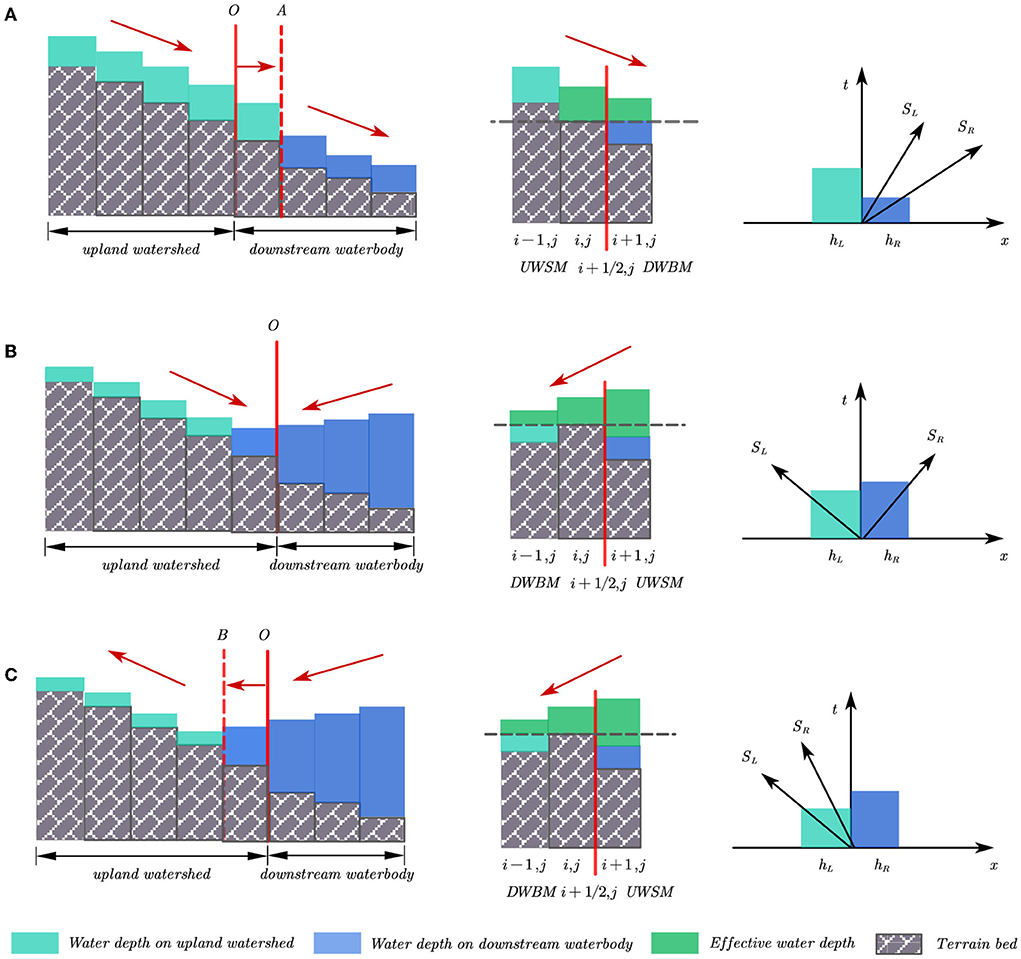
Figure 2. The moving of coupling boundary: (A) from upland watersheds to downstream waterbodies, (B) unchanged, and (C) from downstream waterbodies to upland watersheds.
where is wave velocity (m/s). Since the water depth and flow velocities are variable with time and position, the characteristic wave speeds also change.
If all the wave speeds are positive, that is, SR ≥ SL > 0, the flow velocity of the cell (i, j) is greater than the wave velocity; the discharge of the cell (i, j) flows to the cell (i + 1, j). The coupling interface may move from O to A. The velocity on cell (i, j) is calculated by UWSM. As for the cell (i + 1, j), besides for the change of water depth determined by DWBM, the water volume transferred from cell (i, j) should also be considered. The fluxes calculation on coupling boundary depends on the flow information at cell (i, j), but independent of cell (i + 1, j), which can be calculated as:
Therefore, only the mass conservation through the coupling boundary is transferred and the flow velocity of cells (i, j) and (i + 1, j) cannot affect each other under this situation. The pollutant build-up on the surface is washed by surface runoff, discharged from upland watersheds to downstream waterbodies, which is used as the boundary conditions for the pollutant transport process on the downstream waterbody.
From Figure 2B, if SL < 0 < SR, the coupling interface may remain unchanged at the next time step. The fluxes calculation on coupling boundary depends on the flow information at both cells (i, j) and (i + 1, j). There is interaction between cells (i, j) and (i + 1, j), which means that both the mass and momentum can be transferred through the coupling interface. The fluxes on the coupling interface are calculated:
where
If SL < 0, SR < 0, the coupling interface may move from O to B at the next time step, as the downstream waterbody expands. The fluxes calculation on the coupling boundary only depend on the cell (i + 1, j), as follows:
From Equation (11), both the mass and momentum can be transferred through the coupling interface. And the information related to overland flow and pollutants calculation at cells (i, j) and (i + 1, j) can affect each other.
In the coupling method proposed in this study, surface runoff can flow from upland watersheds to downstream waterbodies, while the impact of floodplain overflow and backwater at confluences are also considered. Consequently, the positions of pollutants discharged into downstream waterbodies change with the moving of inflow boundary. Pollutant distribution in upland watersheds can impact the convection and diffusion of pollutants in downstream waterbodies; conversely, the convection and diffusion of pollutants in downstream waterbodies can also impact that in upland watersheds.
Model validation
In this section, the performance of the E-DBCM was demonstrated by applying it to simulate three cases involving pollutant transport over even and uneven beds. The results were compared with those obtained from VCM, in which the 2D hydrodynamic and water quality calculations featured with identical numerical schemes with DWBM. A stability parameter of 0.5 was used in these cases to enable adaptive time steps.
Pollutant convection in a uniform flow field
The pure convection equation was used to check the reliability of the numerical scheme used in the proposed E-DBCM, which is written as:
The assumed computing regions was an open channel with a flat bottom. The length of the domain was 200 m, and the width was 40 m. The effect of friction resistance was ignored. The initial water depth was 1 m, and the initial velocity was 1 m/s. A rectangular grid, sized Δx = Δy = 1m, was used to discretize the computational zones. It was assumed that there was no rainfall and that the total simulation time was 200 s. The initial pollutant concentrations were as follows:
where L is the range of pollutant distribution (m), and x is the pollutant location.
Additionally, the first-order upwind scheme was used to simulate pollutant convection under the same conditions, and the results were compared with those obtained from E-DBCM, as shown in Figure 3. The simulation results calculated by the E-DBCM were close to the analytical solution, which showed that the numerical format for solving the convection term had desirable accuracy. However, there was significant numerical dissipation of the first-order upwind scheme, so the simulation results obtained from the first-order upwind scheme were significantly lower than the analytical solution. To quantitatively assess the performance of the E-DBCM, the Root Mean Square Error (RMSE) of concentration evolutions was computed. At t = 50s, the RMSEs of E-DBCM and first-order upwind scheme were 0.009 and 0.03, respectively. At t = 100s, those were 0.019 and 0.35, respectively. The RMSE of first-order upwind scheme was larger than that of E-DBCM. It also proved that the proposed model performed well in pollutant transport simulation.
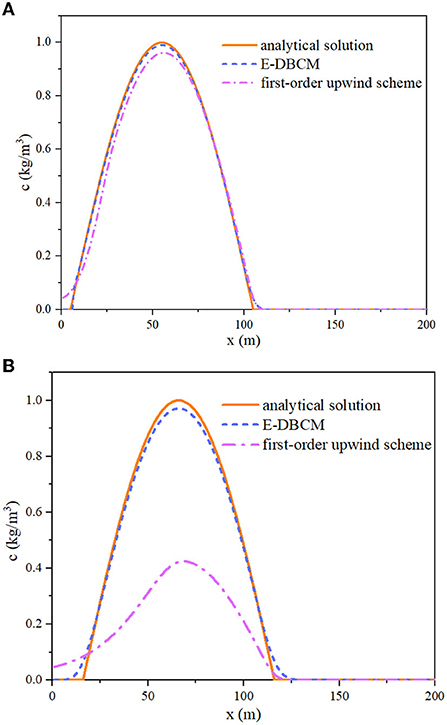
Figure 3. Comparison of the numerical accuracy of different schemes: (A) t = 50s; (B) t = 100s.
Pollutant transport on a slope plane
In this case, pollutant transport over a slope plane (Kim et al., 2012) is developed to evaluate the reliability of the proposed E-DBCM. The length of the plane in this case was 182.88 m and the bed slope was 0.016. As suggested by Kim et al. (2012), the Manning coefficient was 0.025 s/m1/3. The constant rainfall duration was 1,800 s, and the simulations were run for 3,600 s. The initial concentration was determined by Equation (13), and the diffusion coefficients along the x and y directions were all defined as 0.1 m2/s. A rectangular grid was used to discretize the calculation regions, and the grid size was Δx = Δy = 1.83m.
Figure 4 shows the hydrographs at the watershed outlet obtained from different models. The hydrographs obtained from E-DBCM and VCM were consistent with the analytical solution, especially in the discharge rising and receding limbs, indicating that the proposed E-DBCM had reasonable accuracy. However, the hydrographs showed slight differences in the peak discharge. Despite the deviation, the profile of the hydrographs indicated that the proposed E-DBCM had a satisfactory accuracy.
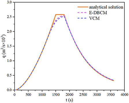
Figure 4. Comparison of hydrographs obtained from different models.
The pollutant concentrations obtained from the E-DBCM and VCM at different times were compared with the analytical solution, as presented in Figure 5. A closer match was produced in the analytical solution and simulation results, indicating encouraging results and a well-captured overall trend. There were small differences between E-DBCM and VCM, especially in the rising limb, which may be caused by the different calculation modules for the surface flow. Overland flow was simulated by the DWBM in the VCM, while the E-DBCM switched from the DWBM to the UWSM when the water depth was lower than the predefined threshold. Therefore, the pollutant concentrations obtained from E-DBCM and VCM varied.

Figure 5. Pollutant concentrations at different times: (A) t = 500s; (B) t = 1, 000s.
The position of the coupling boundary is presented in Figure 6, where the upland watersheds are expressed by green, whereas the downstream waterbodies are marked on yellow. At 1,800 s, the area of downstream waterbodies was higher than that of upland watersheds. The rainfall duration was 1,800 s, and the accumulation rainfall reached a maximum at this time. The water depth in the computational domain was high, which was higher than the predefined threshold in most areas. Therefore, most areas were defined as downstream waterbodies. Once the rainfall ceased, no additional water flowed into the computational domain, and the water depth started to decrease. At 3,600 s, water in the computational domain was shallow, and the water depth was lower than the predefined threshold in most regions. As a result, most areas were considered as upland watersheds. The coupling boundary moved to downstream waterbodies defined at the last moment, and the area of upland watersheds increased. It is clearly observed that the coupling boundary was time-dependent and moved with the changing of water depth, which is in line with the movement process of floods and pollutants.
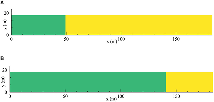
Figure 6. The position of coupling boundary at different times. (A) t = 1,800 s. (B) t = 3,600 s.
Pollutant transport over a plane with varying slope and roughness
In this case, a sloping plan measuring 500m × 400m was designed, with slopes Sox = 0.02 + 0.0000149x and Soy = 0.05 + 0.0000116y along the x and y directions, respectively (Jaber and Mohtar, 2003). The Manning coefficient is equal to , where nx = 0.1 − 0.0000168x and ny = 0.1 − 0.0000168y. The rainfall intensity is given by a symmetric triangular hyetograph r = r(t), with r(0) = r(200min) = 0 and r(100min) = 0.8 × 10⁻⁵m/s. The total simulation time was 14,400 s. The computational domain was divided into several grids with a grid size of Δx = Δy = 10m. The 150m × 150m pollutant cloud was placed in the southwest part of the computational domain; the pollutant concentration was 1 kg/m3. The diffusion coefficients along the x and y directions were 0.2 m2/s. Except for a transmissive boundary at the watershed outlet, the other boundaries were reflective.
The integrated flood modeling system (IFMS) (Wu et al., 2018; Yang et al., 2021) and a model developed by Jaber and Mohtar (2003) were also used to calculate overland runoff. Figure 7 presents the hydrographs obtained from different models. Because very fine grids were used to divide the computational domain to obtain more accurate results in the model developed by Jaber and Mohtar (2003), the results calculated by Jaber and Mohtar (2003) can be considered equivalent to the approximate analytical solution. E-DBCM maintained satisfactory accuracy by holding a shape close to the results simulated by Jaber and Mohtar (2003). However, the peak discharge and receding limb simulated using IFMS were slightly lower than those of the others. Additionally, there were slight differences in the discharge rising limb obtained from E-DBCM and VCM, which may be caused by the different calculation models. The VCM simulated rainfall runoff using the 2D DWBM in the entire domain, whereas the E-DBCM switched from 2D DWBM to UWSM when the water depth was lower than the predefined threshold. When E-DBCM switched from 2D DWBM to UWSM, the method of calculating flow velocities changed, and there was difference in the hydrographs obtained from the VCM and E-DBCM.
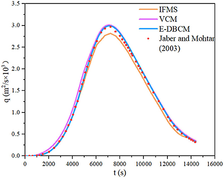
Figure 7. The hydrographs obtained from different models.
The pollutant concentration at the watershed outlet obtained from E-DBCM was compared with that of VCM, as shown in Figure 8. The pollutant concentrations obtained from E-DBCM and VCM were slightly different, which may be caused by the different modules for overland flow. After rainfall, the water depth of the computational domain increased gradually, and the pollutants were transported from upstream to downstream, which took time for pollutants to reach the watershed outlet. Therefore, the pollutant concentration at the downstream outlet was zero at the beginning of rainfall. At ~1,000 s, the pollutants were transported downstream and the pollutant concentration at the watershed outlet began to increase. As observed from this figure, the pollutant concentration first increased and then decreased; the overall change trend of the pollutant concentration was consistent with that of the discharge hydrograph, indicating that dramatically changing floods can cause large-scale water pollution.
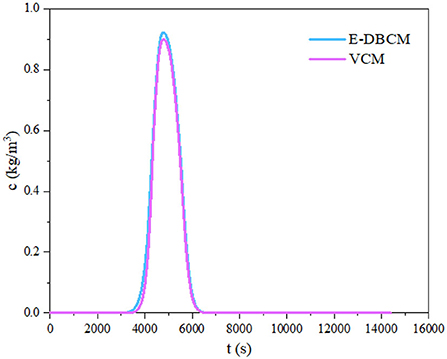
Figure 8. The pollutant concentrations obtained from different models.
The distribution of water depth, position of the coupling boundary, and pollutant concentration contours at different times are shown in Figure 9. At 1,000 s, the water was shallow because of the short rainfall duration and the water depth in most areas was lower than the threshold, as shown in Figure 9a1. Therefore, most of the regions were defined as upland watersheds, and only a small portion of the zones were defined as downstream waterbodies where the DWBM was applied. This is presented in Figure 9a2, where the upland watersheds are marked in green, and the downstream waterbodies are represented in yellow. The pollutants were transported from upstream to downstream with overland flow, but the moving distance was small owing to the short time, as shown in Figure 9a3.
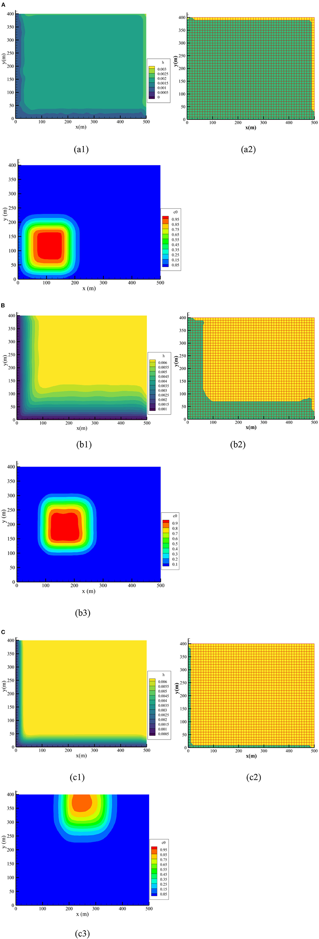
Figure 9. Simulation results at different times. (A) t = 1, 000s: (a1) water depth (m), (a2) position of coupling boundary, and (a3) pollutant concentration (kg/m3). (B) t = 3, 500s (b1) water depth (m), (b2) position of coupling boundary, and (b3) pollutant concentration (kg/m3). (C) t = 6, 000s: (a1) water depth (m), (a2) position of coupling boundary, and (a3) pollutant concentration (kg/m3).
With rainfall development, the accumulated water volume on the surface gradually increased, and the water depth increased over a short period, as presented in Figure 9b1. When the depth was higher than the predefined threshold, the DWBM was applied, and the downstream waterbodies expanded, as presented in Figure 9b2. Accordingly, the coupling interface moved to upland watersheds. The polluted water was discharged downstream with rapid overland flow. Owing to diffusion, the contour of the pollutant concentration changed compared with the initial shape, presented in Figure 9b3.
At 6,000 s, the accumulated rainfall reached its maximum value. The water depth of the basin also reached a maximum, as shown in Figure 9c1. Consequently, the water depth in most regions was higher than the predefined threshold; DWBM was applied in these regions. Therefore, from Figure 9c2, the coupling boundary continued to move to the upland watershed, leading to a large downstream waterbody and a small upland watershed. At this moment, the pollutants were discharged from the computational domain with overland flow, and the pollutant concentration of the computational watershed decreased. The results indicate that the coupling boundary is time-dependent, which is in line with the process of flood and pollutant transport.
Model application
Case study
The Yanqi River Basin is located at Huairou District, Beijing, China, which comprises an area of ~128.7 km2 (Figure 10). Yanqi River Basin is characterized as undulate topography with decreasing from northwest to southeast, and the elevation ranges from 50 to 1,500 m. This basin is in a continental monsoon climate with a mean annual accumulation rainfall of 655 mm. The flood season, a period of frequent rainstorm and flood, spans from June to August every year, during which the rainfall accounts for 60–70% of the total annual rainfall. The tourism industry in this basin is developed, as it has beautiful natural environment. But with the development of tourism, it gives various bad effects on environment. According to statistics, this basin has suffered serious water pollution since the 1990s, and the amount of TP and TN loaded into the river throughout the year are 1,511.52, 9,619.95 kg/a, respectively.
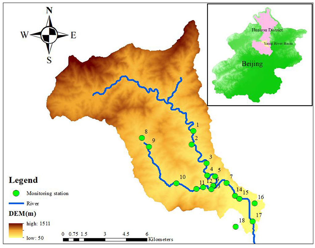
Figure 10. The location of Yanqi River Basin.
The water environmental conditions of Yanqi River Basin were evaluated based on the proposed model. The computational domain was divided into upland watershed and downstream waterbodies, and the spatial size step was Δx = Δy = 50m. The input datasets for E-DBCM include rainfall, DEM, land use, and soil types. Land use was divided into five types: cultivated, forest, grassland, water, and residential areas. Two soil types were identified in the watershed. It was investigated that the TP and TN were the main pollutants in this basin, which were simulated to evaluate the water environment conditions. The initial TP and TN concentrations were 0.5 and 3 mg/L, respectively. Eighteen monitoring stations were installed to monitor the water quality of the basin and their locations are shown in Figure 10. Observed data were used to validate the reliability of the proposed model.
Model calibration and validation
There were so many parameters in the proposed model, such as rainfall intensity, duration, slope, infiltration rate, Manning coefficient, buildup/washoff coefficients, which greatly affect the simulation results. In this section, the Manning coefficient, infiltration coefficient, and buildup/washoff coefficients were calibrated using the observed data at monitoring stations 13 and 14, where more complete and reliable observed data were available, from June 1 to July 20, 2017. The calibrated parameters are listed in Tables B1, B2 in Appendix B. The simulated and observed pollutant concentrations of TP and TN at the different monitoring stations are compared in Figure 11. Percent Bias (PB) and Nash-Sutcliffe efficiency (NSE) were used to assess the model performance (Moriasi et al., 2007). The optimal PB value is 0. The model performed well if the low-magnitude values is <25%. NSE ranges from –∞ to 1.0 (1 inclusive), with NSE = 1 being the optimal value. NSE between 0.0 and 1.0 are generally viewed as acceptable levels of performance.
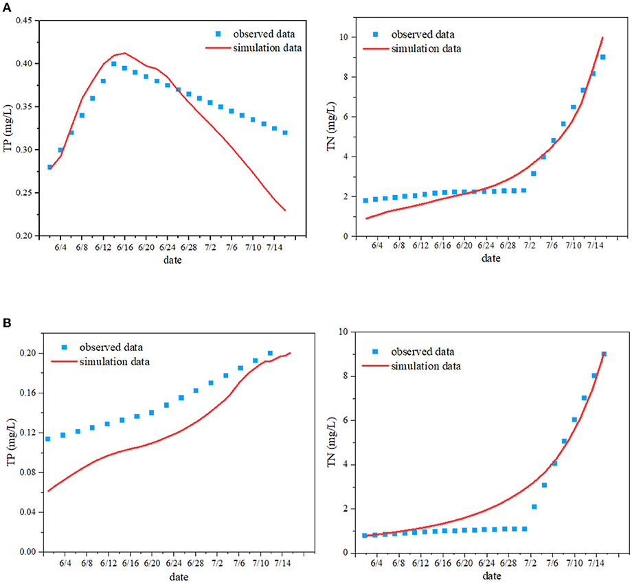
Figure 11. Comparison between observed data and simulation data at monitoring stations 13 and 14. (A) Monitoring station 13. (B) Monitoring station 14.
As presented in Figure 11, the simulation values were correlated with the observed data and the characteristics of the simulated and observed shapes of the pollutant concentrations were very similar, supporting further application of the developed E-DBCM in this basin. However, it is observed that the simulation accuracy of TP and TN is slightly different, which may be caused by the different input parameters, such as washoff/buildup coefficient, washoff exponent. Additionally, there was also uncertainty in the observed data. The NSE and PB of the concentration evolutions at different stations were calculated, as shown in Table 1. The NSE ranged from 0.46 to 0.91. The maximum PB values was 11.3% in these two stations. It is verified again that the proposed E-DBCM performed well for simulating the water environment conditions in this basin.
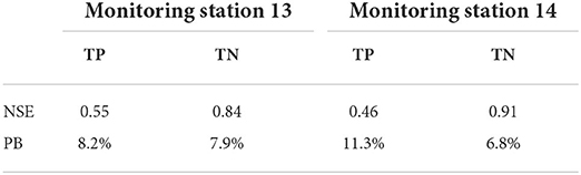
Table 1. The NSE and PB at monitoring stations 13 and 14.
Results and discussions
Figure 12 presents the TP and TN concentrations at the watershed outlet simulated by E-DBCM. The simulated TP concentration showed good agreement with the observed data, especially for the pollutant concentration in the rising and receding limbs. However, the peak concentration was slightly overestimated. During the simulations, the accuracy of the input data, such as infiltration rate, washoff/ buildup coefficient and roughness, can affect the simulation results. Additionally, there was uncertainty in the observed data. The TP concentration increased first and then decreased. In the early stage of simulation, rainfall intensity is relatively large, and pollutants were washed away by rainfall and discharged into the river with the surface flow. As a result, the TP concentration increased rapidly. The TP concentration was >0.4 mg/L, which exceeded the discharge standard of water pollutants in Beijing (DB11/307-2005) and could not satisfy the demand of the water environmental functional district in the Yanqi River Basin. From June to August every year, many tourists visit the Yanqi River Basin, and a lot of catering sewage and domestic wastewater was produced and directly discharged into the river, increasing the pollutant concentration in the river.
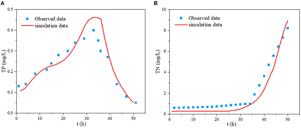
Figure 12. Comparisons of the simulation and observed results: (A) TP; (B) TN.
As shown in Figure 12B, the TN concentration obtained from E-DBCM was consistent with the observed results, indicating that E-DBCM has good performance in practical applications. The TN concentration increased with the development of simulations, which is consistent with the change trend of accumulated rainfall. This concluded that rainfall runoff had a greatly impact on TN concentration. Two reasons can be used to explain this phenomenon. The pollutant accumulated on the surface was washed off by rain and blended with surface runoff, which was the principal causes for the increase of TN concentration. Additionally, sediment pollutants on rivers were continuously released due to the scouring of surface runoff. From the figure, the TN concentration also exceeded the discharge standard of water pollutants in Beijing. Except for the tourism, the flood season in the Yanqi River Basin from June to August is another principal cause for the high pollutant concentration. There were increased rainfall during the flood season, and the erosion effect of rainfall runoff on pollutants was also enhanced. The results show that the proposed model performed well for simulating the pollutant transport in this basin, which can provide basis for the water environment treatment.
The water depth and position of the coupling boundary at different times are presented in Figure 13, where the downstream waterbodies are expressed in yellow whereas the upland watersheds are marked in green. The blue zones represent the non-calculated zones.
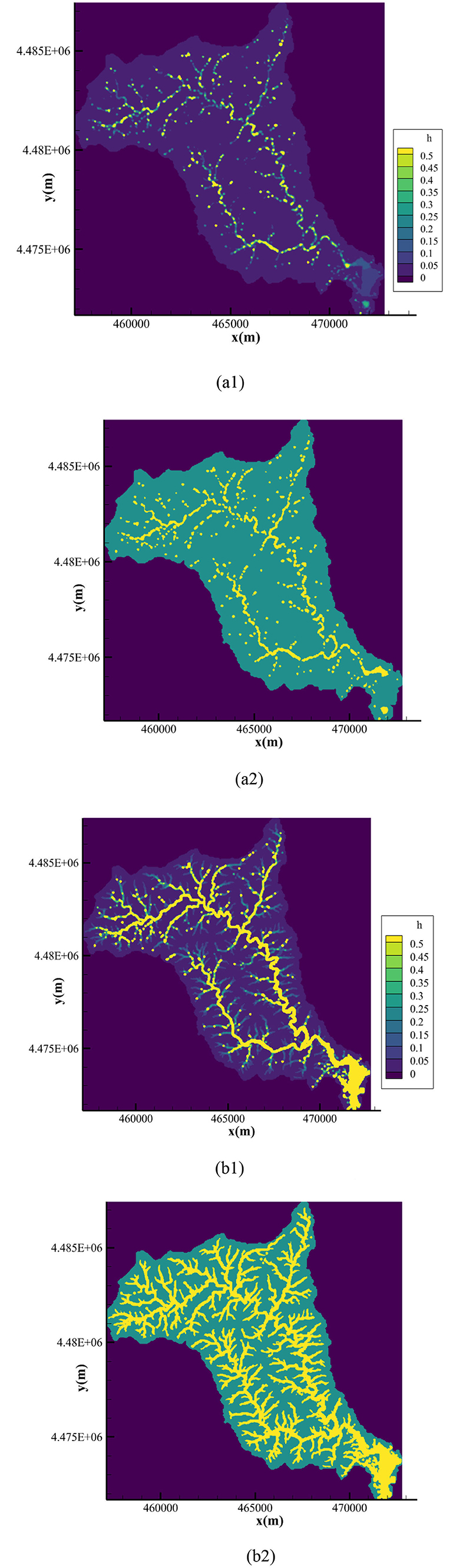
Figure 13. Water depth and the location of coupling interface at different times. (a1) Water depth at t = 2,000 s (m). (a2) Upland watershed and downstream waterbody at t = 2,000 s. (b1) Water depth at t = 70,000 s (m). (b2) Upland watershed and downstream waterbody at t = 70,000 s.
It is observed from this figure that the coupling boundary was time-dependent and moved with the changing of water depth. At t = 2, 000s, the accumulation rainfall is small at the starting of the rainfall. From Figure 13a1, except for the main channel, the water depth in most regions was small, which is lower than the predefined threshold. Therefore, as Figure 13a2 shows, small area in the basin were defined as downstream waterbodies, while the rest were determined as upland watersheds. At 19 h, water depth in this basin raised with the development of rainfall, as shown in Figure 13b1. The water depth in most areas was higher than the predefined threshold at this moment. Consequently, the coupling boundary moved to the upland watershed defined at the last moment, as the downstream waterbodies expanded, as presented in Figure 13b2.
Conclusions
A dynamic bidirectional coupled framework of the UWSM and 2D DWBM for watershed water quality simulation was proposed in this study. The computational regions were divided into upland watersheds and downstream waterbodies. A water depth threshold was proposed to determine the upland watersheds and downstream waterbodies. If the water depth was above the threshold, it was determined as downstream waterbodies, where the 2D DWBM was used to simulate the convention and diffusion process of pollutants; conversely, if the water depth was lower than the predefined threshold, it could be considered as upland watersheds, where the pollutants load and transport were calculated by the UWSM. The UWSM and DWBM were coupled by a moving interface, which can realize the time synchronization of the UWSM and 2D DWBM and ensure the mass and momentum conservation through the coupling interface.
Three cases were designed to evaluate the reliability of the proposed E-DBCM. The simulation results obtained from the E-DBCM were close to the analytical solution in both flow and pollutant concentration profiles, which indicated that the E-DBCM performed well for simulating the pollutant transport and flood processes. A moving coupling boundary was also observed in these cases. The water environment conditions in the Yanqi River Basin were assessed based on the proposed E-DBCM. The simulation results were consistent with the observed data, indicating that the E-DBCM had good performance on practical applications. The TP concentration in the Yanqi River Basin increased first and then decreased, while the TN concentration continually increased. The tourism and the flood season were the two main reasons causing water quality pollution in this basin. It is essential to take measures to protect the water environment and improve water environment treatment capacity.
Presently, the proposed E-DBCM is more suitable for small and medium watersheds on an event time scale, but it may require more computation time while improving the calculation accuracy, which needs to be further improved. Notably, the area of the upland watershed is much greater than that of waterbodies. The fine grids are required to be applied to waterbodies, that is the middle and lower reaches of rives, which are vulnerable to pollution. But upstream these areas, usually there is no need to apply the fine grids, and coarse grids are acceptable and indeed recommended. In the future, the application of multigrid technology in upland watersheds and downstream waterbodies can reduce computing time. In addition, the chemical reaction of pollutants in waterbodies is also important, it is necessary to study the pollutant degradation in waterbodies in the future, such as developing the coupling of E-DBCM and eco-toxicology models.
Data availability statement
The raw data supporting the conclusions of this article will be made available by the authors, without undue reservation.
Author contributions
Material preparation, data collection, and analysis were performed by CJ and ZZ. The first draft of the manuscript was written by YS. YS, ZZ, and CJ commented on previous versions of the manuscript. All authors contributed to the study conception, design, read, and approved the final manuscript.
Funding
This study was supported by the National Science Foundation of China (No. 52179068) and Key Laboratory of Hydroscience and Engineering (No. 2021-KY-04).
Acknowledgments
The authors thank reviewers for their valuable comments.
Conflict of interest
The authors declare that the research was conducted in the absence of any commercial or financial relationships that could be construed as a potential conflict of interest.
Publisher's note
All claims expressed in this article are solely those of the authors and do not necessarily represent those of their affiliated organizations, or those of the publisher, the editors and the reviewers. Any product that may be evaluated in this article, or claim that may be made by its manufacturer, is not guaranteed or endorsed by the publisher.
Supplementary material
The Supplementary Material for this article can be found online at: https://www.frontiersin.org/articles/10.3389/frwa.2022.986528/full#supplementary-material
References
Arnold, J. G., Moriasi, D. N., Gassman, P. W., Abbaspour, K. C., White, M. J., Srinivasan, R., et al. (2012). SWAT: model use, calibration, and validation. Transact. ASABE 55, 1491–1508. doi: 10.13031/2013.42256
Bicknell, B. R., Imhoff, J. C., Kittle, J. L., Jobes, T. H., Donigian, A. S. Jr., and Johanson, R. (2001). Hydrological Simulation Program–Fortran: HSPF, Version 12 User's Manual. Mountain View, CA: AQUA TERRA Consultants, 845.
Bradbrook, K. F., Lane, S. N., Waller, S. G., and Bates, P. D. (2004). Two-dimensional diffusion wave modelling of flood inundation using a simplified channel representation. Int. J. River Basin Manag. 3, 211–223. doi: 10.1080/15715124.2004.9635233
Brown, L. C., and Barnwell, T. O. (1987). The enhanced stream water quality models QUAL2E and QUAL2EUNCAS: Documentation and user manual. Athens: US Environmental Protection Agency. Office of Research and Development. Environmental Research Laboratory, 189.
Danish Hydraulic Institute (2009). The MIKE SHE User and Technical Reference Manual. Copenhagen: Danish Hydraulic Institute.
Delis, A., and Nikolos, I. (2013). A novel multidimensional solution reconstruction and edge-based limiting procedure for unstructured cell-centered finite volumes with application to shallow water dynamics. Int. J. Numer. Methods Fluids 71, 584–633. doi: 10.1002/fld.3674
Fu, B., Horsburgh, J. S., Jakeman, A. J., Gualtieri, C., Arnold, T., Marshall, L., et al. (2020). Modeling water quality in watersheds: From here to the next generation. Water Resour. Res. 56, e2020WR027721. doi: 10.1029/2020WR027721
Gülbaz, S. (2019). Water quality model for nonpoint source pollutants incorporating bioretention with EPA SWMM. Desal. Water Treat. 164, 111–120. doi: 10.5004/dwt.2019.24684
Hou, J. M., Shi, B. S., Liang, Q. H., Tong, Y., Kang, Y. D., Zhang, Z. A., et al. (2021). A graphics processing unit-based robust numerical model for solute transport driven by torrential flow condition. J. Zhejiang Univ. Sci. A 22, 835–850. doi: 10.1631/jzus.A2000585
Hwang, S., Jun, S. M., Song, J. H., Kim, K., Kim, H., and Kang, M. S. (2021). Application of the SWAT-EFDC linkage model for assessing water quality management in an estuarine reservoir separated by levees. Appl. Sci. 11, 3911–3911. doi: 10.3390/app11093911
Jaber, F. H., and Mohtar, R. H. (2003). Stability and accuracy of two-dimensional kinematic wave overland flow modeling. Adv. Water Resour. 26, 1189–1198. doi: 10.1016/S0309-1708(03)00102-7
Kashyap, S., Dibike, Y., Shakibaeinia, A., Prowse, T., and Droppo, I. (2017). Two-dimensional numerical modelling of sediment and chemical constituent transport within the lower reaches of the Athabasca River. Environ. Sci. Pollut. Res. 24, 2286–2303. doi: 10.1007/s11356-016-7931-3
Kim, J., Warnock, A., Ivanov, V. Y., and Katopodes, N. D. (2012). Coupled modeling of hydrologic and hydrodynamic processes including overland and channel flow. Adv. Water Resour. 37, 104–126. doi: 10.1016/j.advwatres.2011.11.009
Kong, J., Xin, P., Shen, C. J., Song, Z. Y., and Li, L. (2013). A high-resolution method for the depth-integrated solute transport equation based on an unstructured mesh. Environ. Modell. Softw. 40, 109–127. doi: 10.1016/j.envsoft.2012.08.009
Li, B., Yang, G., Wan, R., and Li, H. (2018). Hydrodynamic and water quality modeling of a large floodplain lake (Poyang Lake) in China. Environ. Sci. Pollution. Res. 25, 35084–35098. doi: 10.1007/s11356-018-3387-y
Moriasi, D. N., Arnold, J. G., Van Liew, M. W., Bingner, R. L., Harmel, R. D., and Veith, T. L. (2007). Model evaluation guidelines for systematic quantification of accuracy in watershed simulations. Transact. ASABE 50, 885–900. doi: 10.13031/2013.23153
Narasimhan, B., Srinivasan, R., Bednarz, S. T., Ernst, M. R., and Allen, P. M. (2010). A comprehensive modeling approach for reservoir water quality assessment and management due to point and nonpoint source pollution. Transact. ASABE 53, 1605–1617. doi: 10.13031/2013.34908
Shi, Q., Zhan, J., Wu, F., Deng, X., and Xu, L. (2012). Simulation on water flow and water quality in Wuliangsuhai lake using a 2-D hydrodynamic model. J. Food Agric. Environ. 10, 973–975. Available online at: https://www.ccap.pku.edu.cn/docs/20171229202007087876.pdf
Shin, S., Her, Y., Song, J. H., and Kang, M. S. (2019). Integrated sediment transport process modeling by coupling soil and water assessment tool and environmental fluid dynamics code. Environ. Modell. Softw. 116, 26–39. doi: 10.1016/j.envsoft.2019.02.002
Toro, E. F. (2001). Shock-Capturing Methods for Free-Surface Shallow Flows. New York, NY: John Wiley.
Toro, E. F., Spruce, M., and Speares, W. (1994). Restoration of the contact surface in the HLL-Riemann Solver. Shock Waves 4, 25–34. doi: 10.1007/BF01414629
Van Leer, B. (1979). Towards the ultimate conservative difference scheme V: a second order sequel to Godunov's method. J. Comput. Phys. 32, 101–136. doi: 10.1016/0021-9991(79)90145-1
Wang, P., Wang, C. H., Hua, Z. L., Wei, Y. P., Ma, T. F., Shen, X., et al. (2020). A structurally integrated water environmental modeling system based on dual object structure. Environ. Sci. Pollut. Res. 27, 11079–11092. doi: 10.1007/s11356-020-07669-9
Wang, Z., Fu, R., Wang, D., Zhang, X., and Lai, X. (2021). “Coupling simulation of non-point source pollution and 2-D water quality in Nanhe river,” in IOP Conference Series: Earth and Environmental Science (Chengdu), 8.
Wool, T. A., Ambrose, R. B., Martin, J. L., and Comer, E. A. (2006). Water Quality Analysis Simulation Program (WASP), Version 6.0, User's Manual. Atlanta, GA: US EPA, 267.
Wu, J., Yan, R., and Song, J. (2018). Effectiveness of low-impact development for urban inundation risk mitigation under different scenarios: a case study in Shenzhen, China. Nat. Hazards Earth Syst. Sci. 18, 2525–2536. doi: 10.5194/nhess-18-2525-2018
Xue, B., Zhang, H., Wang, Y., Tan, Z., and Shrestha, S. (2021). Modeling water quantity and quality for a typical agricultural plain basin of northern China by a coupled model. Sci. Total Environ. 790, 148139. doi: 10.1016/j.scitotenv.2021.148139
Yang, B., Ma, J., Huang, G., and Cao, D. (2021). “Development and application of 3D visualization platform for flood evolution in Le'an river basin of Wuyuan,” in IOP Conference Series Earth and Environmental Science (Dali), 9.
Yang, X., Tan, L., He, R., Fu, G., and Wang, G. (2017). Stochastic sensitivity analysis of nitrogen pollution to climate change in a river basin with complex pollution sources. Environ. Sci. Pollut. Res. 24, 26545–26561. doi: 10.1007/s11356-017-0257-y
Yu, C., and Duan, J. G. (2017). Simulation of surface runoff using hydrodynamic model. J. Hydrol. Eng. 22, 04017006. doi: 10.1061/(ASCE)HE.1943-5584.0001497
Yuan, L., Sinshaw, T., and Forshay, K. J. (2020). Review of watershed-scale water quality and nonpoint source pollution models. Geosciences 10, 25. doi: 10.3390/geosciences10010025
Appendix A: pollutant load module
In UWSM, SNPS,k is solved by a pollutant load module consisting of build-up and wash-off processes, as follows:
1. Pollutant build-up process
Pollutants accumulate on the land surface during periods of dry weather and can be discharged into rivers via runoff during rain events. The accumulated pollutants are calculated using an exponential function (Gülbaz, 2019). It is considered that the pollutant accumulation follows an exponential curve that asymptotically approaches the maximum limit. The calculation equation is as follows:
where Bk is the accumulation of k-th pollutant per unit area (kg/ha); C1 is the maximum build-up on the sub-basin surface (kg/ha); C2 is the build-up rate constant (day−1); t is the build-up time.
2. Pollutant wash-off process
During rainy days, the pollutants accumulate on the surface and are then washed off by rain and blend with the surface runoff. The wash-off of pollutants is calculated using the wash-off function. The wash-off function is given by Equation (A2), which can simulate the variation in pollutant load with spatial location and time.
where SNPS is the wash-off of pollutants per unit area [kg/(m2·s)]; is the wash-off coefficient [(mm/h)−C4·h−1]; C4 is the wash-off exponent (dimensionless), and q is the runoff rate per unit area (mm/h).
Appendix B: Calibrated parameters of proposed E-DBCM in Yanqi River Basin

Table B1. Parameters related to pollutant load calculation of different land use.
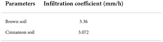
Table B2. Infiltration coefficient of different soils.
Keywords: watershed water environment, UWSM, 2D DWBM, E-DBCM, dynamic bidirectional coupling model
Citation: Shen Y, Zhu Z and Jiang C (2022) E-DBCM: A dynamically coupled upland and in-stream water quality model for watershed water quality simulation. Front. Water 4:986528. doi: 10.3389/frwa.2022.986528
Received: 05 July 2022; Accepted: 01 September 2022;
Published: 20 September 2022.
Edited by:
Qian Zhang, University of Maryland, United StatesReviewed by:
Wei Zhi, The Pennsylvania State University (PSU), United StatesCaihong Hu, Zhengzhou University, China
Copyright © 2022 Shen, Zhu and Jiang. This is an open-access article distributed under the terms of the Creative Commons Attribution License (CC BY). The use, distribution or reproduction in other forums is permitted, provided the original author(s) and the copyright owner(s) are credited and that the original publication in this journal is cited, in accordance with accepted academic practice. No use, distribution or reproduction is permitted which does not comply with these terms.
*Correspondence: Chunbo Jiang, jcb@tsinghua.edu.cn