 Jing Deng1,2*
 Anaïs Couasnon1
 Ruben Dahm1
 Markus Hrachowitz2Klaas-Jan van Heeringen1Hans Korving1
 Albrecht Weerts1,3
 Riccardo Taormina2
- 1Deltares, Delft, Netherlands
- 2Department of Water Management, Faculty of Civil Engineering and Geosciences, Delft University of Technology, Delft, Netherlands
- 3Hydrology and Environmental Hydraulics Group, Department of Environmental Sciences, Wageningen University and Research, Wageningen, Netherlands
This study focuses on exploring the potential of using Long Short-Term Memory networks (LSTMs) for low-flow forecasting for the Rhine River at Lobith on a daily scale with lead times up to 46 days ahead. A novel LSTM-based model architecture is designed to leverage both historical observation and forecasted meteorological data to carry out multi-step discharge time series forecasting. The feature and target selection for this deep learning (DL) model involves evaluating the use of different spatial resolutions for meteorological forcing (basin-averaged or subbasin-averaged), the impact of incorporating past discharge observations, and the use of different target variables (discharge Q or time-differenced discharge dQ). Then, the model is trained using the ERA5 dataset as meteorological forcing, and employed for operational forecast with ECMWF seasonal forecast (SEAS5) data. The forecast results are compared to a benchmark process-based model, wflow_sbm. This study also explores the flexibility of the DL model by fine-tuning the pretrained model with limited SEAS5 dataset. Key findings from feature and target selection include: (1) opting for subbasin-averaged meteorological variables significantly improves model performance compared to a basin-averaged approach. (2) Utilizing dQ as the target variable greatly boosts short-term forecast accuracy compared to using Q, with a mean absolute error (MAE) of 25 m3 s−1 and mean absolute percentage error (MAPE) of 0.02 for the first lead time, ensuring reliability and accuracy at the onset of the forecast horizon. (3) While incorporating historical discharge improves the forecasting of Q, its impact on predicting dQ is less pronounced for short lead times. In the operational forecast with SEAS5, compared to the wflow_sbm model, the DL model exhibits skill in forecasting low flows as evidenced by Continuous Ranked Probability Skill Score (CRPSS) median values of all lead times above zero, and better accuracy in forecasting drought events within short lead times. The wflow_sbm model shows higher accuracy for longer lead times. In the exploration of fine-tuning approach, the fine-tuned model generates marginal short-term enhancements in forecasting low-flow events over a non-fine-tuned model. Overall, this study contributes to advancing the field of low-flow forecasting using deep learning approach.
1 Introduction
Since the beginning of the twenty-first century, Europe has experienced a series of severe droughts (2003, 2015, 2018, and 2022), affecting a wide range of socio-economic sectors including agriculture, energy production, waterborne transportation, public water supply and freshwater ecosystem (EEA, 2010; Ionita et al., 2017; WMO, 2020). Under future warmer climate, drought events are projected to occur more frequently with increasing impacts in many regions and river basins (Prudhomme et al., 2014; Wanders and Van Lanen, 2015; van der Wiel et al., 2019; Cammalleri et al., 2020). Given the potential widespread impacts of droughts, better understanding and preparing for this hazard is important.
Droughts are generally classified into four categories, closely linked to water (shortage) moving through the water cycle and its use (Wilhite and Glantz, 1985; Tallaksen and Van Lanen, 2004; Van Loon, 2015): meteorological drought, soil moisture drought, hydrological drought, and socioeconomic drought. It has both natural and human drivers (Van Loon et al., 2016). Streamflow drought or low flow, which is a part of hydrological drought, is here defined as below-normal river discharge. It is a result of climate variability, catchment characteristics and anthropogenic influences (Van Loon and Van Lanen, 2012; Van Lanen et al., 2013; Van Loon, 2015). The Netherlands has experienced severe drought events during the summer in recent years. The 2018 drought event, especially, was marked by a country-average annual precipitation of 607 mm, 240 mm less than normal, and prolonged low river discharges which had significant impact on shipping and external salinization (Kramer et al., 2019).
The Netherlands heavily relies on a large transboundary river, i.e., the Rhine, for freshwater supply. The Rhine enters the Netherlands at Lobith, making it a key location for water management decisions in the country. Knowing how much water enters the Netherlands at Lobith and how much to expect over subsequent days and weeks determines the navigable depth for shipping and the water distribution, especially for the Klimaatbestendige Wateraanvoer (KWA, Climate-Resilient Water Supply system), in a large part of the country. When the discharge at Lobith drops below specific thresholds, operational measures need to be taken to distribute river water according to the priority water use sequence defined by the national water authorities (Rijkswaterstaat, 2019). Therefore, a reliable and robust forecasting of low flows at Lobith is essential for Dutch water managers and stakeholders to develop robust strategies for drought mitigation and adaptation. Different drought impact sectors require different forecasting lead times. Two-week forecasts are generally required by the freight shipment sector, while longer lead time forecasts of several weeks or months are crucial references for water distribution strategies (Demirel et al., 2013; Van Loon, 2015).
Forecasting low flows for the Rhine River for longer lead times has been subject of several studies (Demirel et al., 2013; e.g., Yossef et al., 2013; Klein and Meißner, 2018; Hurkmans et al., 2023). Most of these studies report some skill for predicting low flows with lead times of up to 6–8 weeks for the spring and early summer periods when low flows are driven by snowpack and/or wetness of soil and groundwater system. However, the forecast skill tends to diminish for other times of the year with lead times ranging from 2–4 weeks. All the mentioned studies make use of conceptual hydrological or land surface models, except for Demirel et al. (2013) who used a simple regression analysis.
Over the past few years, data-driven approaches, such as deep learning (DL) models, have been explored and tested for applications in hydrology (Shen, 2018; Shen et al., 2021). In particular, studies have shown that Long Short-Term Memory (LSTM) models have the potential to be effective tools for the dynamic modeling of streamflow (Kratzert et al., 2019b) and soil moisture (Fang et al., 2017), which has led to an increase in the use of DL techniques across all domains of hydrology. Most studies on drought forecasting using DL focus on predicting drought indices such as meteorological drought indices Standardized Precipitation Index (SPI) and Standardized Precipitation and Evapotranspiration Index (SPEI) (Dikshit et al., 2022), as well as hydrological drought indices Streamflow Drought Index (SDI) (Borji et al., 2016; Shamshirband et al., 2020; Aghelpour et al., 2021) on a monthly scale. On the other hand, there are relatively few studies using DL techniques to forecast low-flow time series on a daily scale. Sahoo et al. (2019) developed LSTMs and other recurrent neural network models to predict one-step-ahead monthly low-flow time series using the past 2 months' low-flow values. Amanambu et al. (2022) used a transformer and a LSTM model with past daily stage level as input to predict stage levels multiple steps ahead (i.e., 30, 60, 90, 120, and 180 days), which were then post-processed to generate the numbers of drought days using the threshold approach. However, these studies feature only strictly autoregressive models without incorporating predictors such as the meteorological forcing. More importantly, very few studies consider the deployment of trained DL models in an operational framework where forecasted meteorological forcing data can provide additional information for long-term, multi-step ahead time series forecasting. Hauswirth et al. (2023) employed five different machine learning models, including LSTMs, trained on historical observations of discharge, precipitation, evaporation, and seawater levels. These models were then run with seasonal (re)forecast data of these driver variables in a hindcast setting to predict hydrological variables and were assessed on the capability to simulate low-flow events using the threshold approach. Franken et al. (2022) used a LSTM-based encoder-decoder approach to integrate historical and forecasted meteorological data as well as discharge observations for low-flow forecasts in Flanders on short (72 h) and long (30 days) time horizons. Similar encoder-decoder approaches have also been used by several other research on operational streamflow forecasting, such as Google's operational flood forecasting system (Nevo et al., 2022) and the study by Kao et al. (2020) on multi-step-ahead flood forecasting.
This study aims to investigate the potential of LSTMs for low-flow forecasting for the Rhine River at Lobith on a daily scale, with lead times up to 46 days ahead which is in line with the current forecasting system used by the national water authorities with European Center for Medium-Range Weather Forecasts (ECMWF) extended range forecasts. To do this, we design a model architecture that can leverage both historical observations and forecasted meteorological data to predict the discharge at Lobith multiple days ahead. The search for the optimal model architecture involves an evaluation of multiple factors, including different spatial resolutions of meteorological forcing, the impact of incorporating past discharge observations, and the use of different target variables. Then, the model setup is used for operational forecast with ECMWF seasonal forecast (SEAS5) data. The forecast results are compared to a benchmark process-based model, the wflow_sbm model, a state-of-the-art distributed hydrological model set up for the Rhine (Imhoff et al., 2020). This study also explores the flexibility of the DL approach by fine-tuning the pretrained model with limited SEAS5 dataset, aiming to make the most of the available data. The forecast results from the fine-tuned model are compared with the ones without fine-tuning.
The paper is structured in the following way: Section 2 describes the study area, the data, and the model architecture tested. Next, three experiment designs are described: the first experiment explores the effect of selecting different feature and target variables on the DL model performance. The second experiment investigates the capability of the DL model for operational forecast with the SEAS5 data. The third experiment tests whether the SEAS5 fine-tuned model can help to enhance the forecast performance. Section 3 presents the results and discussions of the experiments. Section 4 shows the limitations of this study and proposes future works. The paper concludes with a summary in Section 5.
2 Materials and methods
2.1 Study area
The Rhine originates in Switzerland, flowing along a 1,230 km course before draining into the North Sea. The Rhine basin has an area of around 185,000 km2, covering major parts of Switzerland and Luxembourg, and parts of Germany, France, Italy, Austria, and the Netherlands. The elevation of the basin varies from around 4,000 m above sea level in the Alps to sea level in the Netherlands.
The Rhine River basin upstream of Lobith can be divided into eight subbasins shown in Figure 1, displaying different discharge behaviors. The southern alpine area is a snow-driven regime, characterized by the interplay of winter snow cover, summer snowmelt, and relatively high summer precipitation. As a result, low flows in this region occur mainly in winter and flood events mainly in summer. Subbasins such as the Neckar, Main, and Moselle, which drain the lower, pre-alpine hill regions, exhibit a rain-driven regime. This regime is characterized by a dominance of winter floods and summer low flows. In downstream areas of the Middle and Lower Rhine, including Lobith, where the snow regime and rain regime overlap, a combined regime is observed. The discharge is more evenly distributed throughout the year (International Commission for the Protection of the Rhine, 2018).
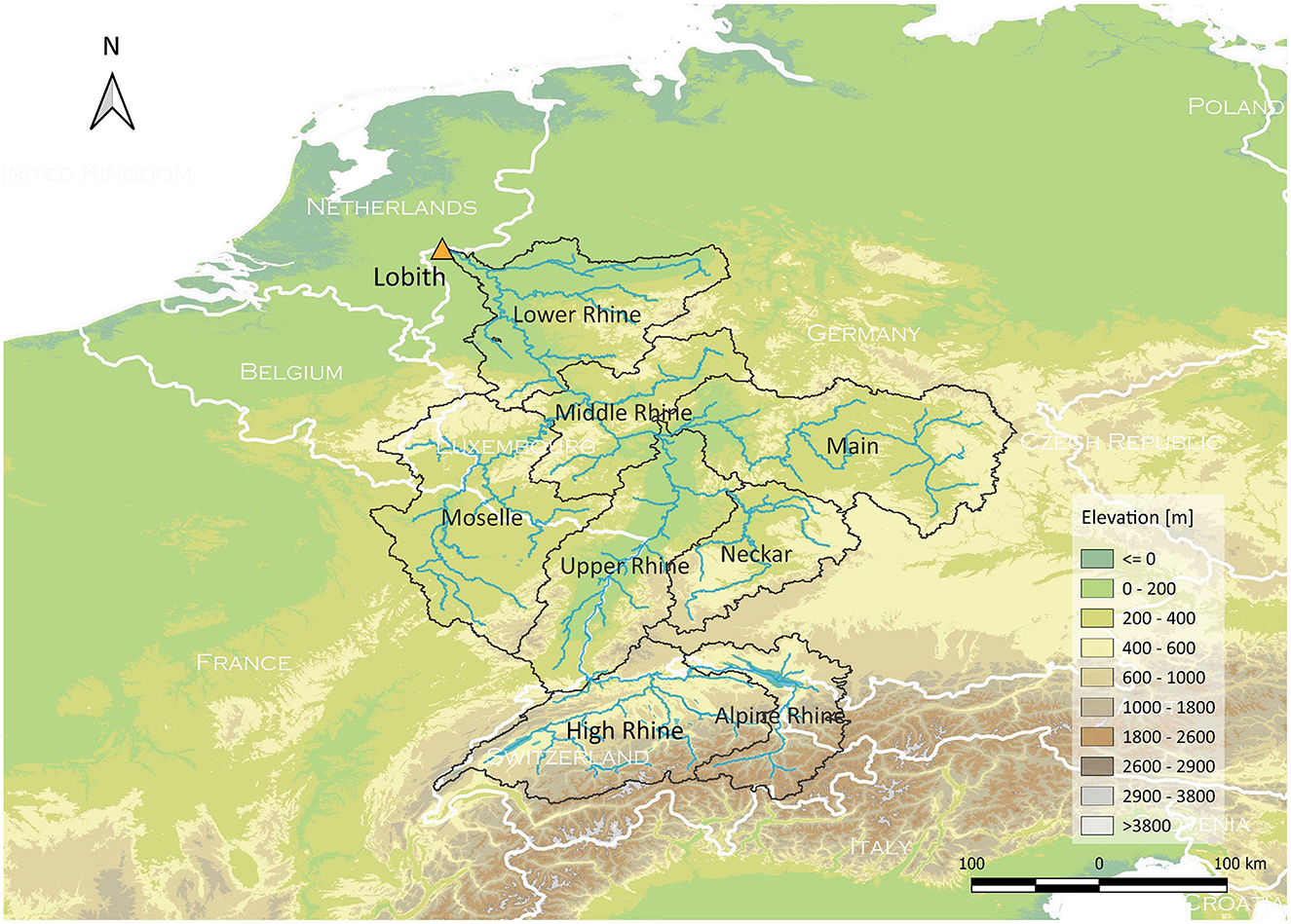
Figure 1. Eight subbasins of the Rhine River basin upstream of Lobith.
The river discharge climatology at Lobith based on different 10-year periods is shown in Figure 2. The average discharge at Lobith is highest in winter months (around December to March), most of which originates from tributaries in the subbasins Neckar, Main and Moselle characterized by intense rainfall and low evaporation. Only 30% of the discharge at Lobith during winter months is from the Alps, as winter precipitation falls as snow (Middelkoop and van Haselen, 1999). During the summer months (around July to September), more than 70% of the discharge at Lobith originates from the Alps (Middelkoop and van Haselen, 1999). Less is from other parts of the basin, as much of summer precipitation in other subbasins evaporates before it reaches the river.
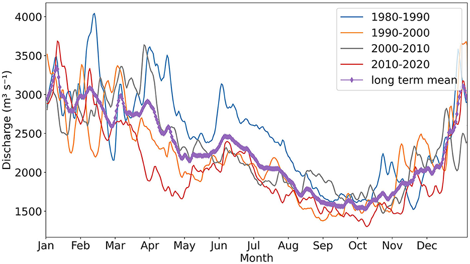
Figure 2. River discharge climatology at Lobith based on different 10-year periods (Data source: Rijkswaterstaat Waterinfo; see footnote1).
2.2 Data
In this study, we design a deep learning model to forecast daily discharge at Lobith with lead times up to 46 days ahead. Three meteorological variables – daily total precipitation (tp), daily average 2-meter temperature (t2m), and daily total potential evaporation (pev) – are used as predictors to describe the meteorological conditions over time. We also explore the incorporation of past daily average discharge observations at Lobith as additional predictor. An overview of the data used in this research is presented hereafter, while detailed data processing steps are provided in the Supplementary material.
2.2.1 Discharge at Lobith
The daily average discharge observations at Lobith for the period 1979–2022 were obtained from the Rijkswaterstaat Waterinfo website1. During dry periods, when the discharge at Lobith is lower than a certain threshold (Table 1), operational measures need to be taken to distribute the available water among all water users. Therefore, in this study, we define low-flow events at Lobith as instances when the discharge falls below the river discharge threshold outlined in Table 1.
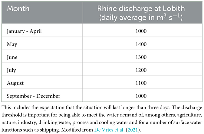
Table 1. River discharge threshold at Lobith for scaling up from level 0 (normal management) to level 1 (impending water shortages).
2.2.2 Meteorological data
For the observation data of daily meteorological variables for the period 1979–2022, we used two different products, the E-OBS and ERA5 datasets. Section 2.4 further details how they were used in each experiment. The E-OBS dataset (Cornes et al., 2018) provides spatially interpolated estimates derived from in-situ observations at meteorological stations across Europe which are provided by the National Meteorological and Hydrological Services (NMHSs) and other data holding institutes, with spatial resolutions of 0.1 degree. The ERA5 dataset (Hersbach et al., 2023) is the fifth-generation climate reanalysis of ECMWF providing atmospheric variables with global coverage at a spatial resolution of 0.25 degree. Recent research suggests that ERA5 can be an effective input for rainfall-runoff modeling using LSTMs, despite its coarser resolution compared to local forcing datasets (Wilbrand et al., 2023).
For the forecast data of meteorological variables, we use the SEAS5 dataset (Johnson, 2019). The SEAS5 is the fifth generation of the ECMWF seasonal forecasting system. It is initialized every first day of each month, and provides forecasts up to 7 months ahead for 51 ensemble members on a daily scale. The SEAS5 dataset used in this study has a spatial resolution of 0.25 degree and has been bias corrected using scaled distribution mapping (Switanek et al., 2017) with ERA5 dataset as observational dataset which is also used to initialize the wflow_sbm model. Since SEAS5 does not provide potential evaporation information directly, the Makkink method (De Bruin, 1987) is applied to compute gridded potential evaporation using the 2-m temperature and incoming shortwave radiation, both of which are directly available from the dataset. Note that there can be a difference between the Makkink method used here and the method employed in ERA5 for generating potential evaporation. However, previous research (van Osnabrugge et al., 2019) found that the impact of potential evaporation forcing type on the Rhine River streamflow forecast is limited.
2.3 Model architecture
In the field of streamflow modeling, more recent studies have found DL techniques, such as LSTM, to be a promising approach, providing improvements in prediction accuracy, scalability, and regional generalization compared to conventional conceptual models (e.g., Mosavi et al., 2018). LSTM models, specifically designed for processing sequential data like time series, have been successfully applied by Kratzert et al. (2018, 2019a) in over 500 basins across the United States, demonstrating that LSTMs trained on large-sample hydrological datasets are effective tools for rainfall-runoff modeling. Since then, these recurrent neural networks have been widely adopted as the preferred data-driven methods for streamflow prediction and forecasting (Frame et al., 2022; Hunt et al., 2022; Nearing et al., 2023; Wilbrand et al., 2023). Therefore, in this study, the decision is made to build a DL model based on the LSTM architecture. A detailed description of LSTM architecture can be found in Kratzert et al. (2018).
We design a novel model architecture based on LSTMs, addressing the need to (1) effectively leverage both historical observation and forecast data within a single DL model, and (2) carry out multi-step time series forecasting. An illustration of the model structure is shown in Figure 3. The architecture utilizes two LSTM models, with one LSTM (LSTM-1) processing historical observation data and another LSTM (LSTM-2) processing forecast data. The outputs of LSTM-2 are then fed into the Dense layer, which produces the final output of 46 predictions simultaneously.
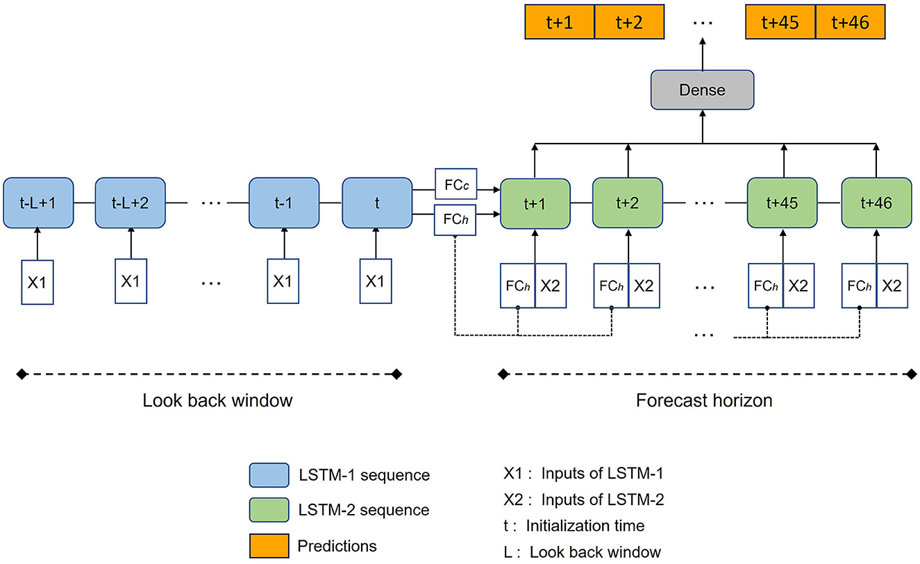
Figure 3. Schematic illustration of the model architecture used in this study.
This model structure is inspired by the historical and forecast modes of operation in process-based operational streamflow forecast model (Weerts, 2009). LSTM-1 processes sequential observation data from past L days (X1). The processing continues up until the forecast initialization time (t). The final cell state and hidden state of LSTM-1 are passed through a fully connected layer FCc and FCh respectively, and the resulting states are used as the initial cell state and hidden state for LSTM-2. The use of fully connected layers to transfer states between the two LSTMs is inspired by Gauch et al. (2021) where the transferred states allow the generation of predictions at multiple timescales. The resulting hidden state is also concatenated with the input of LSTM-2 (X2) at each time step, aiming to help LSTM-2 retain and utilize the historical information summarized by LSTM-1. This choice is inspired by the work of Wang et al. (2019), where a sequence-to-sequence model is used with a vectorized history representation of dialog history to enhance response generation for generative conversational agents. Along with this additional context, LSTM-2 processes forecast data and returns the full sequence of outputs to the Dense layer. The Dense layer subsequently changes the output's dimensionality from the preceding layer to 46 predictions.
The model uses a historical sequence length of 270 days (Kratzert et al., 2019b) for X1, and a forecast sequence length of 46 days for X2. A less extensive hyperparameter tuning is conducted for this model architecture, as the hyperparameters of the LSTM model for streamflow prediction have been studied and optimized by several studies (Kratzert et al., 2018, 2019b; Gauch et al., 2021; Nevo et al., 2022) which provide a starting point for the hyperparameter values used in this study. We use a hidden size of 128 units for both LSTM-1 and LSTM-2, a linear state transfer for both cell state and hidden state, and a hidden size of 46 units for the Dense layer. Details on the hyperparameters and training settings are presented in Supplementary Table 1.
2.4 Experimental design
2.4.1 Experiment 1: feature and target selection
The first experiment explores different spatial resolutions of meteorological forcing, the use of different target variables, and the impact of incorporating historical discharge observations. More specifically, we explore the influence of:
• Spatial resolution. Meteorological variables contain both spatial and temporal information. The spatial resolution of these variables can play a crucial role in studying and utilizing spatial differences. Therefore, we process and utilize the spatially distributed variables in two different resolutions: either as averaged values across the entire Rhine basin (referred to as basin-averaged approach), or as averaged values over the eight subbasins upstream of Lobith depicted in Figure 1 (referred to as subbasin-averaged approach).
• Target variable. For model target (output), this study investigates two options: (1) training the model to forecast discharge (Q) directly, and (2) training the model to forecast time-differenced data (dQ), i.e., discharge differences between two consecutive days. The latter, to predict value changes, is a common approach used in machine learning.
• Incorporating discharge observations. This study tests the impact of introducing historical discharge observations at Lobith into the initial LSTM (LSTM-1) and its effect on forecast performance. The approach followed for large-sample hydrology, developed for prediction in ungauged basins, omits historical discharge observations, considering that these can hinder the model ability to comprehend the underlying physical processes, potentially skewing the prediction. However, in the context of hydrological forecasting, the integration of observed data is important for enhancing forecast performance. It helps adjust model states to closely align with actual hydrological conditions. Using the observed discharge allows the network to access recent information about current hydrological state at the time of forecast, similar to how process-based hydrological models using real time discharge observations for state updating.
In this experiment, the meteorological forcings from the E-OBS and ERA5 datasets are tested sequentially as X1 (inputs of LSTM-1) and X2 (inputs of LSTM-2) in the DL model. The discharge data are log-transformed to put more emphasis on the low-flow parts. The datasets are split into training (1979-10-01 to 2013-09-30), validation (2013-10-01 to 2016-09-30), and testing (2016-10-01 to 2019-09-30) subsets. Training and validation subsets are used to facilitate the learning of data relations and obtain optimal model parameters. The trained model is then tested on the unseen testing dataset to provide a fair evaluation of its performance. This testing period (2016–2019) is selected to include the severe drought event in 2018, enabling us to assess the model's ability to forecast extreme low-flow conditions. The model performance evaluation is conducted during the testing period, against observed discharges. Note that for the model trained on dQ, after obtaining the predicted values of dQ, during the data post-processing phase, the dQ needs to be added to the discharge from the previous day to get the predicted discharge. Mean absolute error (MAE) and mean absolute percentage error (MAPE) are used as evaluation metrics which are described in detail in Section 2.5.
2.4.2 Experiment 2: operational forecast
The second experiment investigates the capability of the DL model for low-flow forecasting with SEAS5 data, benchmarked against the wflow_sbm hydrological model. The optimal feature and target variables that have emerged from Experiment 1 are used. During model training and validation, the meteorological forcings for both X1 (inputs of LSTM-1) and X2 (inputs of LSTM-2) are from the ERA5 dataset, to ensure consistency with the datasets used by the wflow_sbm hydrological model. The training period is from 1979-10-01 to 2013-09-30, and the validation period is from 2013-10-01 to 2016-09-30. During operational forecast, for the trained model, the historical meteorological forcing for X1 is from the ERA5 dataset, and the forecasted meteorological forcing for X2 is from SEAS5. The model processes one ensemble member at a time, generating 51 predictions for each forecast corresponding to the 51 ensemble members from SEAS5. The forecasts are initialized from 2017-10-01 to 2022-04-01, on the first day of each month. In total, there are 55 forecast results. The use of the E-OBS dataset instead of the ERA5 dataset is also explored in this experiment as meteorological forcings during model training and validation as well as operation (from 2017-10-01 to 2020-05-01 based on data availability).
The DL model forecasts are benchmarked against the wflow_sbm hydrological model (van Verseveld et al., 2022), a process-based distributed hydrological model, previously set up for the Rhine (Imhoff et al., 2020). The wflow_sbm hydrological model uses a kinematic wave approach for lateral subsurface and overland and river flow processes. The wflow_sbm model for the Rhine is currently undergoing experimental testing as a potential replacement or complement of the current operational HBV96 model used in the Dutch operational forecast system. In its historical mode, the model is forced with meteorological data from ERA5. The internal model states at the end of the historical run are used as initial conditions for the forecast run. Notably, the current operational version of this wflow_sbm model does not incorporate real-time observations for state updates.
The evaluation focus on the results initialized during the dry season, that is, 25 of the 55 forecast results. In this experiment, both the DL model and the wflow_sbm model generate ensemble forecasts, which are probabilistic forecasts. To assess and compare their performance, the evaluation employs two metrics: Continuous Ranked Probability Score (CRPS) and Continuous Ranked Probability Skill Score (CRPSS) (see Section 2.5 for details). Furthermore, to compare the performance of both models in forecasting low-flow events, the model results are post-processed into the drought or non-drought class. Drought as used here, refers only to the instances where the discharge falls below the river discharge threshold outlined in Table 1, without considering the drought impact. The metrics precision, recall, together with F1 score are used to assess the performance of the modeled binary classification (drought and non-drought) in comparison to the actual classification based on observed discharges.
An overview of the experimental setup is provided in Table 2.
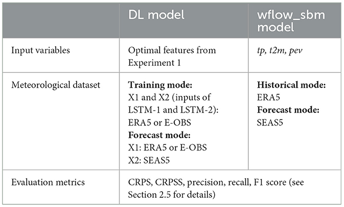
Table 2. Overview of the experimental setup for Experiment 2: operational forecast.
2.4.3 Experiment 3: fine-tuning using the SEAS5 dataset
The third experiment explores the flexibility of the DL approach by fine-tuning the pretrained model with limited SEAS5 dataset, aiming to make the most of the available data and evaluate its impact on the forecast performance. The DL model is first pre-trained using the ERA5 dataset. Subsequently, the LSTM-2 and Dense layers of the pre-trained model are fine-tuned, i.e., the trainable parameters of the layers are updated, using SEAS5 ensemble mean data. The fine-tuning employs a training subset from 2019-11-01 to 2022-04-01 and validation subset from 2017-10-01 to 2018-12-01, with a learning rate of 5e-5. This validation period is specially chosen to include the severe drought event in 2018. Other model layers are kept frozen. The fine-tuned model is then tested using SEAS5 ensembles from 2017-10-01 to 2018-12-01. The test results are compared to the ones from Experiment 2 without fine-tuning.
An overview of the experimental setup is provided in Table 3.
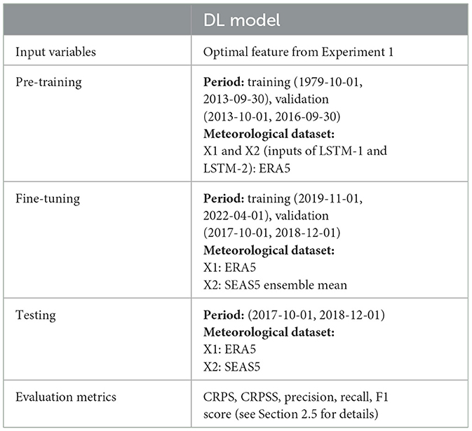
Table 3. Overview of the experimental setup for Experiment 3: fine-tuning using SEAS5.
2.5 Evaluation metrics
The evaluation specifically focuses on the results obtained during the low-flow season, which spans from April to September when low flows are most likely to occur at Lobith.
In the first experiment, the models are evaluated on the mean absolute error (MAE) and mean absolute percentage error (MAPE). MAE, in the same unit as the target (m3 s−1), offers a straightforward interpretation and is commonly used in deterministic forecast. This study involves varying discharge values across different seasons. MAPE, expressed in unit 100%, normalizes errors by expressing them as a percentage of the actual demand, which facilitates a more equitable comparison of forecasting performance across seasons. MAE and MAPE are more suitable for low flows, as they prevent larger errors, primarily associated with high flows, from disproportionately influencing the results, as is the case with MSE or RMSE due to their quadratic terms. In this study, MAE and MAPE are calculated for each time step (lead time) and averaged over the entire forecast time series within the dry season.
In the second and third experiments, the models are evaluated on the forecasts initialized during the dry season using the CRPS and compared with the benchmark using CRPSS. CRPS quantifies the dissimilarity between the cumulative density function of the ensemble forecast and the Heaviside function of the true observation. If there is only one predicted time series (deterministic prediction), the CRPS is equivalent to the MAE. The optimal value is 0, and the score increases with the increasing inaccuracy of the probabilistic forecast. The CRPS can serve as a Skill Score (CRPSS) by comparing it to a reference forecast. The CRPSS is calculated using Equation (1). If the model forecast is perfect, its CRPS will be 0, and the CRPSS with regard to reference forecast will become 1.0. If both forecasts demonstrate equal accuracy, the CRPSS will be 0. If the model forecast outperforms the reference forecast, the CRPSS will yield a positive value. Conversely, the CRPSS will be negative.
To evaluate the model performance on forecasting low-flow events during the second and third experiments, the metrics precision, recall and F1 score are used. For probabilistic forecasts, we firstly compute drought occurrence probabilities using the river discharge threshold outlined in Table 1. The drought occurrence probability is calculated as the ratio of predicted ensemble members that fall below the threshold value. Then, we classify the results into drought or non-drought. A threshold of 0.5 is applied to the drought occurrence probabilities. If the drought occurrence probability is equal or greater than 0.5, the result is classified as drought. If the drought occurrence probability is smaller than 0.5, the result is classified as non-drought. Finally, the precision, recall and F1 scores for different lead times are computed based on the forecasted binary classification (drought and non-drought) in comparison to the actual classification from observed discharges. Precision, also known as positive predictive value, is calculated as TP/(TP+FP). Recall, also referred to as hit rate or true positive rate, is calculated as TP/(TP+FN). TP stands for true positive, FP stands for false positive, and FN stands for false negative. F1 score is the harmonic mean of the precision and recall, thus representing both precision and recall in one metric. An F1 score of 1.0 indicates perfect precision and recall, and the lowest possible value is 0, if either precision or recall are zero.
3 Results and discussion
In this section, we first present the results and analysis of Experiment 1 on the selection of feature and target variables. This is followed by the results of Experiment 2, for which we investigate the capability of the DL model for operational forecast with SEAS5 and benchmark the DL model against the wflow_sbm hydrological model in forecasting low flows and drought events. Lastly, for Experiment 3, we examine whether the fine-tuned approach using SEAS5 enhances the forecast performance.
3.1 Feature and target selection
The first experiment explores different spatial resolutions of meteorological forcing, the use of different target variables, and the impact of incorporating historical discharge observations. Figure 4 shows the MAE and MAPE of test results from Experiment 1, using the E-OBS dataset and meteorological forcing as input variables on different combinations of spatial resolutions and target variables. The experiment results using the ERA5 dataset are presented in the Supplementary material.
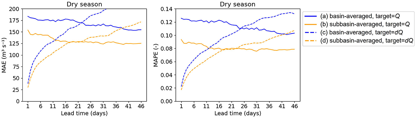
Figure 4. MAE and MAPE of Experiment 1 results using the E-OBS dataset and meteorological forcing as input variables on different combinations of spatial resolutions and target variables.
Comparing line (a) and (b), when using Q as target, the MAE of the subbasin-averaged approach decreases by approximately 25 m3 s−1 for all lead times compared to the basin-averaged approach. Comparing line (c) and (d), when using dQ as target, the MAE differences between the two approaches are minor for the first few lead times but keep increasing with an increasing lead time, i.e., the forecast horizon. Similar trends are obtained using the ERA5 dataset. The results indicate that using the subbasin-averaged approach for the meteorological forcing significantly improves the model performance regardless of the target variables. This aligns with expectations since the discharge at Lobith originates from different subbasins in different seasons, and a subbasin spatial resolution allows the model to capture the information from various subbasins at different times. In contrast, using the basin-averaged approach would obscure this crucial information. Also, when averaging to the whole basin, many precipitation rates, especially, become very low and irrelevant. This finding is consistent with previous studies (Troutman, 1983; Shah et al., 1996; Khakbaz et al., 2012) which have shown that considering the spatial variabilities of meteorological forcing, particularly precipitation, has a significant impact on the hydrologic response of basins.
Regarding the target variables, from Figure 4 we can see that employing dQ as target greatly improves the model performance for short lead times (1–6 days) compared to using Q as target, which is crucial for operational forecast as it ensures the forecast starts from an accurate state. However, after lead time = 21, the improvement provided by using dQ as a target variable diminishes for longer lead times due to error propagation along the forecast horizon, while the performance of using Q as target becomes stable for longer lead times. A similar trend is found using the ERA5 dataset, except that the MAE crossover point using different targets occurs earlier, around lead time = 11. For the application to real-world operations, we can leverage both approaches. For stakeholders involved in operational decision-making that prioritizes accurate short-term forecasts, emphasizing the use of dQ as the target variable ensures reliability and accuracy at the onset of the forecast horizon. On the other hand, for stakeholders involved in long-term planning, focusing on Q as the target variable provides a stable forecasting performance for extended lead times.
We also explored incorporating historical discharge at Lobith into LSTM-1 in the DL model. The experiment results, using the E-OBS dataset (Figure 5) and the ERA5 dataset (see Supplementary Figures 2, 3), show the positive impact of incorporating historical discharges (Q_his) on the overall model performance, regardless of the target variables used. From Figure 5, we can see that when using Q as target, the inclusion of historical discharges leads to a substantial improvement in model performance, particularly for short lead times. In contrast, when using dQ as a target variable, the improvement in performance is not as pronounced for short lead times (1–11 days), which shows the model's ability in forecasting low flows using only meteorological inputs. Nonetheless, as lead time increases, the benefit of incorporating Q_his becomes more evident. A comparison between line (e) and (f) in Figure 5 illustrates that, even when incorporating Q_his, using dQ as the target variable continues to outperform using Q as target for short lead times, and the performance gap between using dQ and Q as respective target variable diminishes as lead time increases.
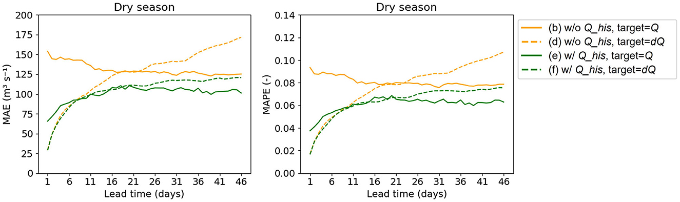
Figure 5. MAE and MAPE of Experiment 1 results using E-OBS dataset and subbasin-averaged approach on different combinations of input variables and target variables. Q_his stands for historical discharge observations. Lines (b) and (d) in this figure are taken from Figure 4.
It should be noted that in this experiment, we use a 270-day length, also called a lookback window, of historical discharge (Q_his) as an input variable, aligning it with the sequence length of the meteorological variables. The influence of using other lookback windows for this specific application has not been performed. Further investigation is necessary to understand the effect of varying Q_his lengths on model performance as it can help identify and prevent input redundancy.
In Experiment 1, two datasets are tested, i.e., E-OBS and ERA5, to explore their impacts on the model performance. From Figure 6, when using Q as target, the performances of models using E-OBS and ERA5 are comparable, regardless of whether Q_his is included in the inputs. The maximum MAE difference is around 25 m3 s−1. However, when using dQ as target, the performance of the model using the ERA5 dataset is notably inferior to that using E-OBS, especially for longer lead times, where the average MAE difference can reach beyond 30–50 m3 s−1. This observation suggests that dQ is more sensitive to the dataset used.
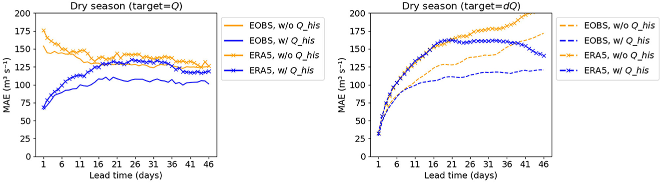
Figure 6. MAE of Experiment 1 results using different dataset, i.e., E-OBS and ERA5. The left figure presents the results using Q as target and a subbasin-averaged approach, while the right figure presents the results using dQ as target and a subbasin-averaged approach.
3.2 Operational forecast
The second experiment investigates the capability of the DL model for low-flow forecasting with SEAS5 data, benchmarked against the wflow_sbm model. Based on the findings of Experiment 1, we continue our analysis using DL models with subbasin-averaged meteorological forcing and Q_his as inputs, and dQ as target. If no further clarification is provided, the results shown in this section are using the ERA5 dataset for X1 (inputs of LSTM-1) and the SEAS5 dataset for X2 (inputs of LSTM-2.
The example presented in Figure 7 demonstrates the forecast results of the DL model and wflow_sbm model with SEAS5 initialized on 2018-08-01. In this forecast, the DL model exhibits a strong performance in predicting this low-flow event. The forecast of the DL model begins with an accurate initial state, resulting in well-predicted discharge values for the first 6 days compared to the observed data. The median values closely align with the observed values throughout the entire forecast horizon. And all 46 observations fall within the 33–66% band of the DL model forecasts. In contrast, for the wflow_sbm model, the initial state is not corrected using near real time observations leading to an initial offset from the ground truth in the first few days. As the lead time increases, the wflow_sbm model tends to underestimate the discharge, thereby overestimating the severity of the drought conditions.
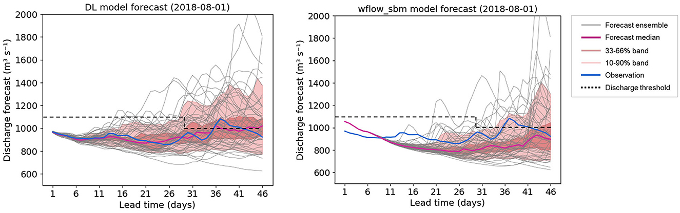
Figure 7. Forecast results of the DL model and the wflow_sbm model with SEAS5 initialized on 2018-08-01.
The forecast results initialized during the dry season are evaluated using CRPS. The DL model exhibits lower CRPS values compared to the wflow_sbm model for both short and long lead times, indicating higher forecast accuracy (see Supplementary Figure 4). To facilitate the comparison, the CRPSS of the DL model is computed relative to the wflow_sbm forecast results and shown in Figure 8. The median values for all lead times are above zero, indicating that the DL model exhibits skill in forecasting discharge during the dry season, with improved performance over the wflow_sbm model.
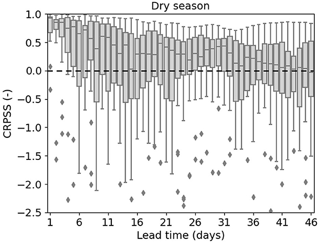
Figure 8. CRPSS of the DL model forecasts compared to the wflow_sbm model forecasts. The dashed line indicates the CRPSS value of zero.
The discharge forecast results are post-processed into drought occurrence probability using the river discharge threshold in Table 1, based on which the forecasted event classifications (drought or non-drought) are obtained. Figure 9 shows an example forecast result of drought occurrence probability initialized on 2018-08-01. Within a lead time of up to 31 days, both the DL model and the wflow_sbm model accurately predict drought events, even though the drought occurrence probabilities from the wflow_sbm model are slightly higher than those from the DL model. However, for lead times after 31 days, both models struggle to classify the event between lead times 36–41 days.
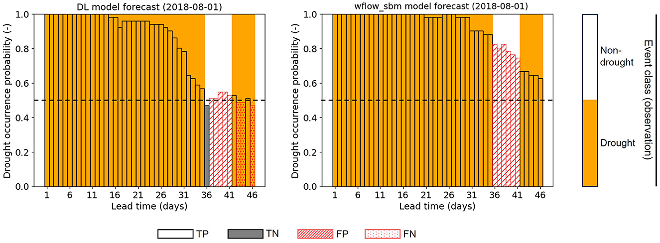
Figure 9. Drought forecasting results (drought occurrence probabilities and classifications) of the DL model and the wflow_sbm model with SEAS5 initialized on 2018-08-01. The dashed line indicates the threshold of 0.5 applied to the drought occurrence probabilities. The observed event classes (drought or non-drought) are provided with the background orange bar color.
Figure 10 presents the F1 score of drought forecasting results from the DL model and the wflow_sbm model across different lead times. The results of precision and recall values can be found in Supplementary Figure 5. In the initial lead times (1–11 days), the DL model has higher F1 scores compared to the wflow_sbm model which as mentioned before does not have initial state update using near real time observations. This suggests that the DL model exhibits better accuracy in forecasting drought events within short lead times. For lead times 11-21 days, the F1 scores of the wflow_sbm model are equal or higher than those of the DL model. In the subsequent lead times 21–31 days, the DL model maintains slightly higher F1 scores. But for lead times after 31 days, the wflow_sbm model has higher scores.
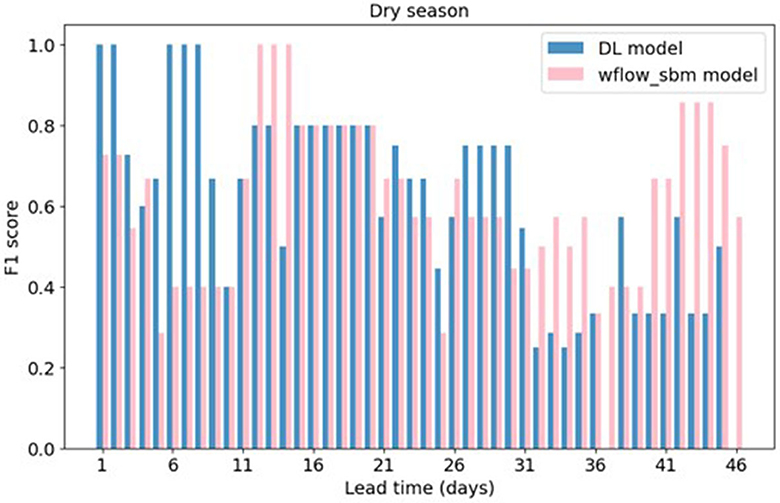
Figure 10. F1 score of drought forecasting results from the DL model and the wflow_sbm model with SEAS5.
In this experiment, the comparison between the DL model and the wflow_sbm model might not have been conducted under the most optimal conditions for the two models. This is because the wflow_sbm model used in this comparison does not have any state update mechanism, potentially causing it to initiate from an incorrect initial state. This discrepancy could have influenced its performance across the entire forecast horizon. If the wflow_sbm results were corrected for this initial bias, it potentially would provide a stronger basis for benchmarking the DL model.
Furthermore, the DL model is trained on data from the year 1979 to 2016, and the trained model is then used for all forecasts. However, for operational use, it is preferable to train the model using as much data as possible prior to initialization. Different training strategies could impact the forecast skill of the DL model, and it is hypothesized that utilizing more training data can improve its performance in the forecast mode. Although this study does not explore this aspect, it presents an opportunity for future improvements.
Another crucial point to discuss is the choice of data sources in this experiment. During training, ERA5 is used for both LSTMs in the model, while in the forecast mode, ERA5 is used for X1 (inputs of LSTM-1) along with SEAS5 for X2 (inputs of LSTM-2). SEAS5 data is not used for training due to the limited number of samples available. Although this setup leaves the forecast mode vulnerable to biases present in SEAS5, this might be mitigated to some extent since ERA5 and SEAS5 are both generated using the atmospheric model ECMWF Integrated Forecast System (IFS). Additionally, using SEAS5 in the forecast mode allows for testing the robustness of the DL model when utilizing a different dataset from the training phase. The same experiment is conducted using E-OBS instead of ERA5. The results of using E-OBS (Supplementary Figure 6) indicate a deterioration in the DL model's performance compared to the experiment with ERA5 (Figure 8), especially for lead times beyond 31 days. This underscores the importance of using same or similar data sources for both training and forecasting phases.
In terms of computational efficiency in this experiment, it is worth mentioning that, in forecast mode, the DL model's runtime for one forecast result is around 2 s including pre- and post-processing when using Google Colab with a T4 GPU, while the wflow_sbm model runtime is around 2 h for one forecast result with a 7-month lead time using CPU. However, the DL model only predicts a single variable at a specific location, whereas the wflow_sbm model generates multiple variables for every model grid cell.
3.3 Effect of fine-tuning
As mentioned in the precious experiment, SEAS5 data is not used for training due to the limited data available. The third experiment explores the flexibility of the DL approach by fine-tuning the pretrained model with limited SEAS5 dataset, aiming to make the most of the available data and evaluate its impact on the forecast performance. The experiment employs the same setup of Experiment 2, utilizing the same feature and target variables. The historical meteorological inputs are from the ERA5 dataset. The fine-tuned model is tested using SEAS5 ensembles from 2017-10-01 to 2018-12-01. In total, there are 15 forecast results, 6 of which are initialized during the dry season from April to September.
The test results from the fine-tuned model are evaluated against the non-fine-tuned model on the same period using CRPSS (Figure 11). The median CRPSS values for lead times from 2 to 18 days indicate small improvement attributed to fine-tuning. Nevertheless, the median values for lead times beyond 18 days fall slightly below zero, suggesting that fine-tuning brings about a slight degradation rather than enhancement in forecasting skill for longer lead times.
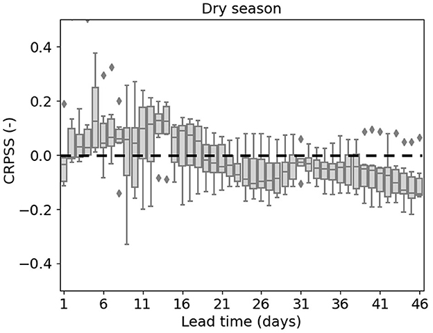
Figure 11. CRPSS of the fine-tuned DL model forecasts compared to the non-fine-tuned DL model. The dashed line indicates the CRPSS value of zero.
The F1 score of drought forecasting results from the fine-tuned model and the non-fine-tuned model are shown in Figure 12. The precision and recall results can be found in Supplementary Figure 7. For lead times from 1 to 31 days, the F1 score of the two models exhibit close alignment. Notably, the fine-tuned model demonstrates higher precision for certain lead times, while the non-fine-tuned model shows higher recall for specific lead times. Nevertheless, for lead times beyond 31 days, the fine-tuned model registers zero F1 scores, in contrast to the non-fine-tuned model which maintains non-zero scores. This discrepancy suggests that the fine-tuned model encounters difficulty in forecasting drought events for longer lead times.
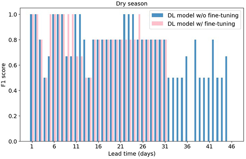
Figure 12. F1 score of drought forecasting results from the DL with and without fine-tuning.
The fine-tuning using SEAS5 ensemble mean appears to worsen the forecast performance for lead times beyond 31 days. One plausible explanation for this phenomenon could be attributed to the use of the ensemble mean forecasted data for fine-tuning. The meteorological forecast ensembles exhibit limited spread during the initial lead times, for which the ensemble mean serve as an estimate of the expected values for each ensemble. However, as the lead time increases, the meteorological forecast ensemble variability increases significantly, making the ensemble mean insufficient to represent the full spectrum of forecast probabilities. Furthermore, we use a relatively small dataset for the fine-tuning process. Consequently, the utilization of the limited ensemble mean dataset for fine-tuning might inadvertently introduce biases into the model predictions.
The experiment involves a relatively small sample of the SEAS5 dataset. A total of 30 samples are allocated for training and 15 samples for validation, leaving only 15 samples available for testing. Moreover, to establish a validation dataset, the ensemble means of the 15 validation samples overlapping with the testing period are employed during the fine-tuning process. Despite the limited dataset, the experiment findings underscore the influence of fine-tuning on model performance.
4 Limitations and future works
This study aims to explore the potential of LSTMs for low-flow forecasting for the Rhine River at Lobith with a lead time of up to 46 days. Based on the results and discussions, several limitations of this study are identified, along with recommendations for improvement and future research.
Regarding the input data, the study utilizes three meteorological variables – total precipitation (tp), 2-meter temperature (t2m), and potential evaporation (pev) – to describe the meteorological conditions over time. However, the influences of these variables on the DL models are not studied. It is therefore suggested to conduct a SHAP (SHapley Additive exPlanations) analysis (Lundberg and Lee, 2017) to assess how these three variables impact the model results. Furthermore, future studies might explore the integration of a broader set of variables from sources such as ERA5 or E-OBS.
In addition to the historical discharges utilized in this study, other hydrological variables such as snow melt, soil moisture or water levels from Lake Constance or information on reservoir operations might be valuable to explore as input to the DL model, given that the water storage in snowpack and large lakes particularly in Switzerland influence the contribution of discharge at Lobith during dry periods (Demirel et al., 2013).
Regarding the choice of a loss function, the study uses the mean squared error (MSE), which is commonly employed in the DL models. However, it is recommended to explore alternative objective functions that are suitable for time series forecasting of non-stationary signals and multiple future steps prediction. One promising alternative is the DILATE function developed by Le Guen and Thome (2019). The DILATE function aims to accurately predict sudden changes and incorporates terms that facilitate precise shape and temporal change detection. This loss function would be beneficial for predicting the timing, specifically the start and end of drought events in this study. Additionally, in the case of using dQ as the target variable, it might be beneficial to explore a directional loss function, which has the potential to guide the model in focusing on not only the magnitude but also the direction of changes.
In Experiment 1 – feature and target selection, it has been found that the best performance is obtained when using dQ as the target variable, along with tp, t2m, pev, and Q_his as input variables. This finding specifically applies to the Rhine River at Lobith, where long-term continuously measured discharges are available. However, for predictions in ungauged basins where observed discharges are lacking, only general meteorological forcing (e.g., tp, t2m, pev) may be accessible. As a result, there is potential to investigate the viability of forecasting ungauged basins through transfer learning. This involves training a rainfall-runoff model on large-sample dataset with only meteorological variables as inputs, thereby contributing to a broader applicability of the developed model.
Regarding the fine-tuning approach, it would be valuable to explore with more SEAS5 data. Also, instead of using the forecasted ensemble mean, incorporating various time series outputs from the ensembles, such as the minimum, 25th percentile, median, 75th percentile and maximum, could yield worthwhile insights and improvements.
For the application of the DL model in real-world operations, it is important to provide a prediction interval that captures the uncertainty of the predicted values. It is recommended that this be included in future works. Also, adapting the model for hourly time steps and training with meteorological datasets used in operation can be valuable for smaller catchments.
5 Conclusion
This research explores the potential of using LSTMs for low-flow forecasting for the Rhine River at Lobith on a daily scale with lead times up to 46 days ahead. A novel LSTM-based model architecture is designed to leverage both historical observations and forecasted meteorological data to carry out multi-step discharge time series forecasting.
The investigation into feature and target selection yields the following key insights: (1) Opting for subbasin-averaged meteorological variables significantly improves model performance compared to a basin-averaged approach. (2) Utilizing time-differenced data (dQ) as the target boosts short-term forecast accuracy compared to Q, but this advantage diminishes after a lead time of 20 days due to error propagation. In contrast, using Q as the target variable results in a stable performance for longer lead times. (3) While incorporating historical discharge improves the forecasting of Q, its impact on predicting dQ is less pronounced for short lead times, highlighting the model's ability in generating accurate forecasts using only meteorological inputs.
In the operational forecast with SEAS5, the DL model exhibits skill in forecasting low flows, with improved performance over the benchmark wflow_sbm model, as evidenced by CRPSS median values of all lead times above zero. The assessment of drought forecasting precision and recall reveals that the DL model exhibits better accuracy in forecasting drought events within short lead times. The wflow_sbm model shows higher accuracy for longer lead times. From operational perspective the point DL model is significantly faster than the wflow_sbm model, although the wflow_sbm model provides multiple modeled state variables for each grid cell.
In exploring the fine-tuning approach with the SEAS5 dataset, the fine-tuning makes small improvement over non-fine-tuned model for short lead times, but encounters difficulty in forecasting drought events for longer lead times. Despite the limited dataset, the experiment underscores the influence of fine-tuning on model performance. For future research, it would be valuable to explore the fine-tuning approach with more SEAS5 data and incorporating various time series outputs from the ensembles.
Compared to the previous studies on forecasting low flows for the Rhine River for longer lead times (e.g., Demirel et al., 2013; Yossef et al., 2013; Klein and Meißner, 2018; Hurkmans et al., 2023), the DL model in this study shows skills for forecasting low flows with lead times up to 5–6 weeks, not only during the spring and early summer periods but also extending to the late summer and early autumn periods.
Overall, this study contributes to advancing the field of low-flow forecasting using a deep learning approach. Future research could explore additional improvements to the model performance, investigate the viability of forecasting ungauged basins through transfer learning, add prediction intervals for each lead time, and adapt for hourly time steps for smaller catchments.
Data availability statement
The original contributions presented in the study are included in the article/Supplementary material, further inquiries can be directed to the corresponding author.
Author contributions
JD: Conceptualization, Methodology, Project administration, Software, Validation, Visualization, Writing—original draft, Writing—review & editing. AC: Conceptualization, Methodology, Resources, Supervision, Writing—review & editing. RD: Conceptualization, Methodology, Project administration, Resources, Supervision, Writing—review & editing. MH: Conceptualization, Methodology, Writing—review & editing. K-JvH: Conceptualization, Methodology, Writing—review & editing. HK: Conceptualization, Methodology, Writing—review & editing. AW: Resources, Writing—review & editing. RT: Conceptualization, Methodology, Supervision, Writing—review & editing.
Funding
The author(s) declare that no financial support was received for the research, authorship, and/or publication of this article.
Acknowledgments
This manuscript is based on the Master of Science thesis of Deng (2023). We thank Maarten Verbrugge for the work on bias correction of SEAS5 dataset used in this study. We are grateful to the reviewers for their constructive feedback and insightful suggestions.
Conflict of interest
The authors declare that the research was conducted in the absence of any commercial or financial relationships that could be construed as a potential conflict of interest.
Publisher's note
All claims expressed in this article are solely those of the authors and do not necessarily represent those of their affiliated organizations, or those of the publisher, the editors and the reviewers. Any product that may be evaluated in this article, or claim that may be made by its manufacturer, is not guaranteed or endorsed by the publisher.
Supplementary material
The Supplementary Material for this article can be found online at: https://www.frontiersin.org/articles/10.3389/frwa.2023.1332678/full#supplementary-material
Footnotes
References
Aghelpour, P., Bahrami-Pichaghchi, H., and Varshavian, V. (2021). Hydrological drought forecasting using multi-scalar streamflow drought index, stochastic models and machine learning approaches, in northern Iran. Stochastic Environ. Res. Risk Assessm. 35, 1615–1635. doi: 10.1007/s00477-020-01949-z
Amanambu, A. C., Mossa, J., and Chen, Y. H. (2022). Hydrological drought forecasting using a deep transformer model. Water 14, 3611. doi: 10.3390/w14223611
Borji, M., Malekian, A., Salajegheh, A., and Ghadimi, M. (2016). Multi-time-scale analysis of hydrological drought forecasting using support vector regression (SVR) and artificial neural networks (ANN). Arab. J. Geosci. 9, 725. doi: 10.1007/s12517-016-2750-x
Cammalleri, C., Naumann, G., Mentaschi, L., Bisselink, B., Gelati, E., De Roo, A., et al. (2020). Diverging hydrological drought traits over Europe with global warming. Hydrol. Earth Syst. Sci. 24, 5919–5935. doi: 10.5194/hess-24-5919-2020
Cornes, R. C., van der Schrier, G., van den Besselaar, E. J. M., and Jones, P. D. (2018). An ensemble version of the E-OBS temperature and precipitation data sets. J. Geophys. Res. Atmospheres 123, 9391–9409. doi: 10.1029/2017JD028200
De Vries, D., Kort, H., Teunis, B., Winters, B. M., and Beijk, V. (2021). Landelijk Draaiboek Waterverdeling en Droogte. Available online at: www.helpdeskwater.nl (accessed December 5, 2022).
Demirel, M. C., Booij, M. J., and Hoekstra, A. Y. (2013). Identification of appropriate lags and temporal resolutions for low flow indicators in the River Rhine to forecast low flows with different lead times. Hydrol. Process 27, 2742–2758. doi: 10.1002/hyp.9402
Deng, J. (2023). Operational Streamflow Drought Forecasting for the Rhine River at Lobith Using the LSTM Deep Learning Approach. Available online at: http://resolver.tudelft.nl/uuid:331a6ac2-0ba9-4726-8672-003cf762ad60 (accessed October 23, 2023).
Dikshit, A., Pradhan, B., and Santosh, M. (2022). Artificial neural networks in drought prediction in the 21st century–A scientometric analysis. Appl. Soft. Comput. 114, 108080. doi: 10.1016/j.asoc.2021.108080
EEA (2010). Mapping the Impacts of Natural Hazards and Technological Accidents in Europe An Overview of the Last Decade. Copenhagen: EEA.
Fang, K., Shen, C., Kifer, D., and Yang, X. (2017). Prolongation of SMAP to spatiotemporally seamless coverage of continental U.S. using a deep learning neural network. Geophys. Res. Lett. 44, 11–30. doi: 10.1002/2017GL075619
Frame, J. M., Kratzert, F., Klotz, D., Gauch, M., Shalev, G., Gilon, O., et al. (2022). Deep learning rainfall–runoff predictions of extreme events. Hydrol. Earth Syst. Sci. 26, 3377–3392. doi: 10.5194/hess-26-3377-2022
Franken, T., Gullentops, C., Wolfs, V., Defloor, W., Cabus, P., Jongh, D., et al. (2022). An operational framework for data driven low flow forecasts in Flanders. EGU Gen. Assemb. Conf. Abstr. 12, EGU22–6191. doi: 10.5194/egusphere-egu22-6191
Gauch, M., Kratzert, F., Klotz, D., Nearing, G., Lin, J., Hochreiter, S., et al. (2021). Rainfall–runoff prediction at multiple timescales with a single long short-term memory network. Hydrol. Earth Syst. Sci. 25, 2045–2062. doi: 10.5194/hess-25-2045-2021
Hauswirth, S. M., Bierkens, M. F. P., Beijk, V., and Wanders, N. (2023). The suitability of a seasonal ensemble hybrid framework including data-driven approaches for hydrological forecasting. Hydrol. Earth Syst. Sci. 27, 501–517. doi: 10.5194/hess-27-501-2023
Hersbach, H., Bell, B., Berrisford, P., Biavati, G., Horányi, A., Muñoz Sabater, J., et al. (2023). ERA5 Hourly Data on Single Levels From 1940 to Present. London: ECMWF.
Hunt, K. M. R., Matthews, G. R., Pappenberger, F., and Prudhomme, C. (2022). Using a long short-term memory (LSTM) neural network to boost river streamflow forecasts over the western United States. Hydrol. Earth Syst. Sci. 26, 5449–5472. doi: 10.5194/hess-26-5449-2022
Hurkmans, R. T. W. L., van den Hurk, B., Schmeits, M., Wetterhall, F., and Pechlivanidis, I. G. (2023). Seasonal streamflow forecasting for fresh water reservoir management in the netherlands: an assessment of multiple prediction systems. J. Hydrometeorol. 24, 1275–1290. doi: 10.1175/JHM-D-22-0107.1
Imhoff, R. O., van Verseveld, W. J., van Osnabrugge, B., and Weerts, A. H. (2020). Scaling point-scale (pedo)transfer functions to seamless large-domain parameter estimates for high-resolution distributed hydrologic modeling: an example for the rhine river. Water Resour. Res. 56, e2019WR026807. doi: 10.1029/2019WR026807
International Commission for the Protection of the Rhine (2018). Inventory of the Low Water Conditions on the Rhine. Available online at: www.iksr.org (accessed May 10, 2023).
Ionita, M., Tallaksen, L. M., Kingston, D. G., Stagge, J. H., Laaha, G., Van Lanen, H. A. J., et al. (2017). The European 2015 drought from a climatological perspective. Hydrol. Earth Syst. Sci. 21, 1397–1419. doi: 10.5194/hess-21-1397-2017
Johnson, S. J. (2019). SEAS5: The new ECMWF seasonal forecast system. Geosci. Model Dev. 12, 1087–1117. doi: 10.5194/gmd-12-1087-2019
Kao, I. F., Zhou, Y., Chang, L. C., and Chang, F. J. (2020). Exploring a long short-term memory based encoder-decoder framework for multi-step-ahead flood forecasting. J. Hydrol. 583, 124631. doi: 10.1016/j.jhydrol.2020.124631
Khakbaz, B., Imam, B., Hsu, K., and Sorooshian, S. (2012). From lumped to distributed via semi-distributed: Calibration strategies for semi-distributed hydrologic models. J. Hydrol. 419, 61–77. doi: 10.1016/j.jhydrol.2009.02.021
Klein, B., and Meißner, D. (2018). Impact of Hydrological Model Uncertainty on Predictability of Seasonal Streamflow Forecasting in the River Rhine Basin. Available online at: https://hepex.org.au/wp-content/uploads/2018/02/1450-1510-Klein-Impact-of-model-uncertainty-on-predictability.pdf (accessed September 12, 2023).
Kramer, N., Mens, M., Beersma, J., and Kielen, N. (2019). Hoe extreem was de droogte van 2018? Available online at: https://www.h2owaternetwerk.nl/vakartikelen/hoe-extreem-was-de-droogte-van-2018 (accessed December 27, 2022).
Kratzert, F., Klotz, D., Brenner, C., Schulz, K., and Herrnegger, M. (2018). Rainfall–runoff modelling using long short-term memory (LSTM) networks. Hydrol. Earth Syst. Sci. 22, 6005–6022. doi: 10.5194/hess-22-6005-2018
Kratzert, F., Klotz, D., Herrnegger, M., Sampson, A. K., Hochreiter, S., Nearing, G. S., et al. (2019a). Toward improved predictions in ungauged basins: exploiting the power of machine learning. Water Resour. Res. 55, 11344–11354. doi: 10.1029/2019WR026065
Kratzert, F., Klotz, D., Shalev, G., Klambauer, G., Hochreiter, S., Nearing, G., et al. (2019b). Towards learning universal, regional, and local hydrological behaviors via machine learning applied to large-sample datasets. Hydrol Earth Syst. Sci. 23, 5089–5110. doi: 10.5194/hess-23-5089-2019
Le Guen, V., and Thome, N. (2019). Shape and time distortion loss for training deep time series forecasting models. Adv. Neural Inf. Process Syst. 32. doi: 10.48550/arXiv.1909.09020
Lundberg, S. M., and Lee, S. I. (2017). A unified approach to interpreting model predictions. Adv. Neural. Inf. Process Syst. 30, 1–5. doi: 10.48550/arXiv.1705.07874
Middelkoop, H., and van Haselen, C. (1999). Twice a River Rhine and Meuse in the Netherlands. RIZA Report 99.003. Utrecht: Institute for Inland Water Management and Waste Water Treatment (RIZA).
Mosavi, A., Ozturk, P., and Chau, K. (2018). Flood prediction using machine learning models: literature review. Water 10:1536. doi: 10.3390/w10111536
Nearing, G., Cohen, D., Dube, V., Gauch, M., Gilon, O., Harrigan, S., et al. (2023). AI increases global access to reliable flood forecasts. arXiv [Preprint]. arXiv: 2307.16104. doi: 10.48550/arXiv.2307.16104
Nevo, S., Morin, E., Gerzi Rosenthal, A., Metzger, A., Barshai, C., Weitzner, D., et al. (2022). Flood forecasting with machine learning models in an operational framework. Hydrol Earth Syst Sci 26, 4013–4032. doi: 10.5194/hess-26-4013-2022
Prudhomme, C., Giuntoli, I., Robinson, E. L., Clark, D. B., Arnell, N. W., Dankers, R., et al. (2014). Hydrological droughts in the 21st century, hotspots and uncertainties from a global multimodel ensemble experiment. Proc. Natl. Acad. Sci. U. S. A. 111, 3262–3267. doi: 10.1073/pnas.1222473110
Rijkswaterstaat (2019). Water Management in the Netherlands. Available online at: http://www.helpdeskwater.nl/watermanagement (accessed December 17, 2022).
Sahoo, B. B., Jha, R., Singh, A., and Kumar, D. (2019). Long short-term memory (LSTM) recurrent neural network for low-flow hydrological time series forecasting. Acta Geophysica 67, 1471–1481. doi: 10.1007/s11600-019-00330-1
Shah, S. M. S., O'Connell, P. E., and Hosking, J. R. M. (1996). Modelling the effects of spatial variability in rainfall on catchment response. 2. Experiments with distributed and lumped models. J. Hydrol. 175, 89–111. doi: 10.1016/S0022-1694(96)80007-2
Shamshirband, S., Hashemi, S., Salimi, H., Samadianfard, S., Asadi, E., Shadkani, S., et al. (2020). Predicting standardized streamflow index for hydrological drought using machine learning models. Eng. Appl. Comput. Fluid Mech. 14, 339–350. doi: 10.1080/19942060.2020.1715844
Shen, C. (2018). A transdisciplinary review of deep learning research and its relevance for water resources scientists. Water Resour. Res. 54, 8558–8593. doi: 10.1029/2018WR022643
Shen, C., Chen, X., and Laloy, E. (2021). Editorial: broadening the use of machine learning in hydrology. Frontiers in Water 3, 681023. doi: 10.3389/frwa.2021.681023
Switanek, M. B., Troch, P. A., Castro, C. L., Leuprecht, A., Chang, H.-. I, Mukherjee, R., et al. (2017). Scaled distribution mapping: a bias correction method that preserves raw climate model projected changes. Hydrol. Earth Syst. Sci. 21, 2649–2666. doi: 10.5194/hess-21-2649-2017
Tallaksen, L. M., and Van Lanen, H. (2004). Hydrological Drought: Processes and Estimation Methods for Streamflow and Groundwater. Elsevier: Developments in Water Science.
Troutman, B. M. (1983). Runoff prediction errors and bias in parameter estimation induced by spatial variability of precipitation. Water Resour. Res. 19, 791–810. doi: 10.1029/WR019i003p00791
van der Wiel, K., Wanders, N., Selten, F. M., and Bierkens, M. F. P. (2019). Added Value of Large Ensemble Simulations for Assessing Extreme River Discharge in a 2 °C Warmer World. Geophys Res Lett 46, 2093–2102. doi: 10.1029/2019GL081967
Van Lanen, H. A. J., Wanders, N., Tallaksen, L. M., and Van Loon, A. F. (2013). Hydrological drought across the world: impact of climate and physical catchment structure. Hydrol. Earth Syst. Sci. 17, 1715–1732. doi: 10.5194/hess-17-1715-2013
Van Loon, A. F. (2015). Hydrological drought explained. WIREs Water 2, 359–392. doi: 10.1002/wat2.1085
Van Loon, A. F., Gleeson, T., Clark, J., Van Dijk, A. I. J. M., Stahl, K., Hannaford, J., et al. (2016). Drought in the Anthropocene. Nat. Geosci. 9, 89–91. doi: 10.1038/ngeo2646
Van Loon, A. F., and Van Lanen, H. A. J. (2012). A process-based typology of hydrological drought. Hydrol. Earth Syst. Sci. 16, 1915–1946. doi: 10.5194/hess-16-1915-2012
van Osnabrugge, B., Uijlenhoet, R., and Weerts, A. (2019). Contribution of potential evaporation forecasts to 10-day streamflow forecast skill for the Rhine River. Hydrol. Earth Syst. Sci. 23, 1453–1467. doi: 10.5194/hess-23-1453-2019
van Verseveld, W. J., Weerts, A. H., Visser, M., Buitink, J., Imhoff, R. O., Boisgontier, H., et al. (2022). Wflow_sbm v0.6.1, a spatially distributed hydrologic model: from global data to local applications. Geosci. Model Dev. Disc. 2022, 1–52. doi: 10.5194/gmd-2022-182
Wanders, N., and Van Lanen, H. A. J. (2015). Future discharge drought across climate regions around the world modelled with a synthetic hydrological modelling approach forced by three general circulation models. Nat. Hazards Earth Syst. Sci. 15, 487–504. doi: 10.5194/nhess-15-487-2015
Wang, Z., Wang, Z., Long, Y., Wang, J., Xu, Z., Wang, B., et al. (2019). Enhancing generative conversational service agents with dialog history and external knowledge. Comput. Speech Lang. 54, 71–85. doi: 10.1016/j.csl.2018.09.003
Weerts, A. (2009). Improving Operational Flood Forecasting Through Data Assimilation. Available online at: https://publications.deltares.nl/1200379_005.pdf (accessed April 11, 2009).
Wilbrand, K., Taormina, R., ten Veldhuis, M.-C., Visser, M., Hrachowitz, M., Nuttall, J., et al. (2023). Predicting streamflow with LSTM networks using global datasets. Front. Water 5, 1166124. doi: 10.3389/frwa.2023.1166124
Wilhite, D., and Glantz, M. (1985). Understanding: the drought phenomenon: the role of definitions. Water Int. 10, 111–120. doi: 10.1080/02508068508686328
Keywords: low flow, operational forecasting, LSTM, deep learning, Rhine River, Lobith
Citation: Deng J, Couasnon A, Dahm R, Hrachowitz M, van Heeringen KJ, Korving H, Weerts A and Taormina R (2024) Operational low-flow forecasting using LSTMs. Front. Water 5:1332678. doi: 10.3389/frwa.2023.1332678
Received: 03 November 2023; Accepted: 29 December 2023;
Published: 17 January 2024.
Edited by:
Matteo Giuliani, Polytechnic University of Milan, ItalyReviewed by:
Claudia Bertini, IHE Delft Institute for Water Education, NetherlandsMatteo Sangiorgio, Polytechnic University of Milan, Italy
Wenjin Hao, Polytechnic University of Milan, Italy, in collaboration with reviewer MS
Copyright © 2024 Deng, Couasnon, Dahm, Hrachowitz, van Heeringen, Korving, Weerts and Taormina. This is an open-access article distributed under the terms of the Creative Commons Attribution License (CC BY). The use, distribution or reproduction in other forums is permitted, provided the original author(s) and the copyright owner(s) are credited and that the original publication in this journal is cited, in accordance with accepted academic practice. No use, distribution or reproduction is permitted which does not comply with these terms.
*Correspondence: Jing Deng, jing.deng@deltares.nl