 Ghazal Shabestanipour1
 Zachary Brodeur2
 Benjamin Manoli1Abigail Birnbaum1
 Scott Steinschneider2
 Jonathan R. Lamontagne1*
- 1Department of Civil and Environmental Engineering, Tufts University, Medford, MA, United States
- 2Department of Biological and Environmental Engineering, Cornell University, Ithaca, NY, United States
Water resources planning and management requires the estimation of extreme design events. Anticipated climate change is playing an increasingly prominent role in the planning and design of long-lived infrastructure, as changes to climate forcings are expected to alter the distribution of extremes in ways and to extents that are difficult to predict. One approach is to use climate projections to force hydrologic models, but this raises two challenges. First, global climate models generally focus on much larger scales than are relevant to hydrologic design, and regional climate models that better capture small scale dynamics are too computationally expensive for large ensemble analyses. Second, hydrologic models systematically misrepresent the variance and higher moments of streamflow response to climate, resulting in a mischaracterization of the extreme flows of most interest. To address both issues, we propose a new framework for non-stationary risk-based hydrologic design that combines a stochastic weather generator (SWG) that accurately replicates basin-scale weather and a stochastic watershed model (SWM) that accurately represents the distribution of extreme flows. The joint SWG-SWM framework can generate large ensembles of future hydrologic simulations under varying climate conditions, from which design statistics and their uncertainties can be estimated. The SWG-SWM framework is demonstrated for the Squannacook River in the Northeast United States. Standard approaches to design flows, like the T-year flood, are difficult to interpret under non-stationarity, but the SWG-SWM simulations can readily be adapted to risk and reliability metrics which bare the same interpretation under stationary and non-stationary conditions. As an example, we provide an analysis comparing the use of risk and more traditional T-year design events, and conclude that risk-based metrics have the potential to reduce regret of over- and under-design compared to traditional return-period based analyses.
1 Introduction
Water resources infrastructure is generally designed to manage hydrologic extremes. Conventionally, such designs have leveraged historical extreme events to estimate the magnitude of future extremes associated with some annual exceedance probability (AEP). For instance, design floods and design storms associated with different return periods are commonly used to size infrastructure (Haghighatafshar et al., 2020), and such analyses form the basis of standard design criteria in many countries (e.g., Bulletin 17C). Here, a flood or storm magnitude associated with the T-year return period (or recurrence interval) is an event with a p = 1/T AEP (Gumbel, 1941). The terms ‘return period’ and ‘recurrence interval’ arise because is the average time until a -year event is exceeded, assuming the events are independent and stationary (Stedinger et al., 1993).
However, climate change complicates water resources planning in general, and the use of design events and return periods in particular. Human-induced climate change is expected to have various impacts on atmospheric and hydrologic systems, such as intensified and intermittent precipitation (IPCC, 2023), changes in snow accumulation and timing, unprecedented rates of snow and glacier melt (Pörtner et al., 2022), sea level rise (Oki and Kanae, 2006), and longer droughts and dry periods due to increased potential evapotranspiration and decline in soil moisture (Balting et al., 2021), among others. These climate impacts are expected to alter the distribution of hydrologic extremes over time as the Earth continues to warm. Mapping changes in climate drivers to changes in hydrologic extremes is challenging because of the complicated and nonlinear nature of the hydrologic cycle and the path dependence of extreme events (Vogel, 2017).
Even if it is possible to estimate the evolution of non-stationary hydrologic extremes, Read and Vogel (2015) raised several concerns with the use of return periods and AEPs in hydrologic design in a non-stationary world. First, the interpretation of a return period is ambiguous when the AEP associated with a design flow is changing over time, and alternative definitions have been proposed. Read and Vogel (2015) show that the mean and distribution of the actual return period of a design event changes substantially as a function of the long-term trend in the annual maximum series, its variability, and the severity of the design event. If the annual maximum series is increasing over time, the relative reduction in the true return period of a design flow increases with the extremity of the design flow. For example, the true return period of the stationary 100-year flood will decrease relatively more than the true return period of the stationary 10-year flood.
Fernández and Salas (1999) Pielke (1999), and Read and Vogel (2015) have also critiqued the use of return periods and AEPs in design under stationary conditions. In addition to a general misunderstanding of their meaning by practitioners and the public alike (Fernández and Salas, 1999; Pielke, 1999; Douglas et al., 2002; Cooley, 2012; Serinaldi, 2015; Serinaldi and Kilsby, 2015), return periods and AEPs do not account for the design-life of the structure (Haghighatafshar et al., 2020), and so do not directly relate the risk-of-failure or reliability of a design over its intended design life. The lifetime risk of failure is likely of more use to planners and engineers than the average return period or 1 year AEP. This problem only compounds when the likelihood of extremes changes over time under climate change.
An alternative approach for water resources infrastructure design that is more suitable under non-stationarity is design-life specific risk or reliability. Here risk is defined as the probability a critical threshold is exceeded over the design-life, and reliability is the probability the critical threshold is not exceeded (reliability = 1-risk). Thus, the calculation is tailored toward the question: how likely is it that a project will fail over a T-year planning horizon? Engineers can then size, design, and manage infrastructure to meet a pre-selected level of risk deemed acceptable. Even if the probability of extremes evolves over the planning horizon, as is expected under climate change, the risk of project failure can still be presented as a single design value, assuming the time-varying distribution of extremes is integrated into the calculation of risk. This is in contrast to the traditional planning approaches that use design events for specific return periods. Return periods do not account for climate change dynamic impacts on hydrologic processes that govern extreme events. Under these approaches, engineers would first need to select both a return period and a future target year before calculating the associated design event and would still face the challenge of resolving the meaning of that return period as the likelihood of extremes changes over the planning horizon (e.g., Salas and Obeysekera, 2014).
Despite the potential benefits of design-life specific risk as a criterion to guide infrastructure planning under climate change, there are several challenges in calculating this risk. Ideally, an analyst would have access to a very large ensemble of transient climate traces that (1) were unbiased with respect to key meteorological characteristics that impact hydrologic extremes (e.g., the space–time distribution of precipitation across multiple temporal and spatial scales); and (2) encompassed the full range of plausible future climate conditions with an accurate representation of the likelihood of different climate states in the future. If such ensembles were available, they could be used to estimate the risk of failure over a planning period of interest. Unfortunately, neither of these conditions usually holds.
First, the current generation of global climate models (GCMs) remain biased with respect to key aspects of local weather, and statistically correcting these biases remains challenging. Changes to atmospheric dynamics can play a critical role in regional climate change (Lu et al., 2014; O’Gorman, 2015), but there is significant bias in the representation of major patterns of atmospheric circulation in GCMs, complicating the direct use of precipitation projections (Woollings, 2010; Stephenson et al., 2012; Zappa et al., 2013; Kyselý et al., 2016; Hawcroft et al., 2018; Tan et al., 2018). Statistical correction of dynamical biases is difficult since they are linked to modeled physical processes that could change under warming, thus changing the bias over time (Stephenson et al., 2012; Muñoz et al., 2017; Maher et al., 2019). In addition, the coarse spatial resolution of GCMs can introduce additional biases into precipitation extremes. While higher resolution climate models can help address these biases (Kendon et al., 2017), the increase in computational expense precludes large enough ensembles for risk-based planning (Steinschneider et al., 2019; Tebaldi et al., 2022). Furthermore, even large GCM ensembles often cannot provide a formal estimate of probability of future climate states, as they represent the lower bound of future climate uncertainty (Stainforth et al., 2007) and depend on emissions scenarios that are inherently non-probabilistic. In response, some have argued for the use of stochastic weather generators (SWGs) to efficiently generate very large ensembles of future climate (100 s of ensemble members, each decades-centuries long) for use in hydrologic design exercises (Richardson, 1981; Wilks and Wilby, 1999; Fowler et al., 2007; Steinschneider et al., 2019). These models, which are trained to historical weather data, can produce scenarios that are by design unbiased in key attributes of weather such as extreme events, but that also can span a very wide but plausible range of future climate change to ensure that key vulnerabilities are identified.
Beyond the challenge of future climate data to support design-life specific risk estimation, there is also the need to use rainfall-runoff or other hydrologic models to convert future climate into hydrologic variables of interest for design. Hydrologic models are needed to capture the complicated relationship between changes in climatic conditions and hydrologic response, which is a function of complicated, non-linear dynamics and depends on other factors like antecedent conditions (Sharma et al., 2018). In other words, it is not as simple as noting that an increase of X% in rainfall intensity will result in an increase of Y% in flood magnitude. However, deterministic hydrologic models usually underrepresent the variance and asymmetry of daily streamflow, which results in a systematic mischaracterization of the hydrologic extremes of most interest to engineers and planners (Farmer and Vogel, 2016). As a result, hydrologic simulations of future conditions are likely to mischaracterize hydrologic extremes under climate change. Farmer and Vogel (2016) attribute this systematic error to a general failure to account for the variability contained in the model residuals when simulating from hydrologic models. Vogel (2017) coined the term stochastic watershed models (SWM) for the approach that adds stochastic error to hydrologic simulations. SWMs have been shown to improve the representation of hydrologic extremes as compared to their deterministic counterparts (Shabestanipour et al., 2023), and thus present a promising approach for projecting future hydrologic extremes under climate change. A hydrologic model’s predictive uncertainty is due to model structure, parameter uncertainties, calibration, and input data (Moges et al. 2020). Shabestanipour et al. (2023) suggest that assuming that the impact of all sources of uncertainty are contained in the residuals is an effective approach to propagate uncertainty in characterization of extreme flows (see also Koutsoyiannis and Montanari, 2022). While SWMs are effective at addressing structural uncertainties in a hydrologic model, they need to be integrated with multiple input scenarios in order to capture changes caused by warmer climates or land use change.
In response to the challenges above, this study contributes a framework for risk-based decision making for water resources infrastructure planning under climate change. This framework pairs a stochastic weather generator (SWG) with a stochastic watershed model (SWM) to provide large ensembles of streamflow simulations reflecting varying levels of potential future warming. Using these ensembles, it is possible to compute risk- and reliability-based design criterion that reflect the infrastructure’s design life and the appropriate risk-of-failure under alternative future climate scenarios. The framework also allows planners to project the evolution of key design criteria, such as critical flood or low flow statistics, over the 21st century under alternative climate scenarios. We apply the proposed framework to the Squannacook River in Massachusetts to illustrate the changes in critical design statistics under varying levels of climate change and the application of risk-based metrics to engineering design.
2 Methodology
The approach detailed in this work is composed of four primary components (see Figure 1). First, a SWG is used to develop ensembles of future climate scenarios associated with different signals of climate change. These ensembles are used to force a deterministic watershed model (DWM), creating ensembles of future streamflow. Ensembles of hydrologic model error are then sampled and added to each streamflow trace from the DWM, to create an ensemble of ensembles (or super ensemble) of future streamflow traces that capture various signals of climate change as well as the effects of hydrologic model uncertainty. Finally, this super ensemble is used to calculate the risk-of-failure for water resources infrastructure associated with a T-year design life. After introducing the case study basin used in this work, we describe each of these framework components in more detail in the sections below.
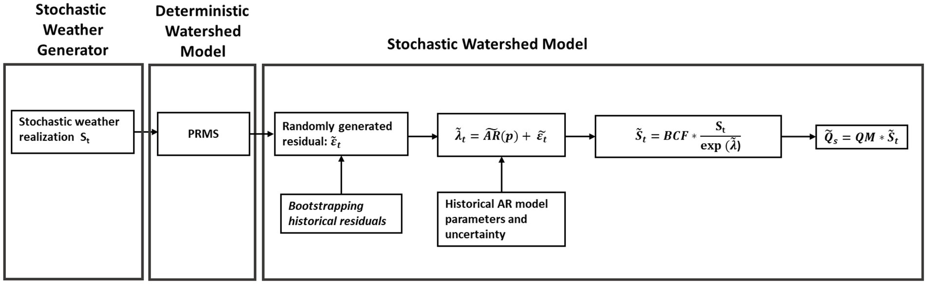
Figure 1. Integrated Stochastic Weather Generator (SWG)-Stochastic Watershed Model (SWM) framework to estimate hydrologic risk under climate change.
2.1 Study Basin
We demonstrate the proposed framework for the Squannacook River basin located in north-central Massachusetts and southern New Hampshire in the United States (see Figure 2). To demonstrate SWG-SWM framework’s generalizability, the SWG-SWM procedure was applied to a second basin (Shasta River basin, California, United States), with an alternative DWM, and different climate realizations. The results of that analysis are reported in the supplementary material. Previous studies suggest that the Northeast United States will experience the largest temperature increases in the contiguous United States (Hayhoe et al., 2018). Furthermore, a recent study in the state of Massachusetts projected an increase of more than 50% in the 100-year 24-h rainfall event for much of the state under both RCP4.5 and RCP8.5 emission scenarios (Siddique and Palmer, 2021). The Squannacook River basin was selected because it contains a 72-year continuous daily streamflow record, has relatively low regulation and hydrologic disturbance, and served as a pilot study for a previous SWM demonstration project (Shabestanipour et al., 2023).
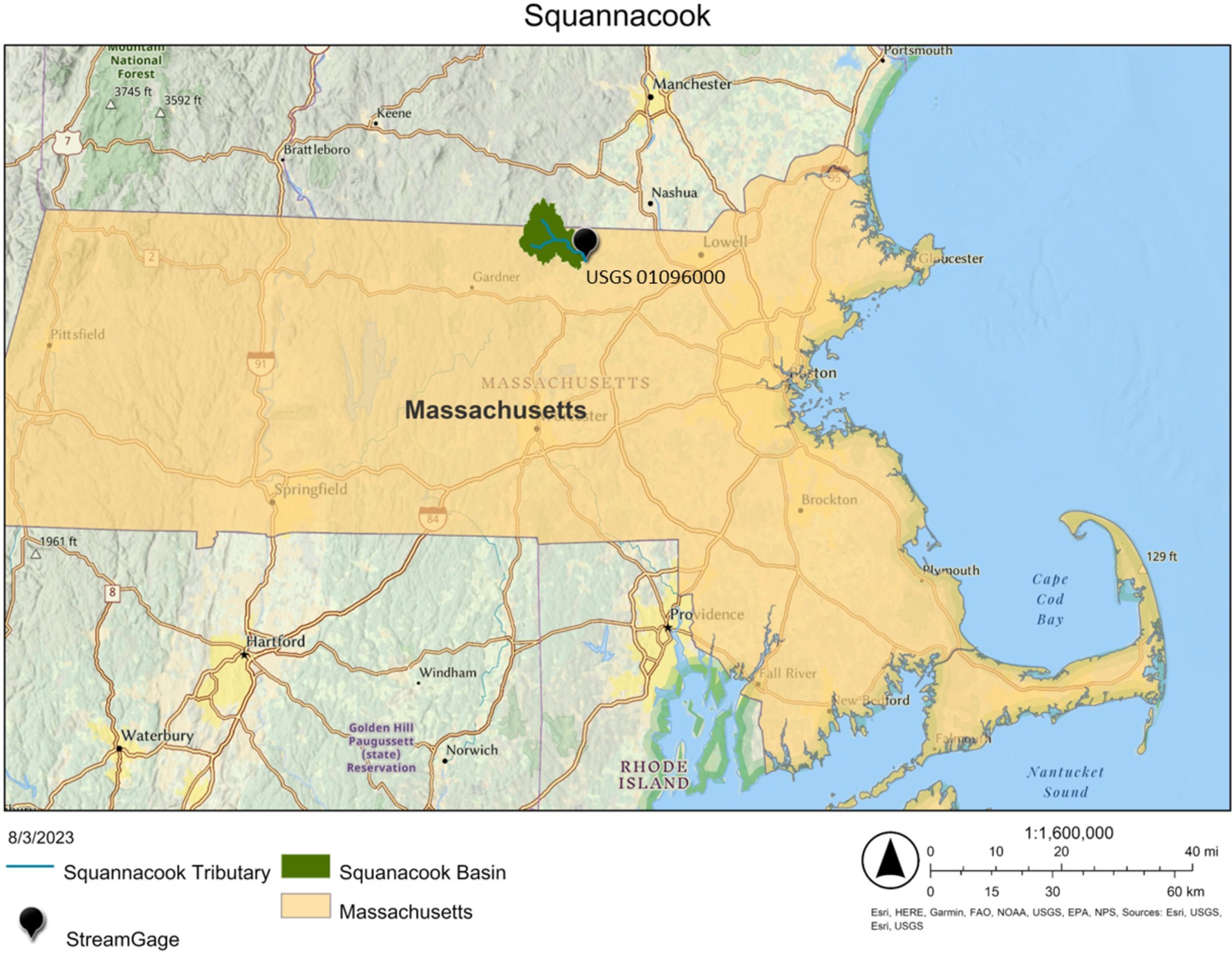
Figure 2. Location of the Squannacook River basin in Massachusetts, United States.
The Squannacook River drains southeasterly into the Nashua River, which in turn flows to the Merrimack River watershed and ultimately the Atlantic Ocean. The portion of the Squannacook River basin modeled in this study corresponds to the USGS streamgage 01096000, which has a drainage area of 173.8 km2. The watershed is primarily forested and contains more than 28 km2 of state and town forests. There are developed areas along key transportation corridors and in the center of Townsend, Massachusetts. Less than 8% of this basin area is impervious and it contains five dams. The basin topography ranges from a hilly upland plateau with maximum elevation of 450 m in the north and west to flat coastal plain in the south and east.
The climate in the Squannacook River basin is temperate, with mild summers and cold winters. The mean annual air temperature during 1981–2010 was about 46°F (7.78°C) with mean monthly air temperatures ranging from about 22°F (−5.5°C) in January to 69°F (20.5°C) in July (NOAA National Centers for Environmental Information, 2022). The mean annual precipitation is 48 inches (1,219 mm) (NOAA National Centers for Environmental Information, 2022), while the basin’s average annual potential evapotranspiration for the period of 1981–2010 is 23 inches (584 mm) (Northeast Regional Climate Center, 2024).
The DWM used in this pilot study is the USGS National Hydrologic Model Precipitation Runoff Modeling System (NHM-PRMS) version 5.1.0 (Markstrom et al., 2015; Regan et al., 2019). NHM-PRMS is a medium-complexity continuous watershed simulation model that is calibrated for the entire continental United States (Regan et al., 2019). The DAYMET climate dataset (Thornton et al., 2016) and available USGS streamflow records were used to configure and calibrate the NHM-PRMS. Calibration of NHM-PRMS is accomplished through a normalized squared error on streamflow along several calibration steps (e.g., high flows, low flows, monthly flows, and daily flows) for hydrologic response units. See Regan et al. (2019) for a full description of the calibration procedure. Minimal modification to the NHM-PRMS calibration was performed for this pilot study, including adjustment factors for minimum and maximum temperature, precipitation, precipitation-to-snow conversion, monthly air temperature coefficients used for potential evapotranspiration, and the groundwater discharge coefficient. The performance of the model in the Squannacook is adequate, with a Nash Sutcliffe efficiency of 0.64 and a log Nash Sutcliffe efficiency of 0.71. This is very similar to the average performance of PRMS across the United States (Farmer and Vogel, 2016).
2.2 Stochastic weather generator and climate scenarios
Stochastic weather generators provide a computationally efficient and complementary alternative to GCMs for hydrologic systems’ analysis under climate change. These models are structured based on historical meteorological records and are used to generate large ensembles of simulated daily weather records that are similar to but not bound by variability in past observations (Richardson, 1981; Wilks and Wilby, 1999; Fowler et al., 2007). For hydrologic impact assessment studies, weather generators must develop timeseries of multiple weather variables (e.g., precipitation and temperature) at multiple locations while maintaining the persistence and covariance structures associated with transient, multi-day storm events and over longer (seasonal-inter-annual) timescales. After a weather generator has been calibrated to historical data, model parameters can be adjusted to produce new realizations of weather, presenting changes in intensity and frequency of average and extreme precipitation, heatwaves, and cold spells (Wilks, 2002; Wilks, 2010; Wilks, 2012) The reasoning behind the specific methodological choices in the SWG used in this study are described in (Najibi and Steinschneider, 2023).
We adopt the SWG developed for the state of Massachusetts by Steinschneider and Najibi (2022a). This SWG is based on the model described in Steinschneider et al. (2019), Rahat et al. (2022), and Najibi et al. (2021). An advantage of the SWG over direct use of GCM projections, is the ability of the SWG to produce a larger number of climate change realizations at a spatial and temporal scale that is meaningful for hydrologic simulation, than what is typically available through direct use of downscaled GCMs. This weather generator is a semiparametric, multivariate, and multisite model that is designed to separately model dynamic and thermodynamic atmospheric mechanisms of climate variability and change through statistical abstractions of these processes. To capture atmospheric dynamics, the weather generator uses a non-homogenous Hidden Markov Model (NHMM) to identify and simulate sequences of weather regimes (WRs), which are recurring large-scale atmospheric flow patterns (e.g., upper-level, quasi-stationary blocks and troughs) that organize high-frequency weather systems (Robertson and Ghil, 1999; Robertson et al., 2015). Precipitation and both maximum and minimum temperature are simulated through bootstrapping from the historical record conditional on the simulated WRs. Noise is added to resampled heavy precipitation events to ensure that simulated extreme events can exceed those in the observations. To capture thermodynamic mechanisms of climate change, the weather generator post-processes simulated precipitation and temperature data to reflect patterns of warming and thermodynamic scaling of precipitation rates with that warming (i.e., precipitation intensification).
This model was developed for 20 separate river basins across the entire state of Massachusetts (at the 8-digit Hydrologic Unit Code: Huc8 level), using gridded (~6 km) daily precipitation and maximum and minimum temperature between January 1, 1950 and December 31, 2013 from the dataset developed by Livneh et al. (2015). For every HUC8 watershed, the model was used to simulate 100 ensemble members, each 64-years long (the length of the instrumental record), for temperature changes that range from 0°F to 8°F (0°C to 4.44°C) warming at 0.5°F (0.28°C) increments (17 warming scenarios altogether). This was the range of warming projected in the CMIP5 ensemble of future projections across the state of Massachusetts for all emission scenarios.
For each level of warming, extreme precipitation simulated by the model was scaled upwards using a quantile mapping approach. Specifically, the daily, non-zero precipitation distribution for each grid cell was stretched such that the 99.9th percentile was increased at the theoretical Clausius-Clapeyron (CC) scaling rate (~7% per °C warming), which is the rate at which the water holding capacity of the atmosphere increases with warming (Held and Soden, 2006). If all other factors controlling precipitation intensity remain unchanged, it is often assumed that extreme precipitation will scale with temperature at this same rate (Allen and Ingram, 2002; Allan and Soden, 2008). The reasoning is that under conditions that lead to extreme precipitation (i.e., near saturated atmospheric conditions; intense surface convergence and uplift), changes in atmospheric moisture content will translate directly to changes in precipitation amount. A separate analysis of extreme precipitation scaling across the Northeast US was used to support this choice (Najibi et al., 2022; Steinschneider and Najibi, 2022a). Mean precipitation was held at historical levels in these scenarios.
The climate change mechanisms that lead to hydrologic impact are categorized into thermodynamic or dynamic impacts of climate change. Thermodynamic impacts are directly related to the temperature change of the atmosphere. Thermodynamic modes include snow accumulation and melt, higher evapotranspiration, and more intense precipitation due to an increase in the moisture holding capacity of atmosphere. Dynamic atmospheric mechanisms refer to the frequency of weather regimes (i.e., shifts in atmospheric circulation) (Steinschneider and Najibi, 2022b), which are significantly more uncertain than thermodynamic change (Shepherd, 2014; Pfahl et al., 2017). The climate scenarios included in this analysis only reflect mechanisms of thermodynamic climate change, which are direct responses of the climate to warming and are often deemed some of the most credible projections of future climate (Pfahl et al., 2017). In this study we used the SWG simulations over the Squannacook River basin as the forcing to our hydrologic model, described next. Steinschneider and Najibi (2022a) found a substantial increase in the extreme rainfall intensity in the scenarios used for this study.
2.3 Stochastic watershed model
In this work we employ a SWM to translate scenarios of climate from the SWG into streamflow simulations. SWMs use a deterministic watershed model (DWM) to simulate the hydrologic response to climate, and then re-introduce errors back into the DWM prediction to address the bias in extreme flows (Vogel, 2017). In this work, we adopt the SWM developed in Shabestanipour et al. (2023), which was verified and validated for the Squannacook River basin. As described above, the USGS National Hydrologic Model Precipitation Runoff Modeling System (NHM-PRMS) (Regan et al., 2019) segment for the Squannacook River was used as the core DWM.
To add error back to the DWM predictions, the SWM in Shabestanipour et al. (2023) fits an autoregressive [AR(3)] model to the log-ratio (denoted 𝜆) of simulated and observed streamflow from the NHM-PRMS. Simulations of new log-ratios are then generated by first bootstrapping residuals from the fitted AR model, then using those resampled residuals in the AR model to re-introduce autocorrelation, and finally using those simulated log-ratios to adjust DWM simulated flows into a stochastic trace of simulated streamflow. There is also a separate bias correction factor (BCF) applied to address biases that can arise when operating on log-transformed flows. All equations for this model can be found in Figure 1.
We note that the PRMS model and the SWM in Shabestanipour et al. (2023) were both calibrated using observed meteorological data from the Daymet dataset (Thornton et al., 2016), but the SWG produces weather traces based on the meteorological data in Livneh et al. (2015). This change in input data introduces a bias to our simulated streamflows, which we address using a quantile mapping bias correction calibrated over the historical period (see Supporting Information; Teegavarapu et al., 2019).
Ultimately, we force the DWM with the 17 different warming scenarios from the SWG, each containing 100 ensemble members, for a total of 1,700 separate time series of deterministic streamflow predictions. We then used the SWM to simulate 10,000 stochastic streamflow traces for each of these 1,700 realizations, producing a super ensemble of 17,000,000 streamflow traces. Here, each of the 17 warming scenarios (which capture future climate change uncertainty) have 1,000,000 hydrologic simulations that capture both natural climate variability and hydrologic model uncertainty.
2.4 Risk-of-failure design criterion
By integrating the SWG and SWM above, we can simulate a super ensemble of streamflow traces associated with 17 separate levels of future warming. However, these traces (which are each 64 years long) reflect a different step change in temperature rather than gradual, transient scenarios of warming. Therefore, the ensemble of 1,000,000 streamflow traces associated with each level of warming can be used to calculate the stationary risk of infrastructure failure for a particular level of warming, but they cannot be directly used to calculate the risk of failure over a T-year planning horizon during which temperatures gradually warm.
We address this challenge by first calculating the stationary risk of failure for each warming scenario generated by the SWG-SWM ensemble, and then integrate this risk of failure over transient pathways of warming projected by GCMs. To demonstrate this approach, let A be a particular flood magnitude of concern (e.g., the flood level that would exceed the capacity of a planned infrastructure project). We then define the probability that the flood magnitude A will not be exceeded for a particular warming scenario W ∊ [0°F (0°C), 8°F (4.44°C)] as:
There are two considerations in the formulation above that require discussion. First, the transient warming for each year t in the planning horizon needs to be specified. For illustration, we do this using a transient projection of temperature from the GFDL-ESM2G GCM forced with two separate emission scenarios (RCP 4.5 and RCP8.5) and downscaled using the Multivariate Adaptive Constructed Analogs approach (MACA; Abatzoglou and Brown, 2012). For each RCP, we compare the historical temperatures from this model to the predicted future temperatures and set to the warming level at the end of each decade out to 2,100. That is, annual values of increase upwards once every decade over a planning horizon of T = 77 years (assuming a starting year of 2025). In this step, we used the decadal time steps in order to both decrease the noise from interannual variability and the necessary computational power.
Second, the probability P(A|W) is only available for the discrete levels of warming generated by the SWG (0°F to 8°F at 0.5°F increments), but can reflect any level of warming occurring at year t in the planning horizon. Therefore, if is between one of the increments of warming produced by the SWG, the probability is estimated by linearly interpolating between the probabilities P(A|W) for SWG-informed warming levels that are directly above and below .
3 Results and discussion
The integrated SWG-SWM framework described in Section 2 allows planners and engineers to track the impacts of climate change on the distribution of key design statistics for varying levels of warming or over climate change scenarios, or alternatively to evaluate the risk of a given flow being exceeded over the intended design life of a project. We address each of these two cases in turn for the Squannacook River in Sections 3.1 and 3.2 below.
3.1 Non-stationary design events
Figure 3 compares the distribution of several common drought and flood design statistics under vary levels of warming to the observed values over the historical period (1950–2013). Observed values are derived by fitting a log-Pearson Type III distribution to the annual maximum or 7-day low flow series (Chowdhury and Stedinger, 1991). For each of the flood statistics, the SWG-SWM simulations for 0°F /0C warming closely match the observational record, producing similar median and 90% confidence intervals. This indicates that the SWG-SWM framework can replicate flood characteristics under historical conditions and suggests the model should provide reasonable projections of flood characteristics under warming conditions. The SWG-SWM framework struggles to capture the uncertainty in the estimate of the 7Q10 (minimum annual 7-day average flow with 10-year recurrence interval) from the observational record, which is likely due in part to the underlaying hydrologic model’s poor performance in simulating low flows in the Squannacook (Shabestanipour et al., 2023). Despite this, the SWM-SWG median 7Q10 is close to the observed 7Q10 and is well within the 90% confidence interval (see 0°C scenario width of calculated 7Q10s in Figure 3A).
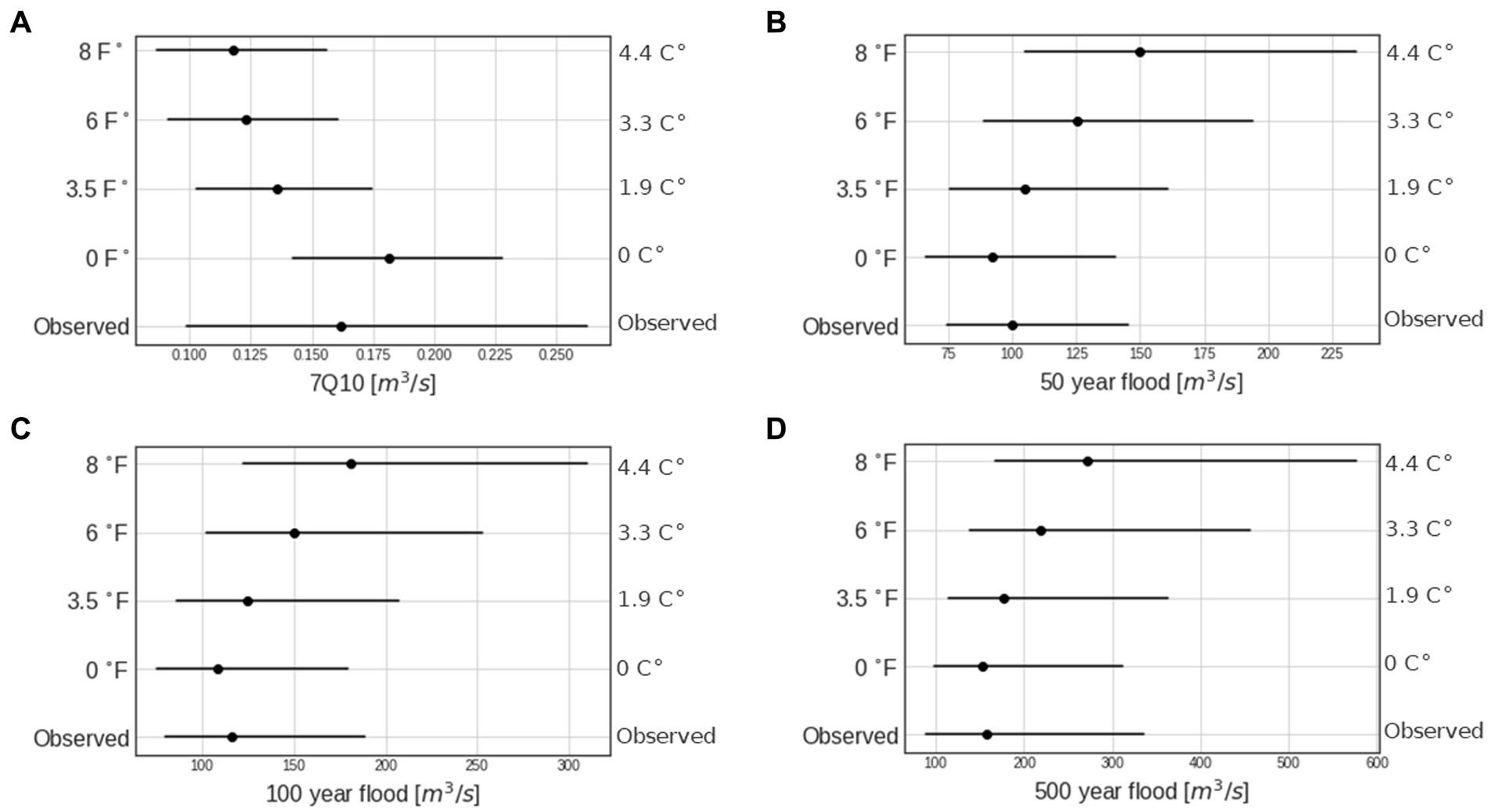
Figure 3. Impact of fixed warming levels on the distribution of the (A) 7Q10, (B) 50-year flood, (C) 100-year flood, and (D) 500-year flood.
The SWG-SWM framework projects that both droughts and floods will become more extreme as temperatures increase in the Squannacook. For example, under 4°F (2.22°C) warming the SWG-SWM projects an increase in the median100-year flood of 19% over 0°F (0°C) conditions, and an increase of 68% under 8°F (4.44°C) warming. For a fixed AEP flood, the marginal flood magnification with respect to an increase in warming also increases, so flood magnification is a non-linear function of warming for the Squannacook. For a fixed warming level, the flood magnification also increases with return period. For example, under 8°F (4.44°C), the SWG-SWM projects an increase of 63, 68, and 78% for the 50-, 100-, and 500-year floods, respectively. There is significant uncertainty in both the observed and projected flood magnitudes, as reflected in the wide 90% confidence intervals in Figure 3. The projected median 100- and 500-year floods are within the 90% confidence interval of the observed historical record, as estimating such extreme flood quantiles from a limited historical record includes significant uncertainty. The projected distributions of extreme floods are positively skewed, with upper tails that extend to extreme flood magnitudes, and this asymmetry grows with warming conditions.
While the fixed warming levels in Figure 3 are useful to track the basin response to warming, climate change is expected to evolve through the course of the 21st century and most planning exercises use climate scenarios, such as the representative concentration pathways (RCPs) (Van Vuuren et al., 2011). Figure 4 plots the evolution of the median daily flow, the 100-year flood, and the 500-year flood for RCP4.5 and RCP8.5 by decade through 2,100, by mapping the GCM-projected temperature change under each emission scenario and for each target year to a SWG-SWM warming scenario. The no-warming scenario is also shown as a baseline. The SWG-SWM framework projects a decline in the median daily flow through 2,100 under both climate scenarios: a 21% decline for RCP4.5 and a 33% decline for RCP8.5. Despite this, extreme flood magnitudes are projected to increase under both RCPs. Under RCP4.5 extreme flood magnification is modest, with a median flood magnification of 15% for the 100-year flood and 17% for the 500-year flood by 2,100. Even by the end of the century, under RCP4.5 the median 100- and 500-year flood magnitudes are well within the 90% confidence interval for the no-warming case, reflecting both the uncertainty in extreme flood estimation and the limited impact of modest warming on extreme flood quantiles (see also Figure 3). RCP8.5 sees more substantial shifts in the distribution of extreme floods by 2,100, with a 67 and 77% increase in the 100- and 500-year median floods, respectively. Flood magnification quickens after 2050, when RCP8.5 projects a more rapid rise in global warming levels. By 2,100 under RCP8.5, the SWG-SWM framework projects that the 100-year flood magnitude will exceed the estimated 500-year flood over the historical period. This behavior is due to the fact that global temperature change of the RCP8.5 scenario starts to vary significantly from the RCP4.5 scenario after 2050 (Ansuategi et al., 2015).
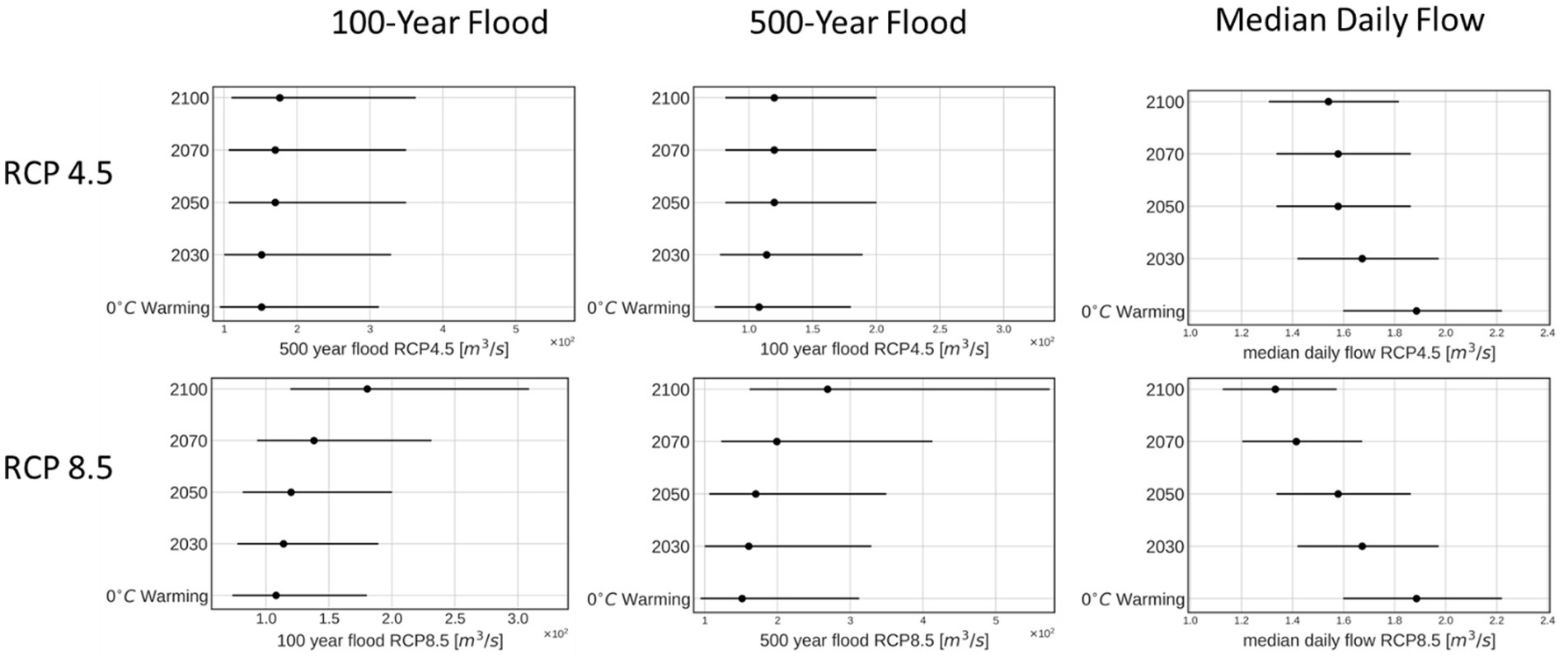
Figure 4. Design floods and median daily flows by decade under RCP4.5 and RCP8.5 and under 0°F/°C warming.
Previous studies in the region project approximately a 30% increase in the 100-year flood in western and central Massachusetts under RCP8.5 (Siddique et al., 2020; Siddique and Palmer, 2021), which is less extreme than our results. Both our study and previous studies suggest greater increase around the end of the century. Our results for RCP4.5 are in general agreement with previous work, which estimate an approximate 15% increase of the 100-year flood under this warming trajectory (Siddique and Palmer, 2021).
3.2 Risk of failure
Figure 4 provides a useful demonstration of shifting extremes in a non-stationary world by tracking changes in common design statistics over time for different climate scenarios. Figure 4 also highlights the deficiency of the “return period” or the AEP as a concept for communicating risk under non-stationarity. The median 100-year flood can be expected to change over the design life of infrastructure built today due to climate change (Milly et al., 2002). In the case of the Squannacook, the 100-year flood is expected to get larger over time. Planning for the 100-year flood today risks under-design, whereas planning for the 100-year flood at the end of the planning horizon risks over-design. Non-stationary return periods have been proposed (Olsen et al., 1998; Salas and Obeysekera, 2014), but their meaning can be difficult to interpret. A more natural design criteria is risk (or conversely, reliability), whose interpretation is the same under stationary or non-stationary conditions (Read and Vogel, 2015).
Figure 5 reports the relationship between risk and various fixed return period floods under a range of warming conditions, for a 50-year design life. Figure 5A illustrates how the risk of the no-warming 50-year, 100-year, and 500-year floods change for the Squannacook as temperatures increase. As expected from Equation 2, the risk of the no-warming 50-, 100-, and 500-year events being exceeded in a 50-year design life under the no-warming case are about 60, 40, and 10%, respectively. As temperatures warm in the Squannacook, the risk of each design event being exceeded increases substantially, with 4.5°F of warming the risk of the no-warming 100-year event exceeding the theoretical risk of the 50-year flood in stationary conditions. The relationship between risk and warming is nonlinear and varies by return period. At low warming levels, the risk of the 50-year flood increases more rapidly with temperature in absolute terms than risk of the 500-year event. However, the opposite is true at high warming levels, with the 500-year flood’s risk increasing with temperature faster than the 50-year flood. Figure 5B shows the percent change in risk for the three design events under varying degrees of warming. For a fixed level of warming, the relative increase in risk grows with return period. For example, under 6°F of warming, the risk of the 50-year flood has increased 58% while the 500-year flood risk has increased 186%. As temperatures increase, the relative increase in the risk of the 500-year flood grows rapidly, while the relative increase in the risk of the 50-year event stagnates as it approaches 100% risk in absolute terms (e.g., near certainty that it will be exceeded over the 50-year design life).
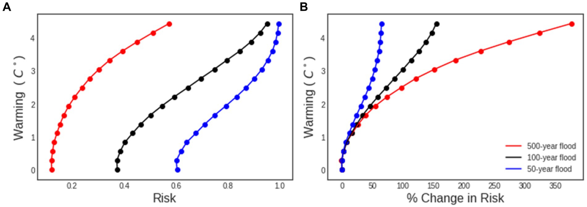
Figure 5. (A) The impact of warming on the risk of no-warming design events over a 50-year design life. (B) Percent change in risk of no-warming design events over a 50-year design life.
Figure 6 reports the accumulated risk of various design floods (computed under no warming), being exceeded over time under three future climate scenarios: no-warming, RCP4.5, and RCP8.5. Risk increases over time, as each year there is a chance the specified design flow will be exceeded. The risk increases faster for less-extreme floods (e.g., 50-year flood), as each year there is a higher probability that flow level will be exceeded. Risk also grows more quickly for the two warming scenarios than for the no-warming case, because the SWG-SWM projects that increasing temperatures will increase extreme floods. The difference in risk between RCP4.5 and the no-warming case is notable, given the SWG-SWM framework projects only modest increases in extreme floods under RCP4.5 (see Figure 4). This highlights that even small increases in annual flood risk compound over time to yield substantial differences in risk over a long planning horizon. There is very little difference between RCP4.5 and RCP8.5 through 2050, because those two climate scenarios follow similar warming trajectories until mid-century. After 2050, risk accumulates quicker for RCP8.5 than RCP4.5, as the SWM-SWG projects that floods will become more extreme under RCP8.5 than RCP4.5. Figure 6 suggests that the choice of climate scenario (RCP4.5 vs. RCP8.5) does not meaningfully impact flood risk if the planning horizon terminates around 2050, but that after 2050 the choice of climate scenario can impact the projected flood risk.

Figure 6. Accumulated risk of no-warming design events over the 21st century for the RCP4.5, RCP8.5, and no-warming scenarios.
To further explore generalizability of this framework we implemented the SWG-SWM integration process for the Shasta River basin in California, United States. We have included the results of secondary basin’s analysis in the supplementary material. Implementation of the framework on a second basin supports the applicability of this method on basins with different hydrologic characteristics.
3.3 Risk-based decision making using the SWM-SWG framework
To demonstrate the application of the SWG-SWM framework for risk-based decision making, we consider the design of culvert with a 50-year design life being constructed in 2025. In Massachusetts, the recommended design flow for a culvert is the 100-year flood (Massachusetts Department of Transportation, 2020). Under stationary conditions, this implies a 39.5% risk over the design life. When designing a culvert in non-stationary conditions, the planner has at least three choices in selecting a design flow: (1) design to the current 100-year flood (here represented by the no-warming case), (2) design to the 100-year flood at the end of the design life under a climate scenario, or (3) design to a flow that matches the desired risk implied by current design standards (i.e., 39.5%). Figure 7 plots the design-life risk associated with each of those options for RCP4.5 and RCP8.5 versus the design flow. For choice 1 and 2 the associated risk of the design flow is calculated by Equation (2) and the third design flow was found by a grid search for the associated risks of flows in between the two initial flows. Here the design flow can be considered a proxy for cost, albeit an approximate and non-linear one. Each line represents an alternative climate scenario, which is uncertain and represents a design choice. An ideal solution (given a climate scenario) would be one in the lower left of Figure 7: a low-risk solution with a small design flow and consequently a smaller cost. Unfortunately, the ideal is not possible, and a compromise must be selected.
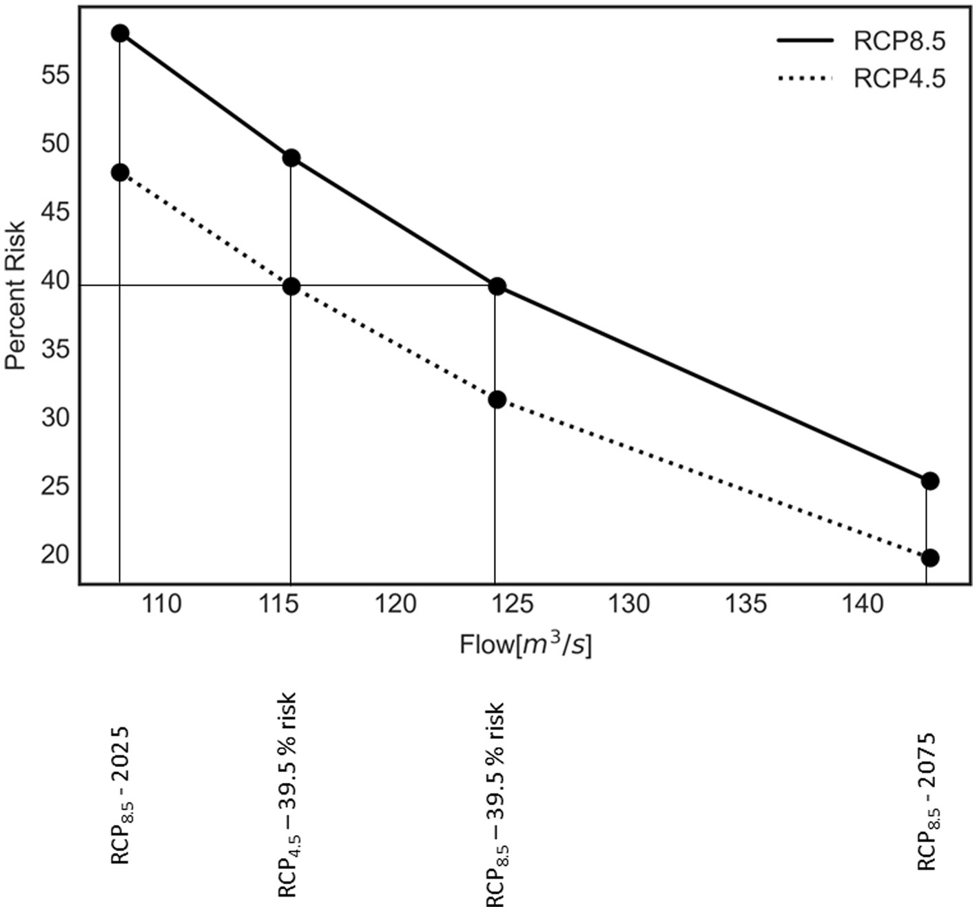
Figure 7. Risk over a 50-year design life under RCP4.5 and RCP8.5 for alternative design flows.
The current (no-warming) 100-year flood is roughly 3,800 cfs (107 ) and corresponds to a life-time risk of about 40% under stationary conditions. However, the risk of the current design flow is substantially higher under climate scenarios: rising to 48% under RCP4.5 and 58% under RCP8.5. Thus, utilizing the current 100-year flood results in under-design and unacceptable levels of risk in the Squannacook under climate change, according to design standards. Instead, planners may opt to design for the 100-year flood at the end of the design life, in this case 2075. As the SWG-SWM framework projects increasing flood magnitudes through the course of the 21st century, this may be perceived as a sensible, conservative choice. However, this will result in significantly lower risk than desired in the design codes. Under RCP8.5, the SWG-SWM projects the 2075 100-year flood to be about 5,000 cfs (141.5 ), corresponding to a risk of 25.3%. On its face, a lower risk seems desirable, but it also represents a significant over design: a flow of about 4,400 cfs (124.6 ) achieves the desired 39.5% risk under RCP8.5. If the actual warming is less extreme than RCP8.5, which is likely (Hausfather and Peters, 2020; Hausfather et al., 2022; Voosen, 2022), then the overdesign and consequently the regret will be even more extreme. A thorough economic analysis of the costs of over- vs. under-design is beyond the scope of this simple example, but if the design standards reflect societal risk-tolerance, then selecting the 100-year flood at the end of the design life reflects over design, and a potential inefficient use of resources that might be spent elsewhere in support of other societal objectives.
As shown in Figure 4, RCP4.5 projects more moderate changes to extreme floods over the 21st century than RCP8.5. The SWG-SWM projects the 100-year flood to be about 4,200 cfs (118.9 ) in 2075 under RCP4.5, while the flow required to achieve the desired 39.5% is about 4,100 cfs (116 ). Thus, designing for the 100-year flood in 2075 under RCP4.5 represents only a slight overdesign, with an actual risk of 35.7%. Of course, the future will not follow exactly the scenario selected for planning, so it is instructive to consider the loss or gain of risk if an alternative climate scenario occurs than the one planned for. For example, if the 2075 100-year flood from RCP8.5 is used for planning, but RCP4.5 actually occurs, the associate risk is 19.7% compared to the desired 39.5% and the infrastructure would be designed for a flow that is nearly 1,000 cfs (28.3 ) larger than required to achieve the desired risk. The regret of overdesign could be quantified monetarily in a more applied problem. In contrast, if the design flow is selected to achieve 39.5% risk under RCP8.5, and RCP4.5 actually occurs, the associated risk would be 31.3% rather than the desired 39.5% and the infrastructure would be designed to a flow only about 300 cfs ( ) larger than required. Thus, if planning for RCP8.5, adopting a risk framing rather than the end-of-horizon 100-year flood reduces the regret of overdesign substantially. This result arises in part because RCP4.5 and RCP8.5 follow similar trajectories through 2050, so the flow associated with a life-time risk of 39.5% is quite similar, even if their 2075 100-year floods are quite different.
Figure 8 plots risk vs. flow for two planning horizons (50 and 70 years starting in 2025) and two climate scenarios (RCP4.5 and RCP8.5). This diagram can be used by practitioners to identify a design flow associated with a desired risk, planning horizon, and climate scenario, or alternatively a practitioner could identify the risk associated with a given flow, planning horizon, and climate scenario. The 50-year planning horizon risk profiles are similar between RCP4.5 and RCP8.5, largely because their warming trajectories are quite close into the middle of the 21st century. Because both RCP4.5 and RCP8.5 project rising temperatures through the end of the 21st century, the SWM-SWM projects increasing flood magnitudes through 2,100 (see Figure 4). Thus, the longer the planning horizon stretches into the future, the more the risk-profile shifts to the right (greater flows associated with a fixed risk). The relative shift in the risk profile between the 50- and 70-year planning horizon is greater for RCP8.5 than RCP4.5, reflecting the greater projected late-century warming under RCP8.5. Using the simulation ensemble from the SWG-SWM framework, Figure 8 can be expanded to include alternative planning horizons or new climate scenarios.
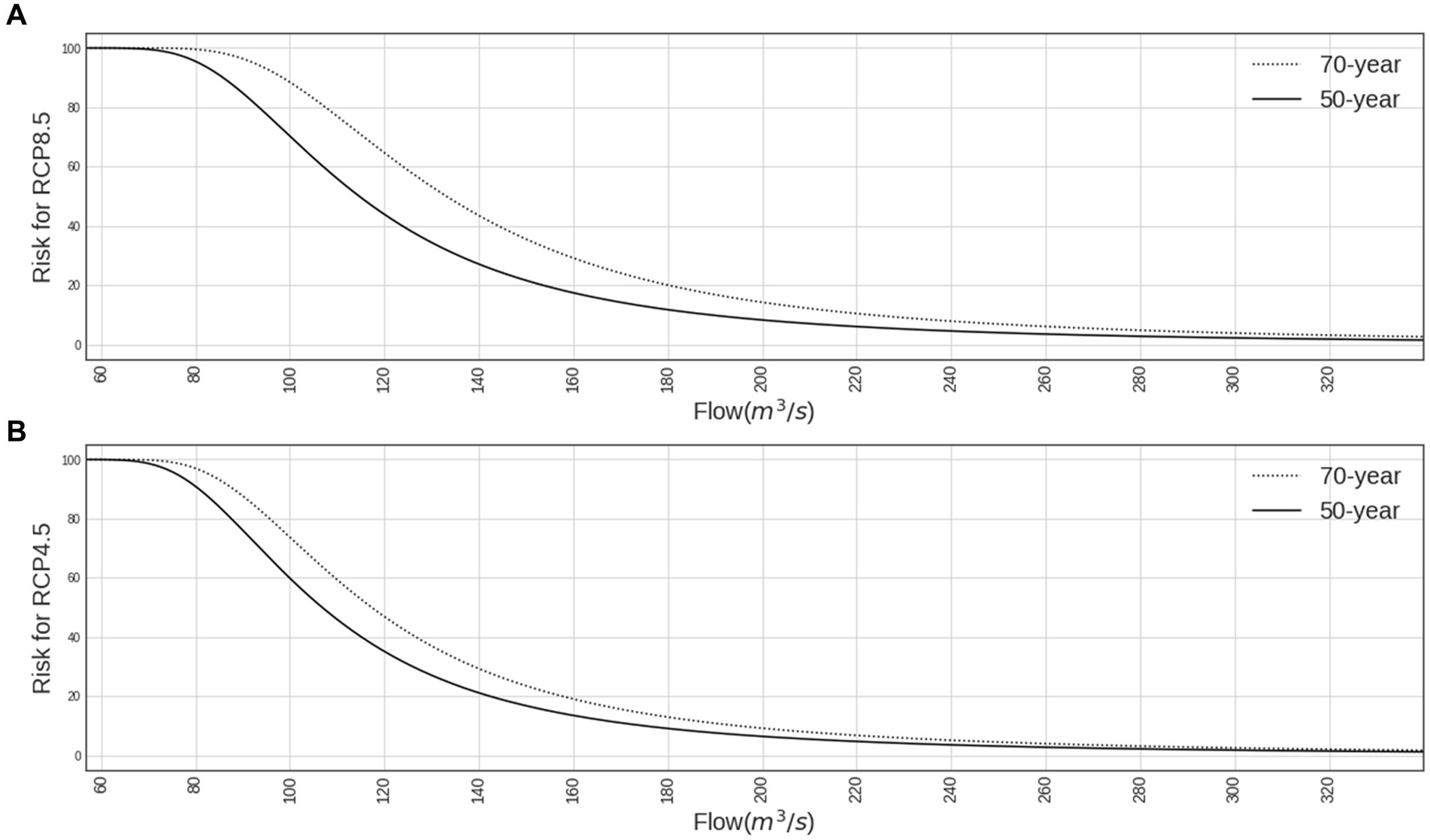
Figure 8. Risk versus flood magnitude for infrastructure built in 2025 with either a 50-year or 70-year design life, under (A) RCP8.5 and (B) RCP4.5.
4 Conclusion
Climate change is expected to alter the distribution and arrival of hydrologic extremes, and this presents a significant challenge to long-term water resources planning and management. Mapping the hydrologic response to changing climate drivers is challenging, in part because of a mismatch in the scale and focus of common climate and hydrologic models with the needs of local planners. More fundamentally, non-stationarity renders the interpretation of common design statistics, like the 100-year flood, technically ambiguous and of dubious practical value. To address both issues, this work presents a computational framework for risk-based decision making at the basin-scale, composed of a Stochastic Weather Generator (SWG) and a Stochastic Watershed Model (SWM). The SWG is used to produce many synthetic weather sequences reflecting different levels of warming and associated intensification of extreme precipitation, while using abstractions of dynamic atmospheric mechanisms to capture key signals of natural climate variability. The SWM captures the hydrologic response to changing climate forcing, correcting bias in the deterministic hydrologic models’ representation of extreme flows by properly capturing the variance of daily streamflow. The integrated SWG-SWM framework is applied to the Squannacook River basin in Massachusetts to illustrate the impact of climate change on the distribution of hydrologic extremes and use of risk in hydrologic design.
For the Squannacook, the SWG-SWM framework projects that warming temperatures will produce more extreme floods and low flow events. The increase in flood magnitude is non-linear with respect to warming: the marginal increase in flood magnitude with respect to an increase in temperature increases with the warming level. The increase in flood magnitude with warming is also greater for more extreme floods: the relative increase of the 500-year flood is greater than the relative increase of the 100-year flood for a fixed warming level. Still, the uncertainty in extreme floods under no warming is sufficiently large to encompass median estimates of extreme flooding under a high degree of warming.
A similar non-linear pattern is seen for the risk of failure of a specified flood magnitude over a given planning horizon. For smaller flood magnitudes, the risk saturates toward unity for moderate horizons (e.g., T = 50 years) as it becomes near certain that those events will be exceeded, while for larger floods the risk grows exponentially (on a percentage basis). Importantly, the accumulated risk associated with flooding is similar between moderate and high emission scenarios during the first half of the 21st century because the two scenarios follow similar warming trajectories until around 2050. This result has large implications for reducing regret in hydrologic design. Our results show that basing hydrologic designs on return period estimates at either the beginning or the end of a planning horizon can lead to large regret (under- or over-design), especially if a different climate future occurs than the one used to guide design. This regret can be reduced if design is based on a risk framing, largely because different emission scenarios (RCP4.5 and RCP8.5) follow similar warming trajectories through mid-century, so the flow associated with a given life-time risk of failure is more similar than the end-of-horizon return period events.
While the SWG-SWM framework to support risk-based hydrologic design proposed in this work shows promise, several limitations of the method require discussion. First, the SWG is designed to propagate key signals of climate change into large ensembles of future weather for risk analysis, but the model is not governed by the physical laws of the climate system and therefore may produce weather ensembles that are not physically plausible, especially for extreme climate change scenarios. In addition, the SWG was only used in this study to create scenarios of warming and extreme precipitation intensification, without consideration of other signals of potential climate change (e.g., shifts in seasonality, changes in mean precipitation, etc.). A more in-depth analysis could use the SWG to expand the set of scenarios tested, or alternatively, multiple single model initial condition large ensembles (SMILES, Lehner et al., 2020) could be used as the basis for the weather ensembles in our risk-based framework. In either case, multiple signals of future climate change beyond just warming could interact to influence hydrologic risk-of-failure, and these effects should be disentangled (e.g., using variance decomposition); (Steinschneider et al., 2023) to understand the relative importance of different climate change signals on risk. This effort will be the focus of future work.
A second important limitation of this work is the assumption in the SWM that the error structure observed historically can be used to propagate hydrologic model uncertainty under new climate conditions. Climate change will alter the frequency, timing, and intensity of hydrologic model states, activate model components in configurations not seen in the historical record, and change the way meteorological forcing is converted to streamflow. These changes could alter the structure and distribution of hydrologic model errors, although it is difficult to anticipate these changes because no future observations are available against which to estimate shifts in the error distribution. One promising approach to address this challenge is to link the error distribution in SWMs to hydrologic model state variables, so that changes in the frequency of different states under climate change trigger an associate shift in the error distribution. This is an active topic of ongoing research. Another limitation of this work is we do not consider any land-use change for future scenarios. Future work for long-term decision making should consider various combinations of land-use change scenarios and warming scenarios.
More broadly, we argue that there is a need for practitioners in hydrologic engineering to move away from conventional approaches to design such as return period-based design event estimation. These techniques, while suitable in the past, are no longer justified given the accelerating rate at which the risk of extreme events is changing, and the propensity of these methods to lead to the future under- or over-design of infrastructure. Instead, we argue that risk-based approaches like the one forwarded in this work and advocated elsewhere (Read and Vogel, 2015) provides an intuitive approach that is well-suited for a future in which risk is highly uncertain and dynamic. We recognize that the legacy of return period event-based design is entrenched in the current state of practice for hydrologic engineering. Therefore, as new methodologies emerge to support risk-based approaches, we argue that equal or more effort is needed to advocate for their use in practice, including the introduction of such alternative approaches in undergraduate and graduate school curricula.
Data availability statement
The datasets presented in this study can be found in online repositories. The names of the repository/repositories and accession number(s) can be found at: https://doi.org/10.5281/zenodo.8393390.
Author contributions
GS: Conceptualization, Formal analysis, Methodology, Writing – original draft, Data curation, Investigation, Software, Validation, Visualization. ZB: Data curation, Formal analysis, Writing – review & editing. BM: Formal analysis, Writing – review & editing, Investigation, Data curation, Software, Visualization. AB: Formal analysis, Writing – review & editing, Investigation, Software, Visualization. SS: Conceptualization, Formal analysis, Funding acquisition, Investigation, Methodology, Supervision, Validation, Writing – original draft, Writing – review & editing. JL: Conceptualization, Formal analysis, Funding acquisition, Methodology, Resources, Supervision, Writing – original draft, Writing – review & editing.
Funding
The author(s) declare financial support was received for the research, authorship, and/or publication of this article. This work was supported by the Massachusetts Executive Office of Energy and Environmental Affairs.
Conflict of interest
The authors declare that the research was conducted in the absence of any commercial or financial relationships that could be construed as a potential conflict of interest.
Publisher’s note
All claims expressed in this article are solely those of the authors and do not necessarily represent those of their affiliated organizations, or those of the publisher, the editors and the reviewers. Any product that may be evaluated in this article, or claim that may be made by its manufacturer, is not guaranteed or endorsed by the publisher.
Supplementary material
The Supplementary material for this article can be found online at: https://www.frontiersin.org/articles/10.3389/frwa.2024.1310590/full#supplementary-material
References
Abatzoglou, J. T., and Brown, T. J. (2012). A comparison of statistical Downscaling methods suited for Wildfire Applications: statistical downscaling for wildfire applications. Int. J. Climatol. 32, 772–780. doi: 10.1002/joc.2312
Allan, R. P., and Soden, B. J. (2008). Atmospheric warming and the amplification of precipitation extremes. Science 321, 1481–1484. doi: 10.1126/science.1160787
Allen, M. R., and Ingram, W. J. (2002). Constraints on future changes in climate and the hydrologic cycle. Nature 419, 224–232. doi: 10.1038/nature01092
Ansuategi, A., Delgado, J., and Galarraga, I. (2015). Green energy and efficiency: an economic perspective. Cham: Springer International Publishing.
Balting, D. F., AghaKouchak, A., Lohmann, G., and Ionita, M. (2021). Northern hemisphere drought risk in a warming climate. NPJ Climate Atmospheric Sci. 4:61. doi: 10.1038/s41612-021-00218-2
Chowdhury, J. U., and Stedinger, J. R. (1991). Confidence interval for design floods with estimated skew coefficient. J. Hydraul. Eng. 117, 811–831. doi: 10.1061/(ASCE)0733-9429(1991)117:7(811)
Cooley, D. (2012). “Return periods and return levels under climate change” in Extremes in a changing climate: Detection, analysis and uncertainty. (Dordrecht, Netherlands: Springer), 97–114.
Douglas, E. M., Vogel, R. M., and Kroll, C. N. (2002). Impact of streamflow persistence on hydrologic design. J. Hydrol. Eng. 7, 220–227. doi: 10.1061/(ASCE)1084-0699(2002)7:3(220)
Farmer, W. H., and Vogel, R. M. (2016). On the deterministic and stochastic use of hydrologic models. Water Resour. Res. 52, 5619–5633. doi: 10.1002/2016WR019129
Fernández, B., and Salas, J. D. (1999). Return period and risk of hydrologic events. I: mathematical formulation. J. Hydrol. Eng. 4, 297–307. doi: 10.1061/(ASCE)1084-0699(1999)4:4(297)
Fowler, H. J., Blenkinsop, S., and Tebaldi, C. (2007). Linking climate change modelling to impacts studies: recent advances in Downscaling techniques for hydrological modelling. Int. J. Climatol. 27, 1547–1578. doi: 10.1002/joc.1556
Gumbel, E. J. (1941). The return period of flood flows. Ann. Math. Stat. 12, 163–190. doi: 10.1214/aoms/1177731747
Haghighatafshar, S., Becker, P., Moddemeyer, S., Persson, A., Sörensen, J., Aspegren, H., et al. (2020). Paradigm shift in engineering of pluvial floods: from historical recurrence intervals to risk-based Design for an Uncertain Future. Sustain. Cities Soc. 61:102317. doi: 10.1016/j.scs.2020.102317
Hausfather, Z., Marvel, K., Schmidt, G. A., Nielsen-Gammon, J. W., and Zelinka, M. (2022). Climate simulations: recognize the ‘hot model’ problem. Nature 605, 26–29. doi: 10.1038/d41586-022-01192-2
Hausfather, Z., and Peters, G. P. (2020). RCP8.5 is a problematic scenario for near-term emissions. Proc. Natl. Acad. Sci. 117, 27791–27792. doi: 10.1073/pnas.2017124117
Hawcroft, M., Walsh, E., Hodges, K., and Zappa, G. (2018). Significantly increased extreme precipitation expected in Europe and North America from extratropical cyclones. Environ. Res. Lett. 13:124006. doi: 10.1088/1748-9326/aaed59
Hayhoe, K., Wuebbles, D. J., Easterling, D. R., Fahey, D. W., Doherty, S., et al. (2018). Chapter 2: our changing climate. impacts, risks, and adaptation in the United States: The fourth national climate assessment, volume II. U.S. Global Change Research Program.
Held, I. M., and Soden, B. J. (2006). Robust responses of the hydrological cycle to global warming. J. Clim. 19, 5686–5699. doi: 10.1175/JCLI3990.1
Intergovernmental Panel On Climate Change (Ipcc) . (2023). Climate change 2022 – impacts, adaptation and vulnerability: working group II contribution to the sixth assessment report of the intergovernmental panel on climate change (1st Edn.). Cambridge: Cambridge University Press.
Kendon, E. J., Ban, N., Roberts, N. M., Fowler, H. J., Roberts, M. J., Chan, S. C., et al. (2017). Do convection-permitting regional climate models improve projections of future precipitation change? Bull. Am. Meteorol. Soc. 98, 79–93. doi: 10.1175/BAMS-D-15-0004.1
Koutsoyiannis, D., and Montanari, A. (2022). Bluecat: A local uncertainty estimator for deterministic simulations and predictions. Water Resour. Res. 58, 1–20. doi: 10.1029/2021WR031215
Kyselý, J., Rulfová, Z., Farda, A., and Hanel, M. (2016). Convective and Stratiform precipitation characteristics in an Ensemble of Regional Climate Model Simulations. Clim. Dyn. 46, 227–243. doi: 10.1007/s00382-015-2580-7
Lehner, F., Deser, C., Maher, N., Marotzke, J., Fischer, E. M., Brunner, L., et al. (2020). Partitioning climate projection uncertainty with multiple large ensembles and CMIP5/6. Earth Syst. Dynam. 11, 491–508. doi: 10.5194/esd-11-491-2020
Livneh, B., Bohn, T., and Pierce, D. (2015). A spatially comprehensive, hydrometeorological data set for Mexico, the U.S., and Southern Canada 1950–2013. Sci Data. 2, 150042. doi: 10.1038/sdata.2015.42
Lu, J., Ruby Leung, L., Yang, Q., Chen, G., Collins, W. D., Fuyu Li, Z., et al. (2014). The robust dynamical contribution to precipitation extremes in idealized warming simulations across model resolutions: Lu et al.: dynamic effect on precipitation extreme. Geophys. Res. Lett. 41, 2971–2978. doi: 10.1002/2014GL059532
Maher, N., Milinski, S., Suarez-Gutierrez, L., Botzet, M., Dobrynin, M., Kornblueh, L., et al. (2019). The max Planck institute grand ensemble: enabling the exploration of climate system variability. J. Adv. Model. Earth Syst. 11, 2050–2069. doi: 10.1029/2019MS001639
Markstrom, S.L., Regan, R.S., Hay, L.E., Viger, R.J., Richard, M.T, Webb, Robert A, et al., (2015). PRMS-IV, the precipitation-runoff modeling system, version 4 (No. 6-B7). US Geological Survey.
Massachusetts Department of Transportation . (2020). “LRFD bridge manual -bridge site exploration.” Massachusetts Department of Transportation. Available at: https://www.mass.gov/info-details/part-i-design-guidelines.
Milly, P. C. D., Wetherald, R. T., Dunne, K. A., and Delworth, T. L. (2002). Increasing risk of great floods in a changing climate. Nature 415, 514–517. doi: 10.1038/415514a
Moges, E., Demissie, Y., Larsen, L., and Yassin, F. (2020). Review: sources of hydrological model uncertainties and advances in their analysis. Water. 13:28.
Muñoz, Á. G., Yang, X., Vecchi, G. A., Robertson, A. W., and Cooke, W. F. (2017). A weather-type-based cross-time-scale diagnostic framework for coupled circulation models. J. Clim. 30, 8951–8972. doi: 10.1175/JCLI-D-17-0115.1
Najibi, N., Mukhopadhyay, S., and Steinschneider, S. (2021). Identifying weather regimes for regional-scale stochastic weather generators. Int. J. Climatol. 41, 2456–2479. doi: 10.1002/joc.6969
Najibi, N., Mukhopadhyay, S., and Steinschneider, S. (2022). Precipitation scaling with temperature in the northeast US: variations by weather regime, season, and precipitation intensity. Geophys. Res. Lett. 49:e2021GL097100. doi: 10.1029/2021GL097100
Najibi, Nasser, and Steinschneider, Scott. (2023). A process-based approach to bottom-up climate risk assessments: developing a statewide, weather-regime based stochastic weather generator for california final report. government report. california department of water resources. Available at: https://water.ca.gov/-/media/DWR-Website/Web-Pages/Programs/All-Programs/Climate-Change-Program/Resources-for-Water-Managers/Files/WGENCalifornia_Final_Report_final_20230808.pdf
NOAA National Centers for Environmental Information . (2022). “Monthly PET Averages.” NOAA National Centers for Environmental Information. doi: 10.25921/FD45-GT74
Northeast Regional Climate Center . (2024). “ETOPO 2022 15 arc-second global relief model.” Potential evapotranspiration for selected locations, 2021. Online. Internet. Available at: http://www.nrcc.cornell.edu/wxstation/pet/pet.html
O’Gorman, P. A. (2015). Precipitation extremes under climate change. Curr. Clim. Chang. Rep. 1, 49–59. doi: 10.1007/s40641-015-0009-3
Oki, T., and Kanae, S. (2006). Global hydrological cycles and world water resources. Science 313, 1068–1072. doi: 10.1126/science.1128845
Olsen, J. R., Lambert, J. H., and Haimes, Y. Y. (1998). Risk of extreme events under nonstationary conditions. Risk Anal. 18, 497–510. doi: 10.1111/j.1539-6924.1998.tb00364.x
Pfahl, S., O’Gorman, P. A., and Fischer, E. M. (2017). Understanding the regional pattern of projected future changes in extreme precipitation. Nat. Clim. Chang. 7, 423–427. doi: 10.1038/nclimate3287
Pielke, R. A. (1999). Nine fallacies of floods. Clim. Chang. 42, 413–438. doi: 10.1023/A:1005457318876
Pörtner, H.-O., Roberts, D. C., Adams, H., Adelekan, I., Adler, C., Adrian, R., et al. (2022). “Technical summary,” in Climate Change 2022: Impacts, Adaptation, and Vulnerability. Contribution of working group II to the sixth assessment report of the intergovernmental panel on climate change. eds. H.-O Pörtner, D. C. Roberts, M. Tignor, E. S. Poloczanska, A. Mintenbeck, and A. Alegría, et al. (Cambridge, UK and New York, USA: Cambridge University Press), 37–118.
Rahat, S. H., Steinschneider, S., Kucharski, J., Arnold, W., Olzewski, J., Walker, W., et al. (2022). Characterizing hydrologic vulnerability under nonstationary climate and antecedent conditions using a process-informed stochastic weather generator. J. Water Resour. Plan. Manag. 148:04022028. doi: 10.1061/(ASCE)WR.1943-5452.0001557
Read, L. K., and Vogel, R. M. (2015). Reliability, return periods, and risk under nonstationarity. Water Resour. Res. 51, 6381–6398. doi: 10.1002/2015WR017089
Regan, R. S., Juracek, K. E., Hay, L. E., Markstrom, S. L., Viger, R. J., Driscoll, J. M., et al. (2019). The U. S. Geological survey National Hydrologic Model Infrastructure: rationale, description, and application of a watershed-scale model for the conterminous United States. Environ. Model Softw. 111, 192–203. doi: 10.1016/j.envsoft.2018.09.023
Richardson, C. W. (1981). Stochastic simulation of daily precipitation, temperature, and solar radiation. Water Resour. Res. 17, 182–190. doi: 10.1029/WR017i001p00182
Robertson, A. W., and Ghil, M. (1999). Large-scale weather regimes and local climate over the Western United States. J. Clim. 12, 1796–1813. doi: 10.1175/1520-0442(1999)012<1796:LSWRAL>2.0.CO;2
Robertson, A. W., Kumar, A., Peña, M., and Vitart, F. (2015). Improving and promoting subseasonal to seasonal prediction. Bull. Am. Meteorol. Soc. 96:ES49–53. doi: 10.1175/BAMS-D-14-00139.1
Salas, J. D., and Obeysekera, J. (2014). Revisiting the concepts of return period and risk for nonstationary hydrologic extreme events. J. Hydrol. Eng. 19, 554–568. doi: 10.1061/(ASCE)HE.1943-5584.0000820
Serinaldi, F. (2015). Dismissing return periods! Stoch. Env. Res. Risk A. 29, 1179–1189. doi: 10.1007/s00477-014-0916-1
Serinaldi, F., and Kilsby, C. G. (2015). Stationarity is undead: uncertainty dominates the distribution of extremes. Adv. Water Resour. 77, 17–36. doi: 10.1016/j.advwatres.2014.12.013
Shabestanipour, G., Brodeur, Z., Farmer, W. H., Steinschneider, S., Vogel, R. M., and Lamontagne, J. R. (2023). Stochastic watershed model ensembles for long-range planning: verification and validation. Water Resour. Res. 59, 1–20. doi: 10.1029/2022WR032201
Sharma, A., Wasko, C., and Lettenmaier, D. P. (2018). If precipitation extremes are increasing, why Aren’t floods? Water Resour. Res. 54, 8545–8551. doi: 10.1029/2018WR023749
Shepherd, T. G. (2014). Atmospheric circulation as a source of uncertainty in climate change projections. Nature Geoscience. 7, 703–708. doi: 10.1038/ngeo2253
Siddique, R., Karmalkar, A., Sun, F., and Palmer, R. (2020). Hydrological extremes across the Commonwealth of Massachusetts in a changing climate. J. Hydrol. 32:100733
Siddique, R., and Palmer, R. (2021). Climate change impacts on local flood risks in the US northeast: A case study on the Connecticut and Merrimack River basins. JAWRA J. American Water Res. Assoc. 57, 75–95. doi: 10.1111/1752-1688.12886
Stainforth, D. A., Downing, T. E., Washington, R., Lopez, A., and New, M. (2007). Issues in the interpretation of climate model ensembles to inform decisions. Philos. Trans. R. Soc. A Math. Phys. Eng. Sci. 365, 2163–2177. doi: 10.1098/rsta.2007.2073
Stedinger, J. R., Vogel, R. M., and Foufoula-Georgiou, E. (1993). Frequency analysis of extreme events, Handbook of Hydrology. New York: McGraw-Hill.
Steinschneider, S., Herman, J. D., Kucharski, J., Abellera, M., and Ruggiero, P. (2023). Uncertainty decomposition to understand the influence of water systems model error in climate vulnerability assessments. Water Resour. Res. 59:e2022WR032349. doi: 10.1029/2022WR032349
Steinschneider, S., and Najibi, N. (2022a). Observed and projected scaling of daily extreme precipitation with dew point temperature at annual and seasonal scales across the Northeast United Sates. J. Hydromete. 403–419. doi: 10.1175/JHM-D-21-0183.1
Steinschneider, Scott, and Najibi, Nasser. (2022b). “A weather-regime based stochastic weather generator for climate scenario development across Massachusetts, technical documentation.” Biological and Environmental Engineering, Cornell University. Available at: https://eea-nescaum-dataservices-assets-prd.s3.amazonaws.com/cms/GUIDELINES/FinalTechnicalDocumentation_WGEN_20220405.pdf.
Steinschneider, S., Ray, P., Rahat, S. H., and Kucharski, J. (2019). A weather-regime-based stochastic weather generator for climate vulnerability assessments of water systems in the western United States. Water Resour. Res. 55, 6923–6945. doi: 10.1029/2018WR024446
Stephenson, D. B., Collins, M., Rougier, J. C., and Chandler, R. E. (2012). Statistical problems in the probabilistic prediction of climate change. Environmetrics 23, 364–372. doi: 10.1002/env.2153
Tan, J., Oreopoulos, L., Jakob, C., and Jin, D. (2018). Evaluating rainfall errors in global climate models through cloud regimes. Clim. Dyn. 50, 3301–3314. doi: 10.1007/s00382-017-3806-7
Tebaldi, C., Snyder, A., and Dorheim, K. (2022). STITCHES: creating New scenarios of climate model output by stitching together pieces of existing simulations. Earth Syst. Dynam. 13, 1557–1609. doi: 10.5194/esd-13-1557-2022
Teegavarapu, Ramesh S. V., Salas, Jose D., and Stedinger, Jery R., (2019). Statistical analysis of hydrologic variables: Methods and Applications. Reston, VA: American Society of Civil Engineers.
Thornton, P.E., Thornton, M.M., Mayer, B.W., Wei, Y., Devarakonda, R., Vose, R. S., et al., (2016). DaymetDaymet: Daily Surface Weather Data on a 1-km Grid for North America, Version 3.
Vogel, R. M. (2017). Stochastic watershed models for hydrologic risk management. Water Secur. 1, 28–35. doi: 10.1016/j.wasec.2017.06.001
Voosen, P. (2022). ‘Hot’ climate models exaggerate earth impacts. Science 376:685. doi: 10.1126/science.adc9453
Vuuren, V., Detlef, P., Edmonds, J., Kainuma, M., Riahi, K., Thomson, A., et al. (2011). The representative concentration pathways: an overview. Clim. Chang. 109, 5–31. doi: 10.1007/s10584-011-0148-z
Wilks, D. S. (2002). Realizations of daily weather in forecast seasonal climate. J. Hydrometeorol. 3, 195–207. doi: 10.1175/1525-7541(2002)003<0195:RODWIF>2.0.CO;2
Wilks, D. S. (2010). Use of stochastic Weathergenerators for precipitation Downscaling. WIREs Climate Change 1, 898–907. doi: 10.1002/wcc.85
Wilks, D. S. (2012). Stochastic weather generators for climate-change Downscaling, part II: multivariable and spatially coherent multisite Downscaling. WIREs Climate Change 3, 267–278. doi: 10.1002/wcc.167
Wilks, D. S., and Wilby, R. L. (1999). The weather generation game: A review of stochastic weather models. Prog. Phys. Geogr. 23, 329–357. doi: 10.1177/030913339902300302
Woollings, T. (2010). Dynamical influences on European climate: an uncertain future. Philos. Trans. R. Soc. A Math. Phys. Eng. Sci. 368, 3733–3756. doi: 10.1098/rsta.2010.0040
Keywords: climate change, risk-based decision making, hydrologic change, watershed model, weather generation, flood risk, extremes
Citation: Shabestanipour G, Brodeur Z, Manoli B, Birnbaum A, Steinschneider S and Lamontagne JR (2024) Risk-based hydrologic design under climate change using stochastic weather and watershed modeling. Front. Water. 6:1310590. doi: 10.3389/frwa.2024.1310590
Edited by:
Thomas Condom, Institut de Recherche Pour le Développement (IRD), FranceReviewed by:
Lenin Campozano, Escuela Politécnica Nacional, EcuadorK. S. Kasiviswanathan, Indian Institute of Technology Roorkee, India
Copyright © 2024 Shabestanipour, Brodeur, Manoli, Birnbaum, Steinschneider and Lamontagne. This is an open-access article distributed under the terms of the Creative Commons Attribution License (CC BY). The use, distribution or reproduction in other forums is permitted, provided the original author(s) and the copyright owner(s) are credited and that the original publication in this journal is cited, in accordance with accepted academic practice. No use, distribution or reproduction is permitted which does not comply with these terms.
*Correspondence: Jonathan R. Lamontagne, jonathan.lamontagne@tufts.edu