 Andrew DelSanto
 Richard N. Palmer
 Konstantinos Andreadis
- Department of Civil and Environmental Engineering, University of Massachusetts, Amherst, MA, United States
In the northeast U.S., resource managers commonly apply 7-day, 10-year (7Q10) low flow estimates for protecting aquatic species in streams. In this paper, the efficacy of process-based hydrologic models is evaluated for estimating 7Q10s compared to the United States Geological Survey's (USGS) widely applied web-application StreamStats, which uses traditional statistical regression equations for estimating extreme flows. To generate the process-based estimates, the USGS's National Hydrologic Modeling (NHM-PRMS) framework (which relies on traditional rainfall-runoff modeling) is applied with 36 years of forcings from the Daymet climate dataset to a representative sample of ninety-four unimpaired gages in the Northeast and Mid-Atlantic U.S. The rainfall-runoff models are calibrated to the measured streamflow at each gage using the recommended NHM-PRMS calibration procedure and evaluated using Kling-Gupta Efficiency (KGE) for daily streamflow estimation. To evaluate the 7Q10 estimates made by the rainfall-runoff models compared to StreamStats, a multitude of error metrics are applied, including median relative bias (cfs/cfs), Root Mean Square Error (RMSE) (cfs), Relative RMSE (RRMSE) (cfs/cfs), and Unit-Area RMSE (UA-RMSE) (cfs/mi2). The calibrated rainfall-runoff models display both improved daily streamflow estimation (median KGE improving from 0.30 to 0.52) and 7Q10 estimation (smaller median relative bias, RMSE, RRMSE, and UA-RMSE, especially for basins larger than 100 mi2). The success of calibration is extended to ungaged locations using the machine learning algorithm Fuzzy C-Means (FCM) clustering, finding that traditional K-Means clustering (FCM clustering with no fuzzification factor) is the preferred method for model regionalization based on (1) Silhouette Analysis, (2) daily streamflow KGE, and (3) 7Q10 error metrics. The optimal rainfall-runoff models created with clustering show improvement for daily streamflow estimation (a median KGE of 0.48, only slightly below that of the calibrated models at 0.52); however, these models display similar error metrics for 7Q10 estimation compared to the uncalibrated models, neither of which provide improved error compared to the statistical estimates. Results suggest that the rainfall-runoff models calibrated to measured streamflow data provide the best 7Q10 estimation in terms of all error metrics except median relative bias, but for all models applicable to ungaged locations, the statistical estimates from StreamStats display the lowest error metrics in every category.
1 Introduction
Estimating the recurrence of low-flow events on rivers and streams is necessary for municipal, industrial, and agricultural planning, as well as for considering water quality, energy production, and species habitat (Smakhtin, 2001; Blum et al., 2019). Resource managers in the Northeast United States apply low flow statistics, such as the 7-day-10-year low flow (7Q10), to establish environmental flows to protect aquatic species. The 7Q10 is defined as an estimate of the lowest streamflow for 7 consecutive days that occurs, on average, once every 10 years (EPA Office of Water, 2018). At gaged locations, 7Q10 is calculated using an extreme value distribution and estimating the lowest average week that reoccurs every 10 years on average (EPA Office of Water, 2018). These calculated 7Q10 values are often extended to other locations within a basin through flow scaling. Flow scaling is typically only recommended for watershed areas that are 0.5 to 1.5 times the original gaged area (Asquith and Thompson, 2008). For locations more distant from a gage, and all locations on streams without a stream gage, another method is required for 7Q10 calculation.
The two most common techniques to estimate long-term, low flows at ungaged locations are statistical regression modeling and process-based hydrologic modeling. Statistical regression models use information from other gaged locations that have measured historical data to apply at an ungaged location of interest (e.g., Ries et al., 2008). For example, the 7Q10 is calculated at all gaged locations in a homogenous area and a regression equation is applied to the 7Q10s with generally available predictors such as a watershed's physical attributes (basin area, elevation, soil type, and/or other features). The developed regression can then be used to estimate 7Q10s in other locations in the homogenous area where data on the predictor variables are available (Worland et al., 2018). Common applications of this methodology include the USGS' web-application StreamStats (Ries et al., 2008) and a module in the EPA's desktop program Basins (US EPA, 2019). In contrast, process-based hydrologic modeling involves the use of complex physical equations that describe the variability in water storage and fluxes and essentially solves the water, mass, and energy balance to create streamflow data (e.g., Berghuijs et al., 2016). One common example of a process-based hydrologic model is a rainfall-runoff model, which can be used to simulate daily or sub-daily streamflow data. The 7Q10 can then be calculated from the simulated streamflow data rather than measured streamflow data (e.g., Siddique et al., 2020).
In practice, the statistical regression models described above are most often used by resource managers to get estimates of 7Q10s in ungaged locations. The associated regression equations rely on relative “stationarity,” the assumption that the statistical properties of streams do not change over time. Recent studies suggest that anthropogenic changes (land cover, water withdrawal, and climate change) that impact hydrologic processes may not satisfy that assumption, exposing shortcomings in this assumption (Milly et al., 2008; Bayazit, 2015; Salas et al., 2018; Blum et al., 2019; Hesarkazzazi et al., 2021). For instance, Williams et al. (2022) estimate that the southwestern United States is experiencing its driest 22-year period since 800 A.D., with approximately 20% of the drought being attributed to recent anthropogenic changes (Williams et al., 2022). In contrast, recent studies in the Northeast United States have found that both average baseflows and 7-day summer baseflows are increasing with statistical significance (Hodgkins and Dudley, 2011; Ayers et al., 2022). In the Mid-Atlantic, Blum et al. (2019) found increasing 7Q10s in the northern part of the Mid-Atlantic (New York, Pennsylvania) and decreasing 7Q10s in lower Mid-Atlantic (Virginia, Maryland). In addition, the authors found that using the most recent 30 years of the streamflow record when a trend in the annual low flows is detected reduces error and bias in 7Q10 estimators compared to using the full record (Blum et al., 2019). This result is significant as it implies that anthropogenic impacts may be impacting 7Q10s, and statistical models that rely on long-term stationarity are failing to account for these changes.
Because regression models inherently rely on stationarity, there has been a renewed interest in improving process-based hydrologic modeling when estimating current and future extreme low flows. For example, because of recent extremely dry conditions in the western U.S., the California Department of Water Resources (DWR) concluded that: “The significant overestimation in DWR's spring 2021 forecasts of snowmelt runoff forecasts illustrate the importance of shifting away from statistical approaches that rely on a historical record no longer reflective of observed conditions, including the need to invest in the data to support better forecasting. DWR is transitioning to physically based watershed [rainfall-runoff] models that have the capability to include a changing climate and to use gridded data sets, including remotely sensed snowpack observations” (California Department of Water Resources, 2021). The continued interest in process-based hydrologic modeling has encouraged federal agencies charged with natural resource management to create and update national hydrologic databases that can be used to facilitate the implementation of rainfall-runoff models. The National Oceanic and Atmospheric Administration (NOAA) continues to develop and improve the National Water Model (National Water Model: Improving NOAA's Water Prediction Services) for short- and long-range forecasts, vulnerability assessments, and parameter sensitivity analyses (e.g., El Gharamti et al., 2021). The United States Geological Survey (USGS) has also developed the National Hydrologic Modeling framework using their rainfall-runoff modeling software, the Precipitation Runoff Modeling System (National Hydrologic Model Infrastructure: NHM-PRMS). The base version of PRMS has been used to predict future shifts in winter streamflow in southern Ontario (Champagne et al., 2020), analyze how changing river network synchrony affects high flows (Rupp et al., 2021), and evaluate climate change impacts in an agricultural valley irrigated with snowmelt runoff in Nevada and northern California (Kitlasten et al., 2021). The NHM version of PRMS has been used for simulation of water availability in the Southeastern United States for historical and potential future climate and land-cover conditions (LaFontaine et al., 2019), modeling surface-water depression storage in a Prairie Pothole region (Hay et al., 2018), and quantifying spatiotemporal variability of watershed scale surface-depression storage and runoff in the U.S. (Driscoll et al., 2020).
Although process-based hydrologic models depict the complex physical processes that affect streamflow, they present their own, unique challenges. For rainfall-runoff models to inform managers in the planning process, accurate and long-term historic data must be available for calibration and validation. Calibration/verification is an iterative process that includes determining the appropriate interdependence and correlation between model variables for estimating the value of the input variables that are hard to characterize accurately (Boyle et al., 2000; Duan, 2003). In general, most rainfall-runoff models utilize some input variables that are hard to characterize accurately (e.g., groundwater depths, soil porosity, and underground soil types), making calibration an important step in the rainfall-runoff modeling process (Gupta and Waymire, 1998). Without measured streamflow data for comparison, an uncalibrated rainfall-runoff model can generate results with unknown errors, requiring additional verification that the model is working as intended. Calibration directly to measured streamflow can improve model performance, but in the absence of measured streamflow data, it is difficult to (1) verify that a rainfall-runoff model is properly simulating every step of the water budget, and (2) that the streamflow estimates provided by the model are accurate enough for decision-making.
In watersheds that lack stream gages, hydrologic models can infer model parameters using data from similar catchments for which observations are available, known as parameter regionalization (Hrachowitz et al., 2013). This is achieved by transferring catchment parameters from locations with measured data to an ungaged location of interest (Brunner et al., 2021). Regression is one of the main methods for hydrologic regionalization (Guo et al., 2021). Many recent studies document the successful application of regression-based methods for hydrologic regionalization, including regional prediction of flow-duration curves using three-dimensional kriging (Castellarin, 2014) and the combination of regression and spatial proximity for catchment model regionalization (Steinschneider et al., 2014). Additionally, with continued access to improved data and computational power, machine learning algorithms have been increasingly utilized for hydrologic applications (Kratzert et al., 2019). Machine learning has been extensively tested for hydrologic regionalization in recent years, including the application of a genetic algorithm for annual runoff estimation in ungaged basins (Hong et al., 2017), the regionalization of hydrological model parameters using gradient boosting machine learning (Song et al., 2022), and robust regionalization using deep learning for a global hydrologic model (Li et al., 2022). However, few papers test regionalization using machine learning for both daily streamflow and extreme flow estimation. Golian et al. (2021) documents the use of K-Nearest-Neighbors (KNN) and statistical methods for predicting low, average, and high flow quantiles, finding that “Regionalization was least satisfactory for low flows” (Golian et al., 2021). For resource managers who may assume that regionalization using machine learning can be used to calibrate their models, the distinction between “successful” model calibration using regionalization and a model's ability to estimate low flows must be further studied and documented.
This study's objective is to test whether a regionally calibrated, process-based hydrologic model can provide better estimates of 7Q10 flows than common statistical methods. Future updates to the NWM and NHM will make it possible to quickly create uncalibrated rainfall-runoff models at virtually any location on a stream in the U.S., and application of these models may prove to be attractive to individuals seeking a process-based model for low flow estimation. Although there is substantial research on how process-based models will perform for daily streamflow estimation in ungaged basins, there is a paucity of research on how they perform for specific use-cases like extreme low-flow and/or 7Q10 estimation, especially against commonly applied statistical methods. Farmer et al. (2019) tested a procedure that used statistical at-site streamflow to calibrate the NHM in ungaged basins, finding that their models performed within 23% of rainfall-runoff models calibrated to daily streamflows at the same locations. However, the authors note that their initial results suggest these models may not reproduce both low and high streamflow magnitudes, and that further research should be conducted to examine this (Farmer et al., 2019). As noted in the previous paragraph, the authors of Golian et al. (2021) tested their hydrologic model for both daily (median) flows and extreme flows, finding that their machine learning-based regionalization was least satisfactory for low flows when compared to both average and high flows. In this paper, the ability of process-based models to estimate 7Q10s is evaluated against open-source statistical 7Q10 estimates. Regardless of its success for average and high flows, if the process-based models provide lower errors for 7Q10 estimation than statistical estimates at the same locations, this will support managers in further justifying the use of process-based models over traditional statistical models for 7Q10 estimation. For this analysis, 94 uncalibrated rainfall-runoff models from the USGS' National Hydrologic Modeling network at unimpaired, gaged locations in the Northeast and Mid-Atlantic United States are utilized to achieve the process-based estimates. The uncalibrated rainfall-runoff models generate daily streamflow data which can be used to calculate 7Q10 values. Each model is then calibrated to the measured streamflow data at each location using the USGS' auto-calibration software LUCA (Hay and Umemoto, 2007), generating new daily streamflow data and new 7Q10s. To extend calibration to ungaged locations without measured streamflow data, the adaptive machine learning algorithm Fuzzy C-Means (FCM) clustering (Dunn, 1973) is used for parameter regionalization to re-calibrate the models at each location. This clustering algorithm was selected because similar studies have demonstrated success in using it for regionalization of rainfall-runoff model parameters (e.g., Mosavi et al., 2021). Each process-based model (uncalibrated, calibrated, FCM) is then evaluated for its ability to estimate daily streamflow and 7Q10s. This process is summarized in Figure 1.
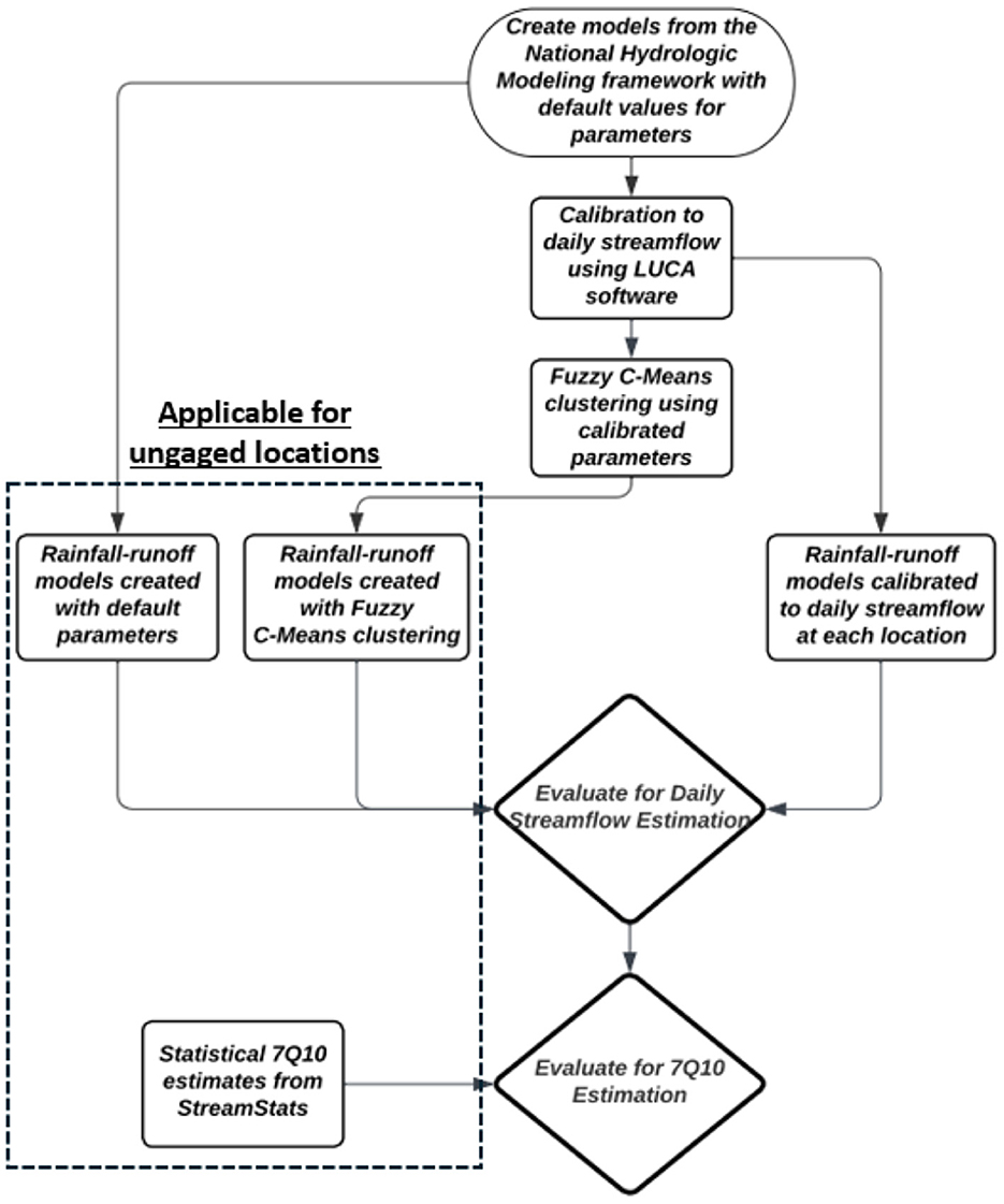
Figure 1. Summary of this study's experimental design.
The results from this experiment will answer the following questions:
(1) Do uncalibrated rainfall-runoff models, created using extractions from the USGS' National Hydrologic Modeling framework, perform comparably to regression-based 7Q10 estimation?
(2) Can models calibrated using Fuzzy C-Means clustering provide improved 7Q10 estimation compared to publicly available regression models?
2 Data and study area
The following sections describe the study area (Section 2.1) and data used in this research (Section 2.2).
2.1 Study area
The study area for this analysis is the northeast United States, including the states of Maine, New Hampshire, Vermont, Massachusetts, Rhode Island, Connecticut, New York, Pennsylvania, New Jersey, Delaware, Maryland, Virginia, and West Virginia. This area is roughly 260,000 square miles and is not homogenous, as it covers two distinct Hydrologic Unit Code (HUC) regions of the U.S. (Seaber et al., 1987). Basins selected for this study have been defined as “unimpaired” in USGS's Hydro-Climatic Data Network, HCDN-2009 (Lins, 2012). This set of stream gages includes 94 watersheds of varying size and physical attributes. These basins range from 2.1 mi2 to 1,419 mi2 (Figure 2).
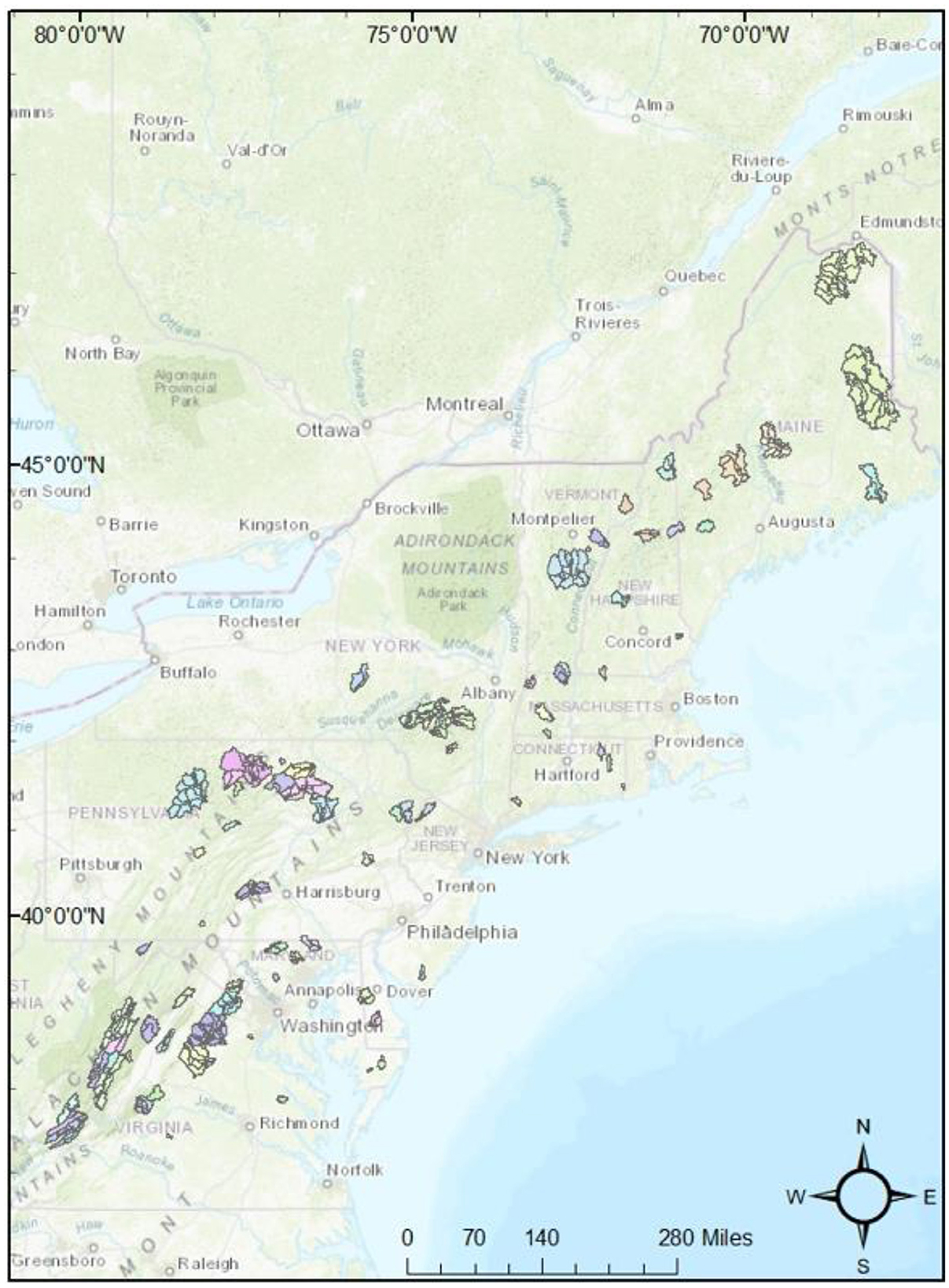
Figure 2. A 94 unimpaired gaged basins in the Northeast United States.
2.2 Data
2.2.1 Streamflow and 7Q10 data
Streamflow data from these 94 gages were downloaded from the USGS's Current Water Data for the Nation (https://waterdata.usgs.gov/nwis/rt). For this experiment, the full record of streamflow was used for calculation of the 7Q10 at each site. The “fasstr” software package (https://cran.r-project.org/web/packages/fasstr/index.html) was used to calculate the 7Q10 directly from the daily streamflow data. This package applies a quantile distribution to daily streamflow data allowing for the efficient calculation of low flow frequency analysis metrics, including the 7Q10. These 7Q10 values were identical to the 7Q10 values calculated by the USGS at each site, presented on the USGS's StreamStats Data-Collection Station reports (https://streamstatsags.cr.usgs.gov/).
2.2.2 Process-based hydrologic models
Rainfall-runoff models for each of the 94 gaged locations were extracted from the USGS's National Hydrologic Model version of the Precipitation Runoff Modeling System (NHM-PRMS). The USGS National Hydrologic Model (NHM) infrastructure was developed to support the efficient creation of local, regional, and national-scale hydrologic models for the United States (Regan et al., 2019). These models incorporate data stored in the NHM, including the basin and subbasin landcover values and area-weighted average climate forcings required to run PRMS. Selecting a location or gage that is a point-of-interest in the NHM generates a ready-to-run rainfall-runoff model at that location, with all necessary variables being extracted for the basin of interest, including land data (area, elevation, landcover) and the corresponding climate data. Climate forcing dataset choices include Daymet (1980–2016) (Thornton et al., 2016), Maurer (1949–2010) (Maurer et al., 2002), and Livneh (1915–2015) (Livneh and National Center for Atmospheric Research Staff, 2019) in the form of basin area-weighted precipitation and temperature timeseries. For this analysis, the Daymet climate dataset was chosen because it offers the finest resolution of the three (1 km, as opposed to 6 km for Livneh and ~12 km for Maurer) and allows for trend analysis, as there are no temporal discontinuities.
Additionally, the NHM-PRMS makes several major assumptions to model hydrologic processes. This includes:
1. Dividing basins into subbasins using pre-determined Hydrologic Response Units (HRUs) from the USGS' Geospatial Fabric (Bock et al., 2020).
2. Using a daily time-step, while some models utilize finer timesteps.
3. Calculating evapotranspiration using the Jensen-Haise (JH) formulation (Jensen and Haise, 1963).
The assumptions above are specific to the NHM-PRMS but should not imply that the results from this study will be specific to this hydrologic modeling software. The HRUs from the NHM-PRMS are based on pre-determined areas of homogeneity. Though some other models utilize gridded landcover data, all of the gridded values that would fall within an HRU should be similar to the value used for that HRU from the NHM-PRMS. Using a daily time-step may provide inaccurate high-flow estimates, as things like the 100-year-flood are calculated using gage data on a 15-min scale when it is available (England et al., 2019), but the 7Q10 is always calculated from daily average streamflows. Calculating evapotranspiration using the JH formulation may have an impact on results, but the appropriate steps have been taken to minimize the impact. JH calculates evapotranspiration based on temperature for each HRU. In this study, the Daymet climate dataset is used, which provides the finest resolution of the available climate datasets with no discontinuities. Additionally, extensive model calibration is used to minimize the impact of the JH formulation. JH is calibrated during its own step of the standard NHM calibration procedure, which will be further described in Section 3.1.
2.2.3 StreamStats 7Q10 estimates
To compare 7Q10 estimates from the process-based hydrologic models to current statistical estimates, the USGS's statistical estimation program StreamStats is used. StreamStats was chosen for comparison because (1) it is widely utilized by resource managers in the study area, (2) it provides direct comparisons, and (3) it utilizes a statistical methodology for estimation, as opposed to another process-based methodology. Without estimating daily streamflow, this program uses multiple linear regression equations, derived in log-space, to directly estimate flow statistics (Ries et al., 2008). Though the input variables vary by state, the typical process is as follows:
1. Calculate the historic 7Q10 at various gaged locations in a homogenous hydrologic area.
2. Collect the physical characteristics (watershed area, elevation, slope, etc.) for each of the watersheds attributed to the gages used above.
3. Fit a multiple linear regression, in log-space, to relate the input variables (watershed area, elevation, slope, etc.) to the corresponding 7Q10 value.
4. Delineate the watershed that is attributed to the ungaged location of interest.
5. Calculate the physical characteristics of the delineated watershed.
6. Apply the physical characteristics from the ungaged, delineated watershed to the regression equation developed in step 3 to calculate the 7Q10.
StreamStats uses varying regression equations and explanatory variables for Massachusetts (Ries, 2000), Rhode Island (Bent et al., 2014), New Hampshire (Flynn and Tasker, 2002), Maine (Dudley, 2004), Pennsylvania (Stuckey, 2006), Virginia (Austin et al., 2011), and West Virginia (Wiley, 2008). StreamStats 7Q10 has not been developed in Connecticut, Delaware, Maryland, New Jersey, New York, and Vermont, which partially limits later comparisons.
3 Methodology
In the following section, all methods used in this research are described in detail. This includes calibration of the NHM-PRMS models (Section 3.1), Fuzzy C-Means clustering for regionalization (Section 3.2), Silhouette Analysis for evaluating the optimal number of clusters (Section 3.3), and the evaluation metrics used for both the daily streamflow models and 7Q10 estimates (Section 3.4).
3.1 Calibration of the NHM-PRMS models
Models of the 94 basins were calibrated using the procedure recommended in the PRMS IV Manual (Markstrom et al., 2015) by executing the USGS's automated calibration software LUCA (Hay and Umemoto, 2007). This procedure applies a multi-objective, multi-step process of continuously revising sub-basin parameters. To achieve calibration, parameters are varied individually for each of the 94 locations, with the objective of minimizing the difference between the simulated daily streamflow and the measured daily streamflow at each gage. The parameters recommended for calibration in PRMS are summarized in Table 1, along with their default values and recommended calibration bounds (Markstrom et al., 2015).
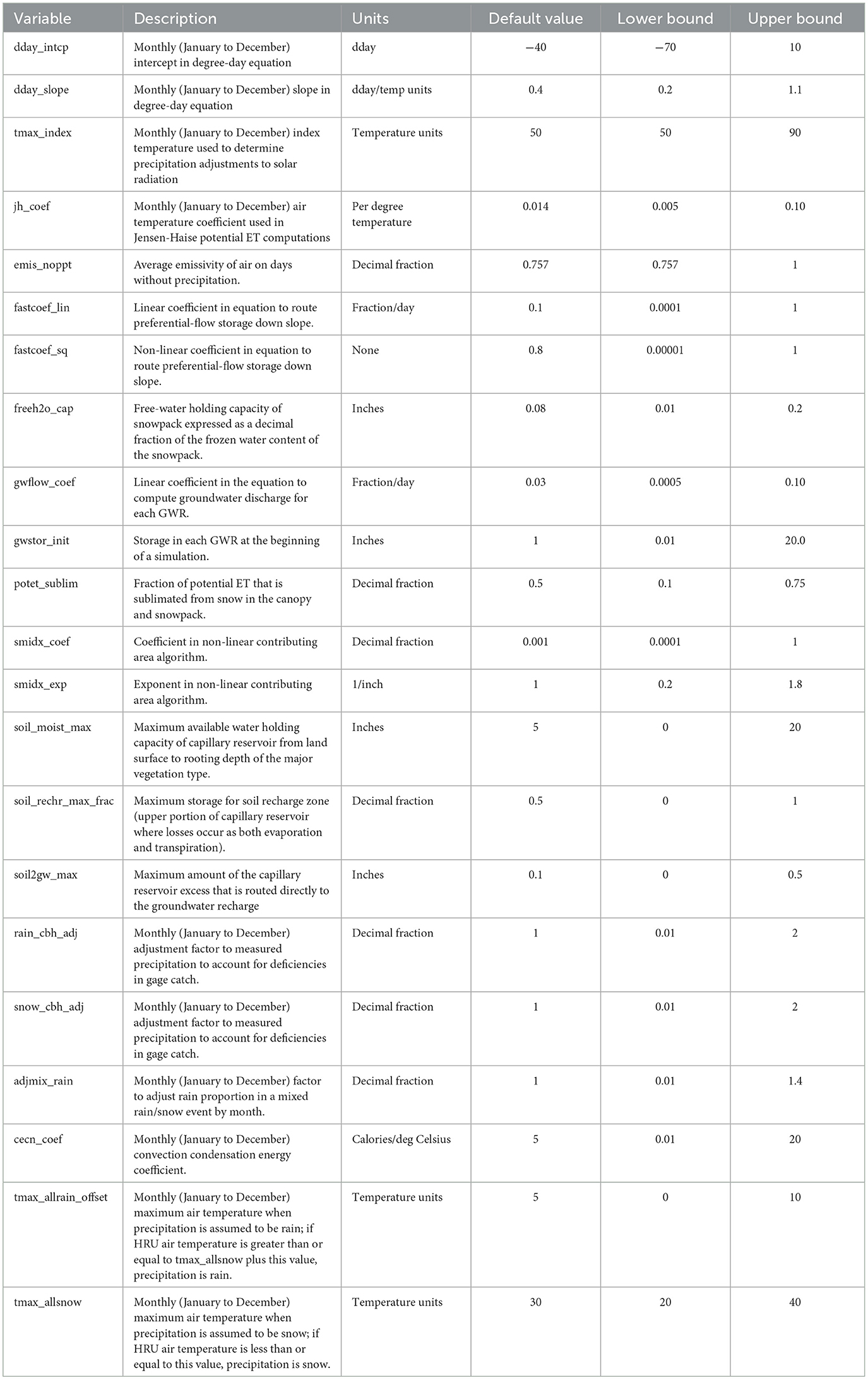
Table 1. Parameters calibrated in the process-based hydrologic model.
Each parameter that is to be calibrated begins with the default value and is continually refined during the calibration process. During calibration, the parameters are constrained to lie within the process-driven limits given above. In preparation for clustering, the updated values of the parameters are normalized using standard min-max normalization:
Figure 3 displays the range of parameters values after calibration and normalization. Normalization causes all the parameters to share the same range of 0 to 1. These values can easily be returned to their actual values by using the minimum and maximum values given below each boxplot in Figure 3 and reversing the equation above to solve for x.
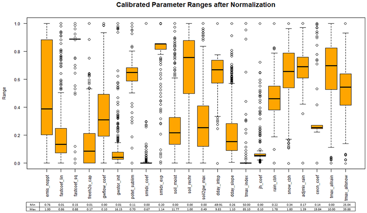
Figure 3. Parameter ranges after calibration and min-max normalization.
Calibration of the rainfall-runoff models was initially set up to minimize the error for low-flow estimation rather than for daily streamflows, deviating from the recommended calibration procedure in the PRMS IV manual (Markstrom et al., 2015). This was considered appropriate because the goal of this experiment is to test hydrologic models for low flow estimation. Specifically, the LUCA software allows for calibration to the lowest annual daily streamflows. Initial results suggested that the rainfall-runoff models calibrated to low flows were able to estimate the magnitude of 7Q10s well, but a more thorough analysis of the hydrograph suggested that the models were not properly maintaining the water budget and corresponding streamflow throughout the rest of the year. This discrepancy is highlighted in Appendix A, which highlights gage 01552000 in Pennsylvania on Loyalsock Creek as an example.
3.2 Fuzzy C-Means clustering
Traditional calibration of a rainfall-runoff model to daily streamflow is only possible at gaged locations. Furthermore, at these locations, 7Q10s can be directly calculated from the measured streamflow data. However, to extend calibration to ungaged locations, hydrologic regionalization can be used to transfer model parameters. Fuzzy C-Means (FCM) clustering is a clustering algorithm that utilizes soft assignments of data points to clusters (Dunn, 1973). Unlike traditional clustering algorithms like K-means clustering (MacQueen, 1967) that create hard assignments for each data point to a single cluster, FCM assigns membership values to indicate the degree of “belongingness” of data points to each cluster. The objective function seeks to find the optimal cluster centers and membership values that minimize the overall fuzziness or uncertainty of the clustering result. The FCM algorithm provides greater flexibility in clustering tasks, as it can handle scenarios where data points may partially belong to multiple clusters or where cluster boundaries are ambiguous. This is advantageous in this application, as this methodology is tested for a large geographical area that includes two pre-determined HUC regions of the United States. By assigning membership values, FCM provides a more nuanced representation of the clustering structure and allows for capturing overlapping clusters or gradual transitions between clusters. These membership values were used to create a weighted average of the parameters to use in the rainfall-runoff models. This is illustrated in Figure 4.
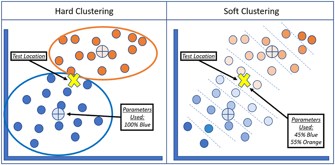
Figure 4. Difference between hard clustering algorithms (e.g., K-Means) and soft clustering algorithms (e.g., Fuzzy-C Means).
For implementation, a value “m” is used to set the “fuzzification” factor, dictating how much overlap to allow between clusters. As m is increased, the allowed overlap between clusters is increased. The FCM algorithm is executed for the total number of clusters possible with a specified range of m-values. The range of clusters possible for FCM is integers between [2, N/2] (for this case between 2 and 262), as there are 525 individual sub-basins with their own set of parameters. The range of m values possible is [1.5, ∞]. In this study, m values of [1.5, 5] will be used with increasing steps of 0.10. This will test 36 different m values for each cluster, leading to a total number of 9,396 possible cluster and fuzziness combinations for this experiment. Note that when m = 1, there is no overlap allowed between clusters and FCM reduces to K-Means clustering.
Clustering algorithms are typically used descriptively to highlight patterns in a dataset, but they can be used prescriptively given a set of predictor variables and response variables. For this study, the response variables for the FCM clustering are the calibrated parameters given in Table 1, as that is what must be predicted for calibrating the models at ungaged locations. The predictor variables, which will be used to predict which set of calibrated parameters to use, are the publicly available physical parameters for each sub-basin from the NHM, all designated as numeric values. These are highlighted in Table 2.
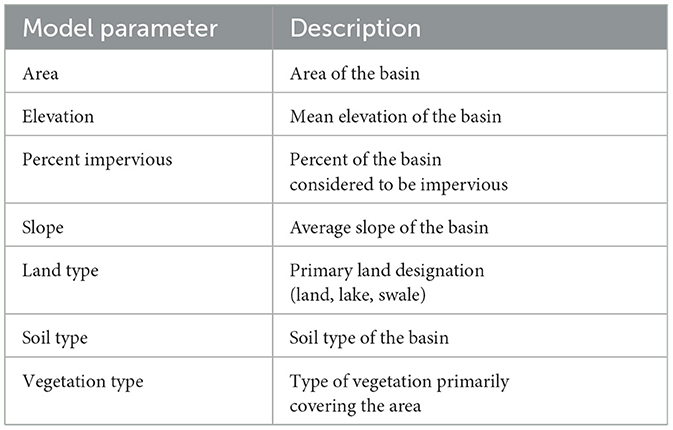
Table 2. Predictor variables used in the Fuzzy C-Means analysis from the 94 test basins.
Given the above parameters, the process for creating the new models using Fuzzy C-Means is summarized below.
1. Calibration creates response variables (Table 1) for each location.
2. Predictor variables (Table 2) are extracted from each location.
3. All parameters are normalized using min-max normalization (Equation 1).
4. Clustering is used to create groups of similar basin parameters 1.
5. Fuzzy C-Means clustering is used to evaluate each location's membership to each group.
6. New calibrated parameters are created using a weighted average of each location's membership to each cluster and the cluster's corresponding centroid (Figure 4).
The FCM algorithm is known to suffer from several drawbacks, including computational time complexity, initial cluster centers, membership matrix reliance, and noise sensitivity. In this study, strategic measures were implemented to mitigate these drawbacks effectively. To address the issue of computational time complexity, parallel computing techniques were utilized to ensure efficient execution. To overcome the sensitivity to initial cluster centers, a robust initialization strategy was employed to integrate multiple runs with distinct initializations to determine the configuration that yielded optimal results. Additionally, the membership matrix was manually evaluated and refined to enhance the stability of the clustering process and minimize the impact of noise. These approaches aim to mitigate the various drawbacks of the FCM method and improve the robustness of the clustering methodology.
3.3 Silhouette analysis
Silhouette analysis (Rousseeuw, 1987) is a common methodology used for calculating the optimal number of clusters for a dataset. This methodology evaluates the quality of clustering by assessing the separation and cohesion of clusters, as well as the fit of data points within their assigned clusters (Rousseeuw, 1987). First, a silhouette coefficient is calculated for each data point that measures how well it fits within its cluster compared to neighboring clusters. Next, the average silhouette coefficient is computed across all data points for each value of the number of clusters. Finally, the optimal number of clusters is determined by selecting the value that maximizes the average silhouette coefficient, indicating the presence of well-separated and compact clusters.
Silhouette analysis was chosen to determine the optimal number of clusters due to its ability to quantify both cohesion and separation within clusters. Unlike other techniques for determining the optimal number of clusters, this method provides a clear and intuitive measure of the quality of clustering, considering both the compactness of clusters and their distinctiveness. Its versatility allows for the evaluation of clustering performance across varying cluster configurations, making it a well-suited metric for this study where the identification of an optimal cluster number is crucial for optimizing the rainfall-runoff models. For this experiment, models created from the parameter clusters are executed with the four highest average silhouette coefficients. Because parameters are regionalized for use in a rainfall-runoff model, there may be some slight variations between the cluster/m-value combination with the best average silhouette coefficient and the rainfall-runoff model with the optimal daily streamflow. By testing four models, the link between the optimal silhouette coefficients and optimal physical model performances can be verified, as well as ensuring that the single model with the best daily streamflow and 7Q10 estimation is identified. If the silhouette analysis suggests that there are distinct clusters, which would occur if the highest average silhouette coefficients occur when m = 1.5 (the smallest fuzzification factor possible) and decrease as m is incrementally increased, models with m = 1 should also be tested, which would reduce the FCM to K-Means clustering.
3.4 Evaluation metrics for daily streamflow and 7Q10 estimates
In this experiment, the Kling Gupta Efficiency (KGE) (Gupta et al., 2009) is used to evaluate the daily streamflow models. KGE is widely used for hydrologic applications (Formetta et al., 2011; Beck et al., 2016) because it incorporates three components into its definition: the Pearson's correlation coefficient (r), the bias (β), and the error variability (α). KGE is calculated using the following formula (Equation 2):
Unlike traditional metrics like R2 (Wright, 1921) and Nash-Sutcliffe Efficiency (NSE) (Nash and Sutcliffe, 1970), KGE considers three key components of model performance: correlation, bias, and variability, which combined offer a holistic assessment of model fit. This provides a nuanced understanding of the model's ability to capture not only the mean and variability of the observed data, but also the temporal dynamics.
The goal of this experiment is to evaluate the models for 7Q10 estimation, so four error metrics will be used to evaluate the errors for 7Q10 estimation. These are Relative Bias (Equations 3–6),
Root Mean Square Error (RMSE),
Relative Root Mean Square Error (R-RMSE),
and Unit-Area RMSE (UA-RMSE),
where yi is the observed 7Q10, ŷ is the model predicted 7Q10, n is the total number of sites, DA is the drainage area, and is the associated mean value. Similar studies have also chosen RMSE over MAE for its sensitivity to outliers (Mekanik et al., 2016; Ferreira et al., 2021). These four metrics were chosen to complement each other and provide a comprehensive analysis of performance. RMSE provides a standard error estimate, while relative RMSE provides an error estimate adjusted for the mean of the dataset. Additionally, relative bias provides a direct bias estimate in relation to the size of the value itself, and Unit-Area RMSE adjusts RMSE for the size of the basin being analyzed. These additional metrics attempt to weight 7Q10 estimation in small basins and large basins similarly, where a bias estimate may be heavily skewed by the size of the values themselves (e.g., a 7Q10 estimate of 1.00cfs when the actual value is 0.00cfs, compared to a 7Q10 estimate of 100.00cfs when the actual value is 99.00cfs).
4 Results and discussion
The following sections present and discuss the uncalibrated model vs calibrated model performance for daily streamflow estimation (Section 4.1) and 7Q10 estimation (Section 4.2), the results from the silhouette analysis (Section 4.3), applying the optimal silhouettes with Fuzzy C-Means regionalization for daily streamflow estimation (Section 4.4), and the results of using the models calibrated using FCM for 7Q10 estimation (Section 4.5).
4.1 Uncalibrated model performance vs. calibrated model performance
In Figure 5, the general results for the uncalibrated rainfall-runoff models directly from the NHM-PRMS, compared to the calibrated models, are presented.
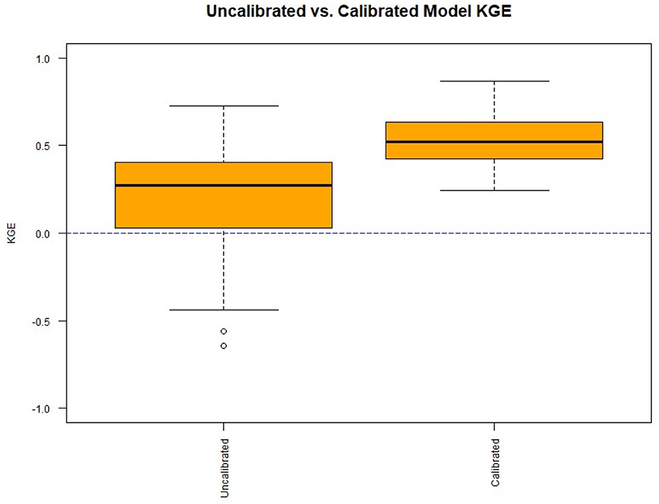
Figure 5. Results from calibration using KGE to evaluate daily streamflow estimation.
As expected, calibration improved daily streamflow estimation for every basin. Before calibration, the median KGE was 0.30 with some locations having negative KGE values. Calibration improved the median daily streamflow to 0.52, with the lowest KGE value being 0.25. The results are further analyzed by spatially disaggregating the basins into small (< 100 mi2) and large basins (>100 mi2). This threshold is chosen because many regression equations used for 7Q10 estimation, including some of the StreamStats' equations in the study area, are only recommended for basins up to 100–150 mi2 (e.g., Ries, 2000). Figures 6A, B display the physical model KGEs, but this time split by small basins (Figure 6A) and large basins (Figure 6B).
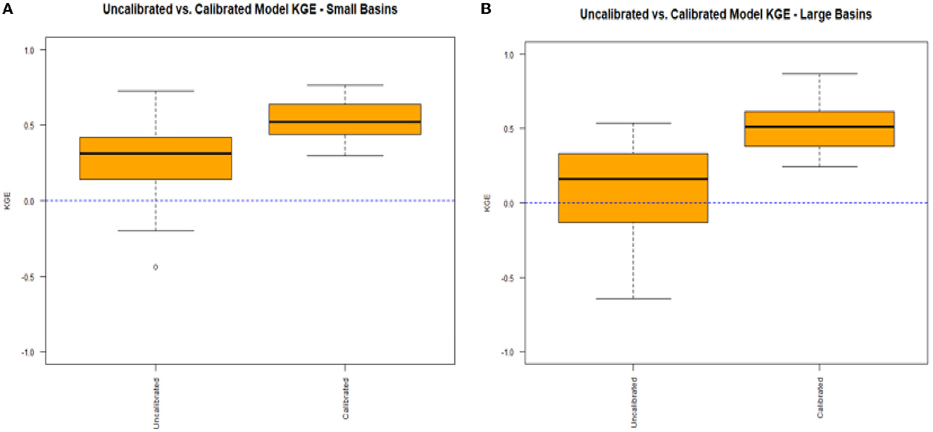
Figure 6. Results from calibration for basins smaller than 100 mi2 (A) and basins larger than 100 mi2 (B) using KGE to evaluate daily streamflow estimation.
There are minimal differences between the calibrated models for small and large basins, but the uncalibrated models display noticeable differences. The uncalibrated models for larger basins display an inferior median KGE, more KGE values that are negative, and a much wider interquartile range with a lower 25th percentile that is negative. The uncalibrated models for the larger basins perform significantly worse than the uncalibrated models for the smaller basins in terms of KGE. Given that the calibrated models for the large basins perform similarly to the calibrated models for the small basins, this suggests that the default parameter values are not as appropriate for larger basins, requiring calibration more than that of the models for small basins.
4.2 Uncalibrated vs. calibrated models for gaged 7Q10 estimation
This experiment's primary goal is to test the hypothesis that models can be used for 7Q10 estimation in ungaged locations. Of the 94 basins in the study, an estimate of the 7Q10 is not available through StreamStats for 28 of the basins (StreamStats 7Q10 estimation has not been developed by the USGS for certain states, as discussed in Section 2.2.3). These locations were removed from the analysis for the analyses presented in Sections 4.2 and 4.4. Table 3 summarizes the Median Relative Bias, RMSE, RRMSE, and UA-RMSE of the uncalibrated and calibrated models for 7Q10 estimation compared to StreamStats.
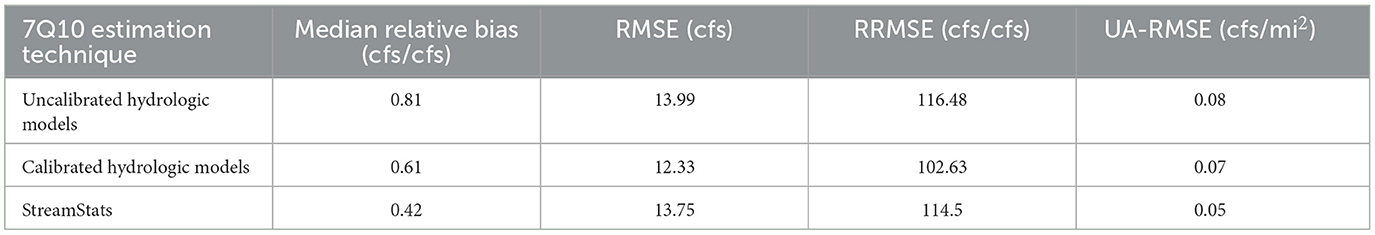
Table 3. Error metrics for 7Q10 estimation (only StreamStats locations).
For the 66 basins where StreamStats 7Q10 estimation is available, the results suggest that StreamStats provides significantly lower median relative bias and UA-RMSE to the uncalibrated models, but similar RMSE and RRMSE. The calibrated models perform best in terms of RMSE and RRMSE but provide significantly larger median relative bias and UA-RMSE than StreamStats. RMSE is heavily influenced by larger values, while UA-RMSE attempts to weigh smaller and larger values equally by scaling the larger values down based on their larger watershed areas. Because the calibrated models perform best for RMSE but not for UA-RMSE, this suggests that the calibrated models perform well for larger basins. Table 4 confirms this by displaying the same metrics characterized by small and large basins, defined in Section 4.1.
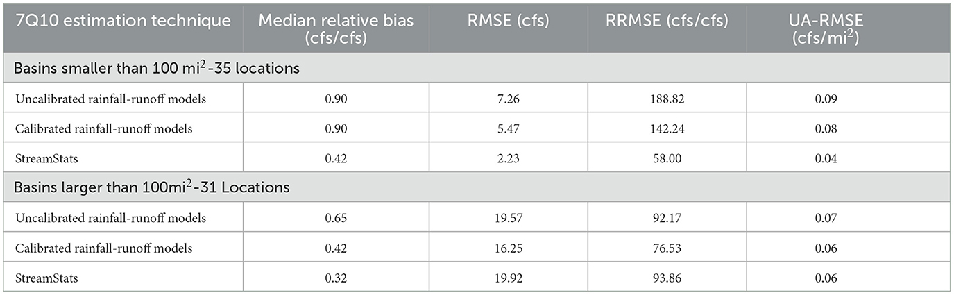
Table 4. Error metrics for 7Q10 estimation (only StreamStats locations).
Table 4 suggests that StreamStats outperforms both the uncalibrated and calibrated physical models for 7Q10 estimation in small basins. For the small basins, StreamStats' median relative bias, RMSE, RRMSE, and UA-RMSE are all half that (or more) of the calibrated models. For the large basins, StreamStats still performs best in terms of median relative bias, but the calibrated models display the same UA-RMSE and better RMSE and RRMSE than StreamStats. Given the results presented here, the calibrated physical models at gaged locations over 100 square miles can provide similar errors for 7Q10 estimation compared to StreamStats in terms of the error metrics presented, but StreamStats is primarily for ungaged basin estimation, and this calibration methodology cannot be used for ungaged locations. In the next section, a methodology is presented for calibrating models in ungaged locations using Fuzzy C-Means clustering for hydrologic regionalization.
4.3 Results from silhouette analysis with Fuzzy C-Means clustering
As summarized in Section 3.3, silhouettes were used to find the optimal FCM parameters. The full range of clusters possible are combined with m-values ranging from 1.5 to 5 using steps of 0.1. Figure 7 displays the average silhouette widths for each combination of clusters and m-values.
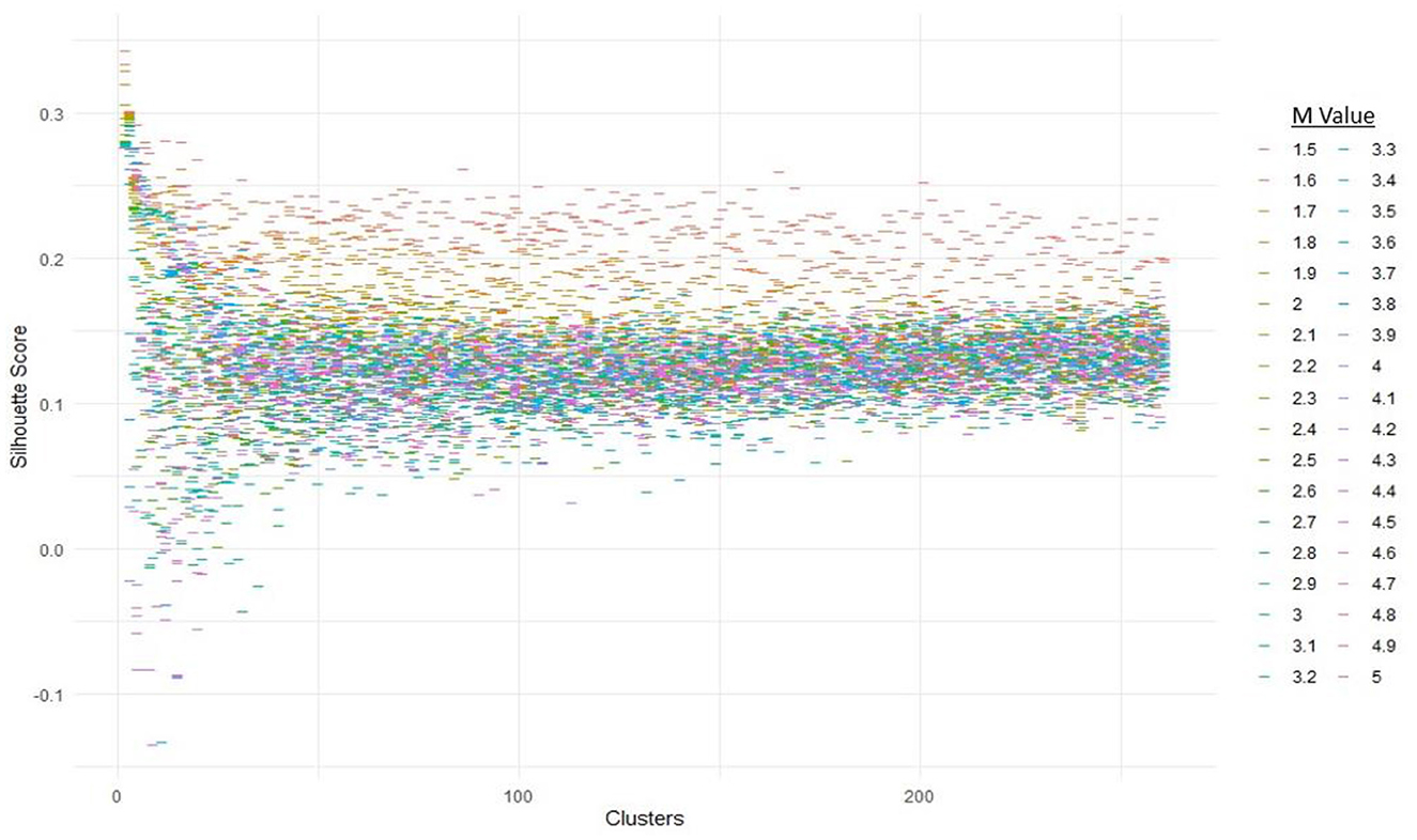
Figure 7. Silhouette analysis for the Fuzzy C-Means clustering.
In addition, the top 10 average silhouette coefficients, arranged from largest to smallest, are presented in Table 5.
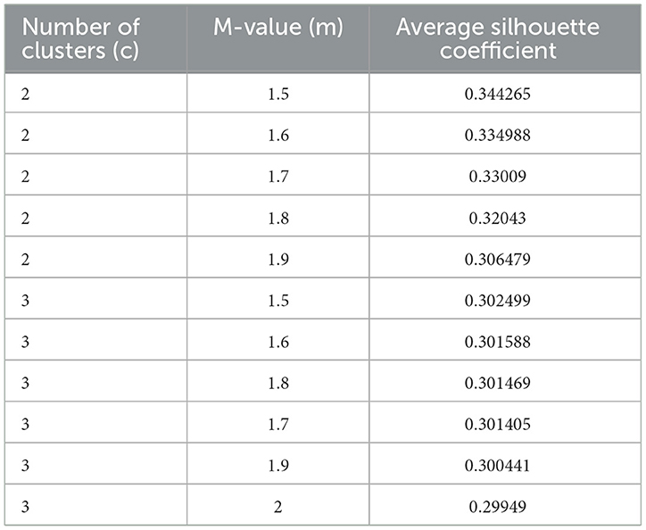
Table 5. Highest 10 average silhouette coefficients.
Results suggest that the cluster and m-value combination that optimizes the average silhouette coefficient is the minimum value for both clusters and m. The best average silhouette coefficient was found to occur when c = 2 clusters with an m-value of 1.5. The next 4 best silhouette coefficients remain when c = 2 but decrease slightly as m is increased by 0.10 each step. The next optimal number of clusters was found to be c = 3 for the 5th highest average silhouette coefficient, with the minimum m-value of 1.5 once again being optimal. When the number of clusters equals 3, the silhouette coefficients decrease slightly as m is increased by 0.10 each step once again. The results in Figure 7 and Table 5 suggest that there may be distinct clusters that need to be considered. Exemplified by the results in Table 5 but can also be seen in Figure 7, the silhouette coefficients decrease as the m-value is increased, suggesting less optimal solutions as the fuzziness between clusters is increased. For both clusters c = 2 and c = 3, the smallest m-value displayed the best average silhouette coefficient.
Based on the results from Figure 7 and Table 5 that suggest possible distinct clusters, rather than test the four parameter combinations which display the best average silhouette coefficient (which would be when c = 2 and m = 1.5, 1.6, 1.7, and 1.8), the following four models will be tested:
1. FCM when c = 2 and m = 1 (reduces to K-Means clustering where k = 2).
2. FCM when c = 2 and m = 1.5 (FCM for c = 2 with the minimum fuzziness factor m = 1.5).
3. FCM when c = 3 and m = 1 (reduces to K-Means clustering where k = 3).
4. FCM when c = 3 and m = 1.5 (FCM for c = 3 with the minimum fuzziness factor m = 1.5).
This will allow us to test: (1) the optimal result from the silhouette analysis (c = 2 and m = 1.5), (2) multiple clusters (c = 2 and c = 3), and (3) whether applying distinct clusters leads to better calibration, as suggested by the silhouettes.
4.4 Results from clustering for daily streamflow
New rainfall-runoff models were created using clustering for the four scenarios discussed in the previous section. Figure 8 summarizes how each model created from clustering performs for daily streamflow estimation.
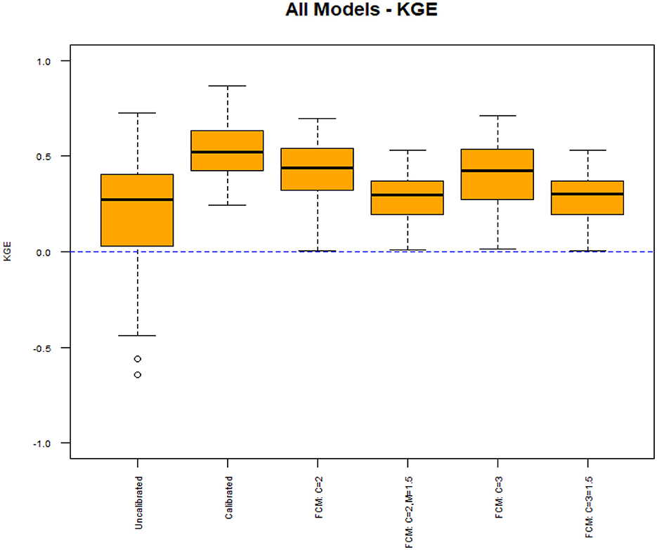
Figure 8. Daily streamflow KGE using FCM for calibration.
Figure 8 shows that some models calibrated using FCM display improved KGEs compared to the uncalibrated models. Both models with no fuzzification factor (FCM: C = 2 and FCM: C = 3) display median KGEs slightly below 0.50, while the models with a fuzzification factor (FCM: C = 2, M = 1.5, and FCM: C = 3, M = 1.5) display median KGEs around 0.30. Even with this improvement however, there are some locations that have a KGE close to 0 for all four models calibrated with FCM. All models calibrated using FCM display minimum KGEs close to 0, but this is still an improvement compared to the uncalibrated models where the 25th percentile KGE is just above 0. The models created with a fuzzification factor of m = 1.5 display much poorer median KGEs than the models created with distinct clusters. The results from silhouette analysis suggested that distinct clusters may provide more optimal solutions, and the results from Figure 6 support that using distinct clusters improves KGE significantly more on average than the models created with fuzzification factors.
In Figures 9A, B, the models are once again separated by area for further analysis.
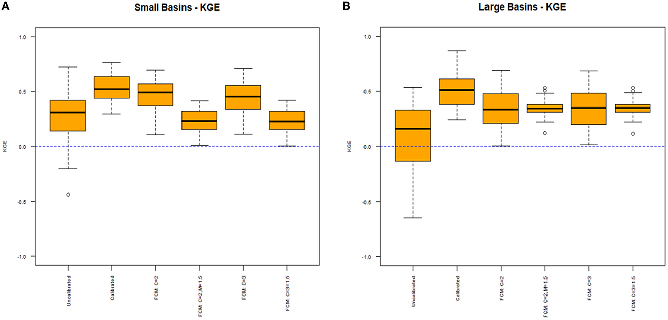
Figure 9. Results from calibration for basins smaller than 100 mi2 (A) and basins larger than 100 mi2 (B) using KGE to evaluate daily streamflow estimation.
The results from Figures 9A, B provide further explanation for the general results given in Figure 8. Figure 9A shows that results for the smaller basins are very similar to the overall results given in Figure 8, that models calibrated with distinct clusters once again provide only slightly poorer median KGEs than the model calibrated to daily streamflow at each location. It also supports that using distinct clusters provides significant improvement compared to using a fuzzification factor. However, Figure 9B shows that for the larger basins, all models created using clustering (with or without a fuzzification factor) display almost the same median KGE of about 0.30. The models created using a fuzzification factor even display slightly higher median KGEs, with smaller interquartile ranges and better minimum KGEs. Overall, results from Figures 9A, B suggest that distinct clusters should be used when creating physical models for smaller basins (< 100 mi2), but for larger basins (>100 mi2), adding a fuzzification factor may provide similar results on average but less variability.
Next, the models are evaluated specifically for their ability to estimate 7Q10s.
4.5 Procedure for optimal cluster selection for overall model performance
Similar to Section 4.2, an analysis of all models for 7Q10 estimation is provided in Table 6.
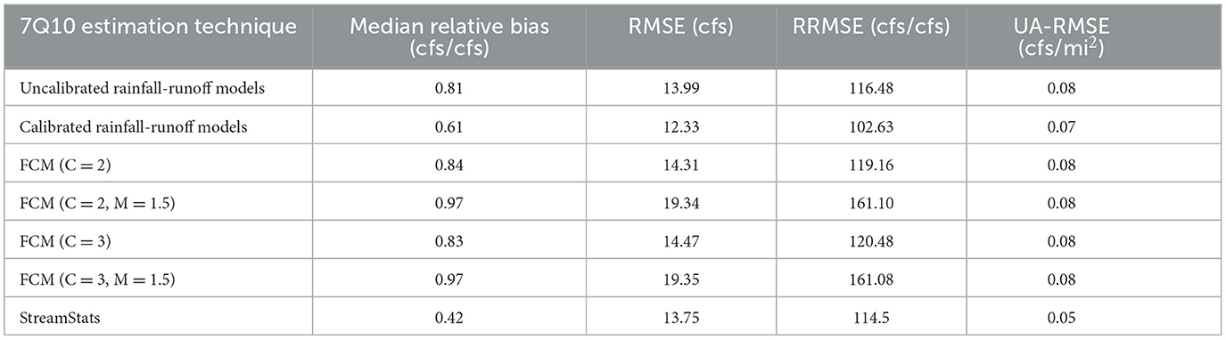
Table 6. Error metrics for 7Q10 estimation (only StreamStats locations).
The results from Table 6 suggest that even with the improvement for daily streamflow estimation shown in Section 4.4, none of the models provide better median relative bias, RMSE, RRMSE, or UA-RMSE compared to StreamStats. The models created using distinct clusters provide slightly higher RMSE and RRMSE than StreamStats but provide substantially higher relative bias and UA-RMSE. This is further analyzed in Table 7, which separates small and large basins for analysis.
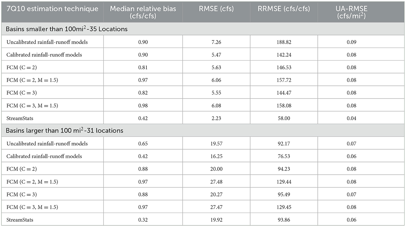
Table 7. Error metrics for 7Q10 estimation (only StreamStats locations).
Table 7 shows that for small basins, StreamStats provides the best 7Q10 estimation by far for all metrics employed. In terms of median relative bias, RMSE, RRMSE, and UA-RMSE, StreamStats' estimates provide roughly half of the error compared to all other methods. For larger basins however, results are much more mixed. StreamStats does provide the best median relative bias by far, but for all other metrics, the calibrated models and models created with no fuzzification factor perform comparably to StreamStats for 7Q10 estimation. The calibrated models provide better RMSE and RRMSE, as well as an identical UA-RMSE. The models created using FCM with no fuzzification factor also display comparable but slightly larger RMSE, RRMSE, and UA-RMSE than StreamStats.
In Figures 10A–D, a plot of the 7Q10 bias for each model is provided. Bias is calculated by [estimated–actual], meaning points above the 0 line suffer from overestimation and points below suffer from underestimation. The corresponding line through the points follows a loess smoothing curve (https://www.rdocumentation.org/packages/stats/versions/3.6.2/topics/loess) with the corresponding standard error highlighted in gray. This provides those interested in using these models for 7Q10 estimation with three valuable insights:
1. For any of the models, the average bias that can be expected with a basin area of X.
2. The corresponding confidence in that estimate, given by the highlighted area.
3. If any of the models are consistently overestimating or underestimating 7Q10s for a range of basin sizes.
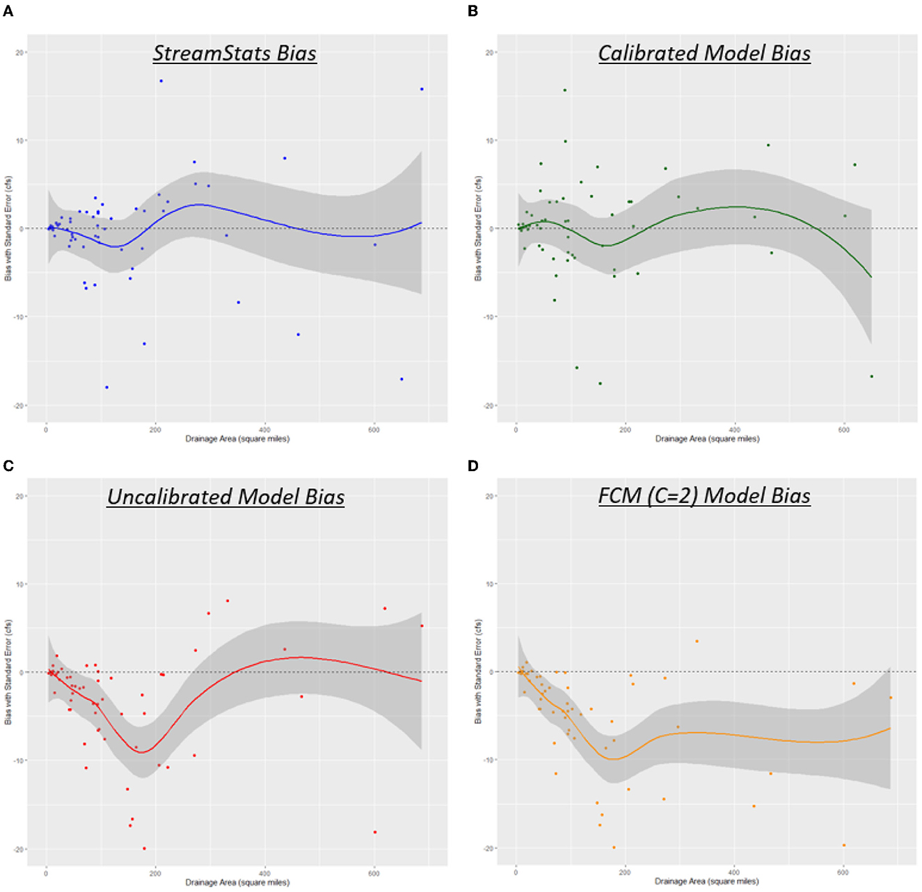
Figure 10. (A–D) Bias created from each model used, arranged by drainage area.
For both StreamStats and the calibrated models, the average bias remains around 0 for all range of basin sizes. There seems to be some minimal oscillation that suggests slight overestimation or underestimation depending on the basin size, but 0 remains in the highlighted confidence interval for the full range of basin sizes. For the uncalibrated models and models created using FCM (C = 2), there are clear patterns that demonstrate weaknesses in these modeling approaches. The uncalibrated models are heavily underestimating 7Q10s for basin sizes that range from 50–250 mi2, and the models calibrated with FCM (C = 2) are consistently underestimating 7Q10s for basins larger than 50 mi2. Given the results in Table 7 and Figures 10A–D, the only physical models that provide sufficient
7Q10 estimation are the individually calibrated hydrologic models, which cannot be used in ungaged basins.
5 Conclusions
Based on the results from this experiment, the results support that resource managers who require 7Q10 estimates in gaged basins can use calibrated models in basins larger than 100 mi2 and expect similar errors to current statistical estimates. For basins smaller than that, statistical estimates still provide smaller median relative bias, RMSE, RRMSE, and UA-RMSE for 7Q10 estimation. 7Q10s in these smaller basins can be extremely small values, however, and it should be considered how accurate estimates need to be to be sufficient for their exact design application. For example, the 7Q10 is frequently used in wastewater treatment plant design as a mixing flow. Though it is difficult to attribute exact costs to value changes, an estimated mixing flow of 1.00 cfs could cause a significantly different design than a mixing flow of 0.10 cfs, only having a difference of 0.90 cfs. However, in the case of a future climate change study where the accuracy of the value itself is less important than model-predicted future changes in the value, the process-based estimates readily allow for the incorporation of altered climate and/or landcover projections. Given few alternatives, the process-based models also provide the ability for resource managers to estimate 7Q10s in states where StreamStats 7Q10 estimation is not yet developed. Future work related to this study could include testing this procedure with other process-based models, determining other ways to calibrate physical models in ungaged locations for both daily streamflow and low flow estimation, and further analyzing the performance of physical models for gaged and ungaged high flow estimation (e.g., 100-year-flood estimation) as well.
Data availability statement
The original contributions presented in the study are included in the article/Supplementary material, further inquiries can be directed to the corresponding author.
Author contributions
AD: Writing—original draft. RP: Writing—review & editing. KA: Writing—review & editing.
Funding
The author(s) declare financial support was received for the research, authorship, and/or publication of this article. This research was funded by a U.S. Geological Survey Northeast Climate Adaptation Science Center award G21AC10556 and a decision support system for estimating changes in extreme floods and droughts in the Northeast U.S., to AD.
Acknowledgments
The authors thank Parker Norton and Jacob Lafontaine of the United States Geological Survey for providing hydrologic models using extractions from the National Hydrologic Modeling framework, access to the Let Us Calibrate Software, and initial advice on modeling steps.
Conflict of interest
The authors declare that the research was conducted in the absence of any commercial or financial relationships that could be construed as a potential conflict of interest.
Publisher's note
All claims expressed in this article are solely those of the authors and do not necessarily represent those of their affiliated organizations, or those of the publisher, the editors and the reviewers. Any product that may be evaluated in this article, or claim that may be made by its manufacturer, is not guaranteed or endorsed by the publisher.
Supplementary material
The Supplementary Material for this article can be found online at: https://www.frontiersin.org/articles/10.3389/frwa.2024.1332888/full#supplementary-material
References
Asquith, W. H., and Thompson, D. B. (2008). Alternative regression equations for estimation of annual peak-streamflow frequency for undeveloped watersheds in Texas using PRESS minimization. U.S. Geological Survey Scientific Investigations Report 2008–5084 p. 40. doi: 10.3133/sir20085084
Austin, S. H., Krstolic, J. L., and Wiegand, U. (2011). Low-flow characteristics of Virginia streams. U.S. Geological Survey Scientific Investigations Report 2011–5143 p. 122. doi: 10.3133/sir20115143
Ayers, J., Villarini, G., Jones, C., Schilling, K., and Farmer, W. (2022). The role of climate in monthly baseflow changes across the continental United States. J. Hydrol. Eng. 27, 2170. doi: 10.1061/(ASCE)HE.1943-5584.0002170
Bayazit, M. (2015). Nonstationarity of hydrological records and recent trends in trend analysis: a state-of-the-art review. Environ. Process. 2, 527–542. doi: 10.1007/s40710-015-0081-7
Beck, H. E., van Dijk, A. I. J. M., de Roo, A., Miralles, D. G., McVicar, T. R., Schellekens, J., et al. (2016). A Global-scale regionalization of hydrologic model parameters. Water Resour. Res. 52, 3599–3622. doi: 10.1002/2015WR018247
Bent, G. C., Steeves, P. A., and Waite, A. M. (2014). Equations for estimating selected streamflow statistics in Rhode Island. U.S. Geological Survey Scientific Investigations Report 2014–5010 p. 65. doi: 10.3133/sir20145010
Berghuijs, W. R., Woods, R. A., Hutton, C. J., and Sivapalan, M. (2016). Dominant flood generating mechanisms across the United States. Geophys. Res. Lett. 43, 4382–4390. doi: 10.1002/2016GL068070
Blum, A. G., Archfield, S. A., Hirsch, R. M., Vogel, R. M., Kiang, J. E., and Dudley, R. W. (2019). Updating estimates of low-streamflow statistics to account for possible trends. Hydrol. Sci. J. 64, 1404–1414. doi: 10.1080/02626667.2019.1655148
Bock, A. E., Santiago, M., Wieczorek, M. E., Foks, S. S., Norton, P. A., and Lombard, M. A. (2020). Geospatial Fabric for National Hydrologic Modeling, version 1.1 (ver. 3.0, November 2021). U.S. Geological Survey data release.
Boyle, D. P., Gupta, H. V., and Sorooshian, S. (2000). Toward improved calibration of hydrologic models: combining the strengths of manual and automatic methods. Water Resour. Res. 36, 3663–3674. doi: 10.1029/2000WR900207
Brunner, M. I., Slater, L., Tallaksen, L. M., and Clark, M. (2021). Challenges in modeling and predicting floods and droughts: a review. WIREs Water. 8, e1520. doi: 10.1002/wat2.1520
California Department of Water Resources (2021). Water Year 2021: An Extreme Year. Available online at: https://water.ca.gov/-/media/DWR-Website/Web-Pages/Water-Basics/Drought/Files/Publications-And-Reports/091521-Water-Year-2021-broch_v2.pdf (accessed September 9, 2023).
Castellarin, A. (2014). Regional prediction of flow-duration curves using a three-dimensional kriging. J. Hydrol. 513, 179–191. doi: 10.1016/j.jhydrol.2014.03.050
Champagne, O., Arain, M. A., Leduc, M., Coulibaly, P., and McKenzie, S. (2020). Future shift in winter streamflow modulated by the internal variability of climate in southern Ontario. Hydrol. Earth Syst. Sci. 24, 3077–3096. doi: 10.5194/hess-24-3077-2020
Driscoll, J. M., Hay, L. E., Vanderhoof, M., and Viger, R. J. (2020). Spatiotemporal variability of modeled watershed scale surface-depression storage and runoff for the conterminous United States. J. Am. Water Resour. Assoc. 56, 16–29. doi: 10.1111/1752-1688.12826
Duan, Q. (2003). “Global optimization for watershed model calibration,” in Calibration of Watershed Models, eds. Q. Duan, H. V. Gupta, S. Sorooshian, A. N. Rousseau, and R. Turcotte. doi: 10.1029/WS006
Dudley, R. W. (2004). Estimating Monthly, Annual, and Low 7-Day, 10-Year Streamflows for Ungaged Rivers in Maine. U.S. Geological Survey Scientific Investigations Report 2004-5026, p. 22. doi: 10.3133/sir20045026
Dunn, J. C. (1973). A fuzzy relative of the ISODATA process and its use in detecting compact well-separated clusters. J. Cybern. 3, 32–57. doi: 10.1080/01969727308546046
El Gharamti, M., McCreight, J. L., Noh, S. J., Hoar, T. J., RafieeiNasab, A., and Johnson, B. K. (2021). Ensemble streamflow data assimilation using WRF-Hydro and DART: novel localization and inflation techniques applied to Hurricane Florence flooding. Hydrol. Earth Syst. Sci. 25, 5315–5336. doi: 10.5194/hess-25-5315-2021
England, J. F., Cohn, T. A., Faber, B. A., Stedinger, J. R., Thomas, W. O., Veilleux, A. G., et al. (2019). Guidelines for determining flood flow frequency — Bulletin 17C (ver. 1.1, May 2019). U.S. Geological Survey Techniques and Methods, p. 148. doi: 10.3133/tm4B5
EPA Office of Water (2018). Low Flow Statistics Tools: A How-To Handbook for NPDES Permit Writers. https://www.epa.gov/sites/default/files/2018-11/documents/low_flow_stats_tools_handbook.pdf (accessed October 3, 2023).
Farmer, W. H., LaFontaine, J. H., and Hay, L. E. (2019). Calibration of the US geological survey national hydrologic model in ungauged basins using statistical at-site streamflow simulations. J. Hydrol. Eng. 24, 11. doi: 10.1061/(ASCE)HE.1943-5584.0001854
Ferreira, R. G., da Silva, D. D., Elesbon, A. A., Fernandes-Filho, E. I., Veloso, G. V., de Souza Fraga, M., et al. (2021). Machine learning models for streamflow regionalization in a tropical watershed. J. Environ. Manage. 280, 111713. doi: 10.1016/j.jenvman.2020.111713
Flynn, R. H., and Tasker, G. D. (2002). Development of Regression Equations to Estimate Flow Durations and Low-Flow-Frequency Statistics in New Hampshire Streams. U.S. Geological Survey Scientific Investigations Report 02-4298, p. 66.
Formetta, G., Mantilla, R., Franceschi, S., Antonello, A., and Rigon, R. (2011). The JGrass-New Age system for forecasting and managing the hydrological budgets at the basin scale: models of flow generation and propagation/routing. Geosci. Model Dev. 4, 943–955. doi: 10.5194/gmd-4-943-2011
Golian, S., Murphy, C., and Meresa, H. (2021). Regionalization of hydrological models for flow estimation in ungauged catchments in Ireland. J. Hydrol. 36, 100859. doi: 10.1016/j.ejrh.2021.100859
Guo, Y., Zhang, Y., Zhang, L., and Wang, Z. (2021). Regionalization of hydrological modeling for predicting streamflow in ungauged catchments: a comprehensive review. WIREs Water. 8, e1487. doi: 10.1002/wat2.1487
Gupta, H. V., Kling, H., Yilmaz, K. K., and Martinez, G. F. (2009). Decomposition of the mean squared error and NSE performance criteria: implications for improving hydrological modeling. J. Hydrol. 377, 80–91. doi: 10.1016/j.jhydrol.2009.08.003
Gupta, V., and Waymire, E. (1998). “Spatial variability and scale invariance in hydrologic regionalization,” in Scale Dependence and Scale Invariance in Hydrology, ed. G. Sposito (Cambridge: Cambridge University Press), 88–135. doi: 10.1017/CBO9780511551864.005
Hay, L., Norton, P., Viger, R., Markstrom, S., Regan, R. S., and Vanderhoof, M. (2018). Modeling surface-water depression storage in a Prairie Pothole Region. Hydrol. Proc. 32, 462–479. doi: 10.1002/hyp.11416
Hay, L. E., and Umemoto, M. (2007). Multiple-objective stepwise calibration using Luca. U.S. Geological Survey Open-File Report 2006–1323, p. 25. Available online at: http://pubs.usgs.gov/of/2006/1323/ (accessed March 22, 2023).
Hesarkazzazi, H., Arabzadeh, R., Hajibabaei, M., Rauch, W., Kjeldsen, T. R., Prosdocimi, I., et al. (2021). Stationary vs non-stationary modelling of flood frequency distribution across northwest England. Hydrol. Sci. J. 66, 729–744. doi: 10.1080/02626667.2021.1884685
Hodgkins, G. A., and Dudley, R. W. (2011). Historical summer base flow and stormflow trends for New England rivers. Water Resour. Res. 47, W07528. doi: 10.1029/2010WR009109
Hong, M., Zhang, R., Wang, D., Qian, L. X., and Hu, Z. H. (2017). Spatial interpolation of annual runoff in ungauged basins based on the improved information diffusion model using a genetic algorithm. Discr. Dyn. Nat. Soc. 18, 1–19. doi: 10.1155/2017/4293731
Hrachowitz, M., Savenije, H. H. G., Blöschl, G., McDonnell, J. J., Sivapalan, M., Pomeroy, J. W., et al. (2013). A decade of Predictions in Ungauged Basins (PUB)—A review. Hydrol. Sci. J. 58, 1198–1255. doi: 10.1080/02626667.2013.803183
Jensen, M. E., and Haise, H. R. (1963). Estimating evapotranspiration from solar radiation. J. Irrig. Drain. Div. 89, 15–41. doi: 10.1061/JRCEA4.0000287
Kitlasten, W., Morway, E. D., Niswonger, R. G., Gardner, M., White, J. T., Triana, E., et al. (2021). Integrated hydrology and operations modeling to evaluate climate change impacts in an agricultural valley irrigated with snowmelt runoff. Water Resour. Res. 57, e2020WR027924. doi: 10.1029/2020WR027924
Kratzert, F., Klotz, D., Herrnegger, M., Sampson, A. K., Hochreiter, S., and Nearing, G. S. (2019). Toward improved predictions in ungauged basins: Exploiting the power of machine learning. Water Resour. Res. 55, 11344–11354. doi: 10.1029/2019WR026065
LaFontaine, J. H., Hart, R. M., Hay, L. E., Farmer, W. H., Bock, A. R., Viger, R. J., et al. (2019). Simulation of water availability in the Southeastern United States for historical and potential future climate and land-cover conditions. U.S. Geological Survey Scientific Investigations Report 2019–5039 p. 83. doi: 10.3133/sir20195039
Li, X., Khandelwal, A., Jia, X., Cutler, K., Ghosh, R., Renganathan, A., et al. (2022). Regionalization in a global hydrologic deep learning model: from physical descriptors to random vectors. Water Resour. Res. 58, e2021WR031794. doi: 10.1029/2021WR031794
Lins, H. F. (2012). USGS Hydro-Climatic Data Network (HCDN-2009). U.S. Geological Survey, Reston VA. Fact Sheet 2012-3047. Available online at: https://pubs.er.usgs.gov/publication/fs20123047 (accessed January 18, 2023).
Livneh, B., and National Center for Atmospheric Research Staff (2019). The Climate Data Guide: Livneh gridded precipitation and other meteorological variables for continental US, Mexico and southern Canada. Available online at: https://climatedataguide.ucar.edu/climate-data/livneh-gridded-precipitation-and-other-meteorological-variables-continental-us-mexico (accessed December 12, 2019).
MacQueen, J. B. (1967). “Some methods for classification and analysis of multivariate observations,” in Proceedings of 5th Berkeley Symposium on Mathematical Statistics and Probability (University of California Press), p. 281–297.
Markstrom, S. L., Regan, R. S., Hay, L. E., Viger, R. J., Webb, R. M. T., Payn, R. A., et al. (2015). PRMS-IV, the precipitation-runoff modeling system, version 4. U.S. Geological Survey Techniques and Methods, p. 158. doi: 10.3133/tm6B7
Maurer, E. P., Wood, A. W., Adam, J. C., Lettenmaier, D. P., and Nijssen, B. (2002). A long-term hydrologically-based data set of land surface fluxes and states for the conterminous United States. J. Clim. 15, 3237–3251. doi: 10.1175/1520-0442(2002)015<3237:ALTHBD>2.0.CO;2
Mekanik, F., Imteaz, M. A., and Talei, A. (2016). Seasonal rainfall forecasting by adaptive network-based fuzzy inference system (ANFIS) using large scale climate signals. Clim. Dynam. 46, 3097–3111. doi: 10.1007/s00382-015-2755-2
Milly, P. C. D., Betancourt, J., Falkenmark, M., Hirsch, R. M., Kundzewicz, Z. W., Lettenmaier, D. P., et al. (2008). Stationarity is dead: whither water management. Science. 319, 573–574. doi: 10.1126/science.1151915
Mosavi, A., Golshan, M., Choubin, B., Ziegler, A. D., Sigaroodi, S. K., Zhang, F., et al. (2021). Fuzzy clustering and distributed model for streamflow estimation in ungauged watersheds. Sci. Rep. 11:8243. doi: 10.1038/s41598-021-87691-0
Nash, J. E., and Sutcliffe, J. V. (1970). River flow forecasting through conceptual models part I—A discussion of principles. J. Hydrol. 10, 282–290. doi: 10.1016/0022-1694(70)90255-6
Regan, R. S., Juracek, K. E., Hay, L. E., Markstrom, S. L., Viger, R. J., Driscoll, J. M., et al. (2019). The U. S. Geological Survey National Hydrologic Model infrastructure: Rationale, description, and application of a watershed-scale model for the conterminous United States. Environ. Model. Softw. 111, 192–203. doi: 10.1016/j.envsoft.2018.09.023
Ries, K. G. III., Guthrie, J. D., Rea, A. H., Steeves, P. A., and Stewart, D. W. (2008). StreamStats: A Water Resources Web Application. U.S. Geological Survey Fact Sheet 2008-3067 p. 6. doi: 10.3133/fs20083067
Ries, K. G. III. (2000). Methods for estimating low-flow statistics for Massachusetts streams. U.S. Geological Survey Water Resources Investigations Report 00-4135 p. 81.
Rousseeuw, P. J. (1987). Silhouettes: a graphical aid to the interpretation and validation of cluster analysis. Comput. Appl. Mathem. 20, 53–65. doi: 10.1016/0377-0427(87)90125-7
Rupp, D. E., Chegwidden, O. S., Nijssen, B., and Clark, M. P. (2021). Changing river network synchrony modulates projected increases in high flows. Water Resour. Res. 57:e2020WR028713. doi: 10.1029/2020WR028713
Salas, J. D., Obeysekera, J., and Vogel, R. M. (2018). Techniques for assessing water infrastructure for nonstationary extreme events: a review. Hydrol. Sci. J. 63, 325–352. doi: 10.1080/02626667.2018.1426858
Seaber, P. R., Kapinos, F. P., and Knapp, G. L. (1987). Hydrologic Unit Maps. Washington, DC, USA: US Government Printing Office.
Siddique, R., Karmalkar, A., Sun, F., and Palmer, R. (2020). Hydrological extremes across the Commonwealth of Massachusetts in a changing climate. J. Hydrol. 32, 100733. doi: 10.1016/j.ejrh.2020.100733
Smakhtin, V. U. (2001). Low flow hydrology: a review. J. Hydrol. 240, 147–186. doi: 10.1016/S0022-1694(00)00340-1
Song, Z., Xia, J., Wang, G., She, D., Hu, C., and Hong, S. (2022). Regionalization of hydrological model parameters using gradient boosting machine. Hydrol. Earth Syst. Sci. 26, 505–524. doi: 10.5194/hess-26-505-2022
Steinschneider, S., Yang, Y., and Brown, C. (2014). Combining regression and spatial proximity for catchment model regionalization: a comparative study. Hydrol. Sci. J. 60, 141217125340005. doi: 10.1080/02626667.2014.899701
Stuckey, M. H. (2006). Low-flow, base-flow, and mean-flow regression equations for Pennsylvania streams. U.S. Geological Survey Scientific Investigations Report 2006-5130, p. 84. doi: 10.3133/sir20065130
Thornton, M. M., Thornton, P. E., Wei, Y., Mayer, B. W., Cook, R. B., and Vose, R. S. (2016). Daymet: Monthly Climate Summaries on a 1-km Grid for North America, Version 3. Oak Ridge, TN: ORNL DAAC.
US EPA (2019). BASINS 4.5 (Better Assessment Science Integrating point and Non-point Sources) Modeling Framework. National Exposure Research Laboratory, RTP, North Carolina. BASINS Core Manual.
Wiley, J. B. (2008). Estimating Selected Streamflow Statistics Representative of 1930–2002 in West Virginia. U.S. Geological Survey Scientific Investigations Report 2008-5105, Version 2, p. 24. doi: 10.3133/sir20085105
Williams, A. P., Cook, B. I., and Smerdon, J. E. (2022). Rapid intensification of the emerging southwestern North American megadrought in 2020–2021. Nat. Clim. Chang. 12, 232–234. doi: 10.1038/s41558-022-01290-z
Worland, S. C., Farmer, W. H., and Kiang, J. E. (2018). Improving predictions of hydrological low-flow indices in ungaged basins using machine learning. Environ. Model. Softw. 101, 169–182. doi: 10.1016/j.envsoft.2017.12.021
Keywords: hydrology, machine learning, physical modeling, low flow estimation, prediction in ungaged basins
Citation: DelSanto A, Palmer RN and Andreadis K (2024) Fuzzy C-Means clustering for physical model calibration and 7-day, 10-year low flow estimation in ungaged basins: comparisons to traditional, statistical estimates. Front. Water 6:1332888. doi: 10.3389/frwa.2024.1332888
Received: 03 November 2023; Accepted: 09 January 2024;
Published: 26 January 2024.
Edited by:
Omid Chatrabgoun, Coventry University, United KingdomReviewed by:
Babak Jamshidi, King's College London, United KingdomMohammad Bashirgonbad, University of Malayer, Iran
Copyright © 2024 DelSanto, Palmer and Andreadis. This is an open-access article distributed under the terms of the Creative Commons Attribution License (CC BY). The use, distribution or reproduction in other forums is permitted, provided the original author(s) and the copyright owner(s) are credited and that the original publication in this journal is cited, in accordance with accepted academic practice. No use, distribution or reproduction is permitted which does not comply with these terms.
*Correspondence: Andrew DelSanto, adelsanto@umass.edu