Brain Research, Department of Neuroscience, Karolinska Institute, Stockholm, Sweden
When an object is introduced moving in the visual field of view, the object maps with different delays in each of the six cortical layers in many visual areas by mechanisms that are poorly understood. We combined voltage sensitive dye (VSD) recordings with laminar recordings of action potentials in visual areas 17, 18, 19 and 21 in ferrets exposed to stationary and moving bars. At the area 17/18 border a moving bar first elicited an ON response in layer 4 and then ON responses in supragranular and infragranular layers, identical to a stationary bar. Shortly after, the moving bar mapped as moving synchronous peak firing across layers. Complex dynamics evolved including feedback from areas 19/21, the computation of a spatially restricted pre-depolarization (SRP), and firing in the direction of cortical motion prior to the mapping of the bar. After 350 ms, the representations of the bar (peak firing and peak VSD signal) in areas 19/21 and 17/18 moved over the cortex in phase. The dynamics comprise putative mechanisms for automatic saliency of novel moving objects, coherent mapping of moving objects across layers and areas, and planning of catch-up saccades.
The current understanding of how the brain deals with motion of visual objects is that that luminance contrasts and other cues are initially processed by area 17, the primary visual area, but that the neurons here cannot compute a map of the whole object, nor of its velocity. These computations then are supposedly done in a second stage by motion sensitive neurons in higher order areas (Nakayama, 1985
; Albright and Stoner, 1995
; Pack and Born, 2001
; Clifford et al., 2003
; Sillito et al., 2006
).
It takes time for the visual signals to travel from the retina and reach all visual areas, (Maunsell and Gibson, 1992
; Dinse and Kruger, 1994
; Katsuyama et al., 1996
; Schroeder et al., 1998
; Bullier et al., 2001
; Tanaka et al., 2002
; Vajda et al., 2004
; Chen et al., 2007
). Therefore moving objects will be mapped in the primary visual area 17 with a delay, and in other visual areas with further and different delays. When the signal of the moving object finally has reached the different visual areas, the object has moved on. For these reasons it would be difficult for the brain to get a consistent mapping of the moving object, to determine the position of the moving object, and to plan movements for catching or avoiding moving objects.
Theoretically the multi-area mapping could be solved such that only one of these areas dominates perception. Alternatively all “motion sensitive” areas may together compute one identical mapping of the object. This latter alternative will require some communication between the areas in which the moving object is represented. However, a further complicating issue is that when an object suddenly appears in the visual field of view (FOV) it is mapped with different latencies in the six layers of cortex in each visual area, (Maunsell and Gibson, 1992
). How moving objects are mapped in the six different layers of the cerebral cortex is not known, but one possibility is that there are six different maps of the object. Our knowledge about the spatiotemporal dynamics of mapping of moving objects even within a single cortical area is sparse, (Motter et al., 1987
; Series et al., 2003
; Jancke et al., 2004
; Sillito et al., 2006
; Yang et al., 2007
). So how does the brain deal with all of these maps of one and the same moving object? What would be the differences in laminar firing to a stationary object and a moving object? What do the spatiotemporal dynamics of neuronal activity evoked by moving objects look like in the cortex?
Despite the rich literature on the second and third problem, the conundrum on how the brain compensates for the delay in the mapping of moving objects and determines the positions of these objects is still unresolved (for reviews see, Krekelberg and Lappe, 2001
; Nijhawan, 2002
). There have been no neurophysiological reports demonstrating a compensation for the delay in the object representation that is long enough to enable the animal or human for example to plan and execute a saccade or a limb action, which in these cases typically takes 150 ms (Senot et al., 2005
).
In this report we use changes in the voltage sensitive dye (VSD) signal as an indicator of changes in the population membrane potential from cells in the supragranular layers of areas 17, 18, 19, and 21, (Berger et al., 2007
; Ahmed et al., 2008
; Eriksson et al., 2008
). We record also the laminar firing of action potentials as multiunit activity (MUA) in areas 17 and 18 for stationary and moving objects.
Our results show that the appearance of a moving object in the FOV elicits a sequence of directional dynamics in the VSD signal and increases in the laminar firing rates that transform the initial spike train, from a laminar pattern similar to the ON response of stationary objects, into an object motion spike train with all layers firing ahead of the peak firing rate in the cortical path of motion.
The experimental procedures and the data analysis were described in detail recently, (Eriksson et al., 2008
). All experimental procedures were approved by the Stockholm Regional Ethics Committee and were performed according to European Community guidelines for the care and use of animals in scientific experiments.
Animals
Recordings were performed in 14 adult, female ferrets. All 14 ferrets were included for the analysis of the VSD signal, and 11 of the 14 ferrets were included for the analysis of the MUA. The ferrets were initially anesthetized with Ketamin (15 mg kg−1) and Medetomidine (0.3 mg kg−1) supplemented with Atropine (0.15 mg kg−1). After the initial anesthesia ferrets received a tracheotomy and were ventilated with 1:1 N20:02 and 1% Isoflurane (0.8% during recordings). The arterial pCO2 (partial pressure of CO2) was maintained between 3.5 and 4.3 kPa. A craniotomy was made exposing left hemisphere visual areas 17, 18, 19, and 21 and was covered with a chamber affixed to the skull with dental acrylic. Animals were paralyzed with pancuruonium bromide (0.6 mg kg−1), the left eye was occluded, and the right eye had its pupil dilated (1% atropine), the nictating membrane retracted (10% Phenylephrine), and was then fitted with a zero power contact lens. A reverse ophthalmoscope was used to record the position of the optic disk and centre a video monitor to the area centralis. Known cortical landmarks were then used to guide a single electrode penetration at the estimated crossing of the vertical and horizontal meridian. The receptive field (RF) at this point was then mapped using an m-sequence method after (Reid et al., 1997
). The monitor was then further adjusted so as to be precisely at the center of this RF location now being the retinotopic site for the center of the field of view (CFOV) in the early visual areas 17 and 18 (Figure 1
).
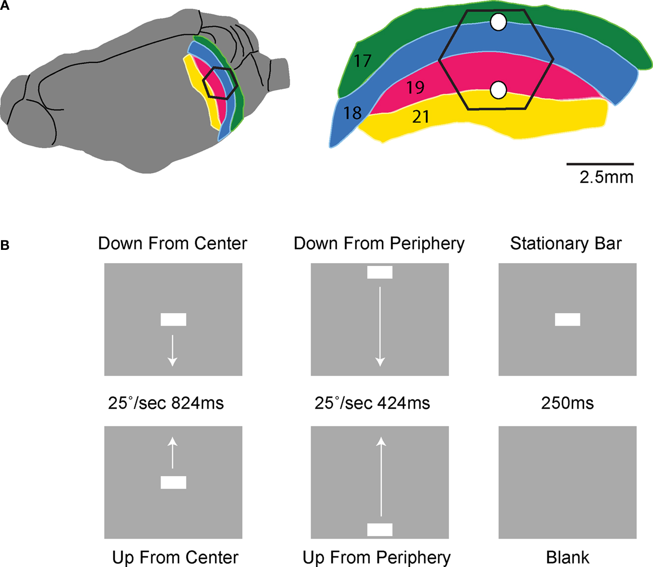
Figure 1. Experimental conditions and ferret visual areas. (A) The left hemisphere of the ferret brain with visual areas 17, 18, 19, and 21. The cortex monitored by the hexagonal photodiode array is delimited in black. The cytoarchitectural borders between areas 17 and 18 and between areas 19 and 21 correspond to the mapping of the vertical meridian in the FOV on the cortex. The two white dots mark the expected mappings of the CFOV. The relation between hexagon borders and cytoarchitectural borders (and hence the CFOV mapping) vary somewhat between animals. Each diode picks up a signal from a cortical spot of 150 μm in diameter. (B) The stimulus conditions. All stimulus conditions were compared to a gray screen (blank condition).
The cortex was stained for 2 h with the VSD RH1838 (0.53 mg ml−1, n = 10) or RH1691 (0.53 mg ml−1, n = 4) (Optical Imaging, Rehovot, Israel). After staining, the cortex was rinsed with artificial cerebro-spinal fluid the chamber was filled with silicon oil and sealed with a cover glass. The retinotopic site for the CFOV (right eye) was marked on the photo of the operative field. The photodiode array used to record the VSD signal was a 464-channel photodiode array (H469-IV WuTech Instruments Gaithersburg, MD, USA) fitted with a macroscope with a 5× objective (Red Shirt New Haven, CT, USA). Images were acquired at a rate of 1.6 kHz. The stimulus presentation was synchronized to the ECG (electrocardiogram) QRS signal, and respiration was stopped during stimulus presentation (2 s).
Experimental Conditions
The six experimental conditions were presented in a balanced random order on a video monitor with a refresh rate of 120 Hz located 57 cm in front of the animal. The stimulation was controlled using a VSG series IV system (Cambridge Research Systems, Kent, UK). The stimulus was a 1° × 2° horizontalbar (64.5 cd m−2) on a homogenous grey background (7.2 cd m−2). There were five stimulus conditions and one baseline condition (n = 10) (Figure 1
): (1) background (N = 14): a homogenous grey background (7.2 cd m−2) presented continuously, also between trials. (2) stationary bar (N = 14): a presentation of a stationary bar for 250 ms in the CFOV; (3) bar moving downwards from center FOV (N = 14): a bar moving downwards along the vertical meridian starting at the CFOV moving a total of 10.5° with a velocity of 25° s−1 for a period of 424 ms. The motion started immediately when the bar was displayed. (4) bar moving upwards from center FOV (N = 14): a bar displayed moving upwards along the vertical meridian with the same velocity for a period of 424 ms. (5) a downward moving bar starting in the peripheral FOV (N = 14) moving at the moment it was displayed 10.5° above the CFOV and moving vertically down along the vertical meridian for a total of 21° with a velocity of 25° s−1 for a period of 824 ms; (6) upward moving bar starting in peripheral FOV (N = 14); the bar starting moving at the moment of display 10.5° below the center of FOV and moving vertically along the vertical meridian with 25° s−1 for a period of 824 ms. As only one velocity of motion from peripheral FOV was tried in 14 animals, we included a further control in which one additional animal had the following stimulus conditions (1) upward and (2) downward moving bars starting 10.5° below and above the CFOV respectively, and moving for a total of 21° with a velocity of 12.65° s−1 for a period of 1650 ms.
Analysis of the VSD Signal
All VSD signals were analyzed in terms of fractional fluorescence, the details of which have been described elsewhere (Roland et al., 2006
; Ahmed et al., 2008
; Eriksson et al., 2008
). In brief, the signal in the blank (background alone) condition was subtracted from the signal of the stimulus conditions and divided by the fluorescence obtained with totally dark surroundings (dark screen) to yield the fractional fluorescence (ΔF/F0). Twenty to thirty subtractions were averaged and the result is referred to here as ΔV(t). Using the amplitude fluctuations in the pre-stimulus interval to define the noise level, the ΔV(t) was thresholded at p < 0.01 of being noise. In this we assumed the amplitude fluctuations to be not significantly different from a Gaussian distribution. A threshold of estimated p < 0.01 was set for each photodiode detector channel and divided by the number of channels (464) to give the Bonferroni corrected value of p < 0.01.
Two types of normalization procedures were used, normalization to the maximum ΔV(t) value in time,  and normalization the maximum ΔV(t) value in space,
  . For the spatial normalization this meant that for each frame of our VSD recordings, the diode channel with the highest ΔV(t) would be set to 1 and all other channels of that frame would be relative to that. For Figure 7 and Movie 9 in Supplementary Material a specific additional normalization scheme was used. In this procedure each diode is made relative to itself within a 25-ms sliding window, such that for each time point
  . Using this scheme we can then monitor when the activity at each diode reaches it’s maximum relative to its self, rather than relative to the surrounding diodes.
and normalization the maximum ΔV(t) value in space, . For the spatial normalization this meant that for each frame of our VSD recordings, the diode channel with the highest ΔV(t) would be set to 1 and all other channels of that frame would be relative to that. For Figure 7 and Movie 9 in Supplementary Material a specific additional normalization scheme was used. In this procedure each diode is made relative to itself within a 25-ms sliding window, such that for each time point . Using this scheme we can then monitor when the activity at each diode reaches it’s maximum relative to its self, rather than relative to the surrounding diodes.Electrophysiology
We made 64 electrode penetrations perpendicular to the cortical surface along the estimated course of the vertical meridian using a single shank 16 channel laminar probe (NeuroNexus, Ann Arbor, MI, USA). The resistances of the 16 recording sites were ∼3 MΩ. The sites were separated by 100 μm. Signals were routed through an RA16AC head stage to an RA16PA Medusa preamplifier and amplified at 40 K using the RA16 Medusa Base station (Tucker-Davis Technologies, Alachua, FL, USA). For multiunit recordings the signal was digitally band pass filtered between 100 Hz–10 kHz and for local field potential recordings between 1 Hz–10 kHz. Signals were acquired and written to a hard-drive using CED power 1401 AD-converter and Spike 2 Software (Cambridge Research Systems). All subsequent analysis was done using Matlab R13 (The MathWorks, Natrick, MA, USA). At each recording site RF’s were mapped using the m-sequence.
Mapping the multiunit responses
In order to define the retinotopic site of our stimulus during object motion we mapped the RF at each penetration site along the vertical meridian using the m sequence described above. The distances, in centimeters, between these RF centers on the monitor were then related to the cortical distance, in millimeters, separating the penetration sites from which the RF’s were taken. Since we know the time difference between the bar on the screen and the peak MUA or the max ΔV(t) at the cortical sites from which the RF’s were measured, we could then calculate the velocity with which the representation traveled along the vertical meridian specifically for each animal.
To establish the location of the different layers we estimated the current source density (CSD) from the second spatial derivative of the local field potentials, (Nicholson and Freeman, 1975
; Rappelsberger et al., 1981
), recorded from our 16 lead laminar probes. For a stationary bar there is an early “sink” in layer 4 reflecting the early input from the thalamocortical axons to the neurons in cortical layer 4, as well as “sources” in the infra and supragranular layers. These sinks and sources are visualized as in Figure 2
. The maximal sink was then used as a functional measure of the location of layer 4. The sources were used to indicate the location of the supra and infragranular layers (Mitzdorf and Singer, 1978
).
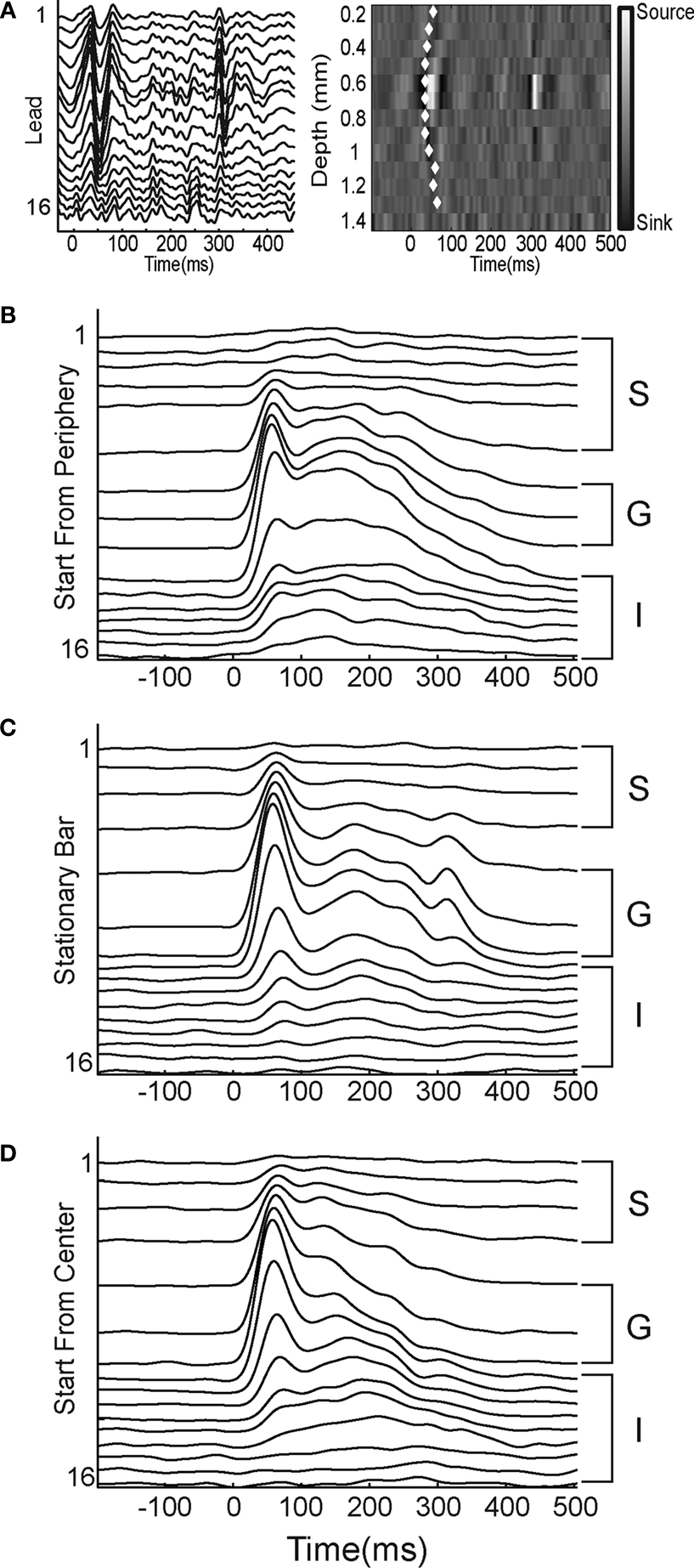
Figure 2. Laminar MUA at the retinotopic sites of the appearance of the bar. (A) Laminar local field potentials (left) and CSD (right) in response to a stationary bar presented for 250 ms at the CFOV. Note the sinks in layer IV 30–35 ms after the start of the stimulus and again at 290 ms (OFF response). The white diamonds mark the onset of statistically significant MUA on each lead (p < 0.01, see Materials and Methods). (B–D) Laminar PSTHs, average of 50 trials, filtered with a 10 ms Gaussian temporal filter. S supragranular layers, G granular layer; I infragranular layers of the moving bar starting from the peripheral FOV (B), the stationary bar (C), and the moving bar starting from the CFOV (D). Note similarities in the ON responses.
Calculating significance in the MUA
In order to calculate significant increases in the MUA, a Poisson distribution was fitted to the spike trains in the pre-stimulus period and spikes from the background trial. Spike trains passing both the criterion of having significantly increased discharge rate compared to the pre-stimulus period of p < 0.01 and increased rate compared to the background condition of p < 0.01, were considered statistically significant periods of firing.
Anatomical Verification, Cytoarchitecture, and Spatial Averages
The histological verifications, cytoarchtecture borders (Figure 1
), and the reconstruction matching the VSD and electrophysiological recordings were done as described in (Eriksson et al., 2008
). In Figure 7 and Movies 2, 4 and 7 in Supplementary Material we present the spatial means of the ΔV(t) of seven animals. To produce this figure and movies, the images of the cortex from all animals were centered to the center of gravity of the ΔV(t) at the 17/18 retinotopic site (monitored by five photodiode detectors). Subsequently the cytoarchitectural borders in the cortical images were aligned to the mean course of the cytoarchitectural borders between areas 17 and 18, and 18 and 19, and 19 and 21 by simultaneous standard affine transformations (Roland and Zilles, 1994
).
Here we first report the changes in firing rates in the supragranular (S), granular (G), and infragranular (I) cortical layers, and the changes in ΔV(t), the dye signal, in response to a stationary bar presented in the CFOV. Then we compare the laminar firing rates and ΔV(t) changes to those obtained when a moving bar is suddenly introduced in the CFOV. Finally we compare the laminar firing pattern and ΔV(t) changes from these two stimulus conditions with those obtained when the bar is introduced moving in the peripheral FOV. Whereas the MUA came from 16 locations from the pial surface to the white matter, the dye signal, ΔV(t), originates almost exclusively from the upper layers of the cortex, layers 1–3 (Kleinfeld and Delaney, 1996
; Petersen et al., 2003
).
VSD Changes and Laminar Spiking to a Stationary Bar
The bar was presented in the CFOV. This means that the bar should map on the cortex where the retinotopic map of the vertical meridian crosses the retinotopic map of the horizontal meridian. This happens at two cortical spots in our FOV, one at the 17/18 border and one at 19/21 border (Figure 1
A). Indeed the bar mapped at the 17/18 and 19/21 areal borders (Movie 1 in Supplementary Material).
We also recorded the local field potentials from all leads of the laminar probe, and from these we estimated the CSD across the laminae (Figure 2
). Independent of the histology we could then determine the functional location of the layer IV-lower layer III transition (Mitzdorf and Singer, 1978
). For a stationary bar there is an early “sink” in the G layer reflecting the early input from the thalamocortical axons as well as “sources” in the S and I layers (Figure 2
A).
After the appearance of the bar, the statistically defined onset of firing, see “Materials and Methods”, occurred first in the G layer (mean = 34 ms, SEM = 4 ms, N = 11). This was significantly, p = 0.001, earlier than the onset of firing in the S layers (mean = 53 ms, SEM = 12 ms, N = 11), as well as significantly, p = 0.01, earlier than the onset of firing in the I layers (mean = 60 ms, SEM = 11 ms, N = 11). In these and subsequent comparisons the mean MUA rate from the three leads covering the G layer was compared to the means five leads covering the S and I layers respectively. In response to the stationary bar at the cortical site representing CFOV at the 17/18 border the MUA had three clearly defined peaks. The first of these peaks, which we will refer to as the ON peak, occurred at 48.3 ms, SEM = 1.6 ms, N = 11 in S layers, at 49.6 ms, SEM = 1.2 ms, N = 11 in the G layer, and at 55 ms, SEM = 2.6, ms, N = 11, in the I layers. Not all S and I multiunits that showed significant activity in response to the presentation of the bar had this early ON component, and those that did not were excluded from the analysis of the timing of the ON peak, although they were not excluded from the analysis of the timing of response onset. Those S and I multiunits that did not have an ON peak were always those that were the furthest away from the center of the G layer, and had peak and onset times that were more closely associated with the second peak of the G layer response. The second peak occurred at 119.4 ms, SEM = 6.8 ms, N = 11 in the S layers, at 135.8 ms, SEM = 10 ms, N = 11 in the G layer and at 154 ms, SEM = 8.1 ms, N = 11 in the I layers. Finally there was a third peak corresponding to the OFF response, as reflected also in the laminar recordings (Figure 2
C).
The ΔV(t) increased at the time when the spiking became significant. The ΔV(t) at the cortical site of the bar representation had statistically defined onsets, see “Materials and Methods”, significantly (p = 0.008) earlier at the 17/18 border (mean 47 ms, SEM = 3.5 ms, N = 14) than at the 19/21 border (mean = 63 ms, SEM = 14 ms, N = 14) (Movie 1 in Supplementary Material). From the bar representation at the 17/18 border, the ΔV(t) spread laterally with an average velocity of 0.12 mm ms−1 in accordance with earlier results from cats and ferrets (Grinvald et al., 1994
; Slovin et al., 2002
; Roland et al., 2006
, Movie 1 in Supplementary Material). As a possible consequence the amplitude of the average ΔV(t) decreased only moderately by 28% of the maximal response/mm from the center of the bar representation to the cortex representing the object background, (N = 14). Starting at 65 ms an increase of the ΔV(t) from the retinotopic site of the bar in area 19/21 traveled towards the retinotopic site of the bar at the area 17/18 border. This was seen in all animals (Movie 2 in Supplementary Material). This feedback was described earlier, (Roland et al., 2006
). The time derivative of the ΔV(t), the d(ΔV(t))/dt followed the average firing rate closely with a few ms delay up to 60 ms (data not shown; see also Eriksson et al., 2008
).
Population Membrane Potential Changes and Laminar Spiking to a Bar Introduced Moving from the Center of Field of View
Dynamics at the cortical point of CFOV
When a bar is presented moving along the vertical meridian of the FOV there should be one bar representation moving along the cytoarchitectural borders between visual areas 17 and 18 and another representation of the bar moving along the border between areas 19 and 21 (Figure 1
A). Indeed that was the case (Movies 3 and 4 in Supplementary Material).
In the motion conditions, the luminance bar moved with constant velocity of 25° s−1 up or down the vertical meridian of the FOV. Just like the stationary bar, the bar introduced moving from the CFOV elicited an ON response at the cortical site representing the CFOV (Figure 2
D). This initial ON response was indistinguishable from the ON response evoked by the stationary bar (Figure 2
C). As for the stationary bar, the onset of significant firing occurred first in the G layer (mean = 31 ms, SEM = 2 ms, N = 11). This was significantly, p = 0.002, earlier than the onset of significant firing in the S layers (mean = 50 ms, SEM = 7 ms, N = 11) as well as significantly, p = 0.00015, earlier than the onset of firing in the I layers (mean = 55 ms, SEM = 6 ms, N = 11) (Figure 3
Top). The MUA had only two peaks, an ON response peaking at 46.5 ms, SEM = 1.5 ms, N = 11 in the S layers, at 49.2 ms, SEM = 1.5 ms, N = 11, in the G layer and at 52.8 ms, SEM = 1.2 ms, N = 11 in the I layers. The second peak occurred at 141 ms, SEM = 6.6 ms, N = 11 in the I layers at 135 ms, SEM = 6.7 ms, N = 11 in the G layer and at 142 ms, SEM = 7.6 ms, N = 11 in the I layers. For the ON response peaks there were no statistical differences in their timing between layers (p > 0.1 for comparison of S and I layers versus the G layer). Neither were there any differences between ON peaks for the stationary bar and the bar moving from the CFOV (p > 0.2 in each case). So from the laminar MUA, the ON response to the moving bar was not different from the ON response to the stationary bar at the CFOV. (Figures 2
C,D).
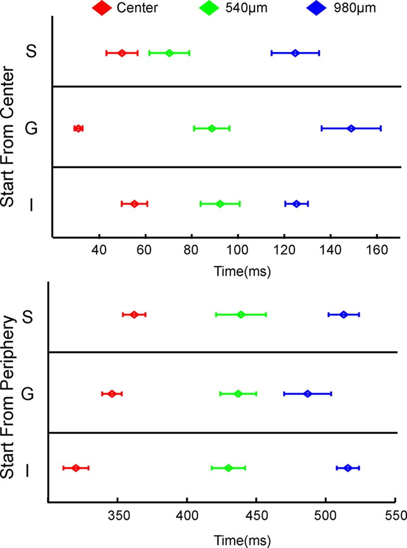
Figure 3. Statistically significant laminar onsets of MUA at three cortical sites. At each site along the 17/18 border, the statistically defined onset of firing for the five leads corresponding the supragranular (S) layers, the three leads corresponding to the granular (G) layers and the five leads corresponding to the infragranular (G) layers were pooled to give a mean S, G, and I onset for each animal. The mean and SEM for all 11 animals are shown. Note that these values were taken from both upward and downward movement conditions, i.e. the data points at 540 μm are taken from recordings 540 μm lateral to the center for upward bar motion and 540 μm medial to the center for downward bar motion.
The ΔV(t) ON-responses at the cortical points representing the CFOV however differed from ON responses to a stationary bar at the same position. First the statistical onsets were significantly earlier at both the 17/18 (p = 0.04) and the 19/21 (p = 0.02) area borders (17/18 mean onset 40 ms, SEM = 1.7 ms, N = 14; 19/21 mean onset 50 ms, SEM = 3.3 ms, N = 14). Second, while the timing of the ΔV(t) maximum at the CFOV at the 17/18 and 19/21 area borders was not significantly different between the motion and stationary conditions, the amplitude at the 19/21 border was significantly greater (p = 0.006) for the motion condition (mean = 7.3 e-4, SEM = 1.7 e-4, N = 14) than for the stationary bar condition (mean = 5.2 e-4, SEM = 1.5 e-4, N = 14), suggesting that the S 19/21 neurons might have a preference for moving objects over stationary objects. The average ΔV(t) increased first symmetrically around the representation of the CFOV at the 17/18 border and at 30 ms this increase was accompanied by a lateral spreading ΔV(t) increase, propagating with an average velocity comparable to that in the static bar condition 0.11 mm ms−1 (Movies 3 and 4 in Supplementary Material). Third, whereas the amplitude of the ΔV(t) ON response to the stationary bar was maximal at the cortical point of CFOV, the amplitude of the ΔV(t) ON response to the moving bar increased in the direction of motion. Some of these findings may be explained by the ΔV(t) dynamics at or near the cortical point of CFOV. Movie 5 in Supplementary Material shows the average difference in ΔV(t) between the bar introduced moving from the CFOV and the bar introduced stationary at the CFOV. Already at 33 ms one can see the ΔV(t) became asymmetrical with respect to the cortical representation of CFOV. Thereafter the peak of the ΔV(t) moved in the direction of object motion (Movies 4 and 5 in Supplementary Material).
Dynamics when the bar moved away from the CFOV
As the bar representation moved away from the cortical point of CFOV, the laminar firing rates transformed, from having a clear ON response to a temporal pattern with more gradual increases towards a peak and a more gradual decrease without any apparent OFF responses. First, the onsets as well as the amplitudes of the statistically significant firing changed between the laminae. At 540 μm from the retinotopic CFOV, neurons in S layers started to fire prior to the neurons in G and I layers (Figure 3
). Figure 4
shows the transformation of the laminar firing from having the highest rates at the cortical point of the CFOV in the G layer, to having the highest average rates in I layers.
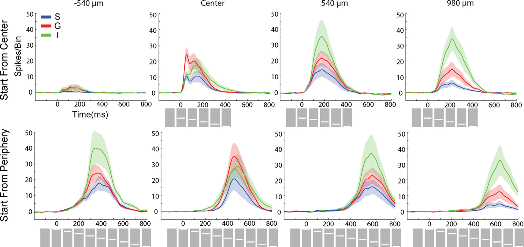
Figure 4. Average laminar MUA rates (N = 11) to the bar moving from the CFOV (Top) and the bar moving from peripheral FOV (bottom). Electrode penetrations at −540 μm (i.e. in the direction opposite to motion for bar motion beginning at the CFOV, and prior to entering the CFOV for bar motion originating in the peripheral FOV; at the retinotopic point of CFOV (center); and at 540 μm and 980 μm in the cortical direction of motion along the 17/18 border. As in Figure 3
data from both upwards and downwards movement conditions have been pooled. Blue; MUA of S layers, Red: MUA of the G layer, Green: MUA of the I layers. Mean ± SEM. Bin width: 10 ms. Grey squares with white bars indicate the position of the bar on the monitor over time.
Figure 5
shows how the ΔV(t) and its time derivative d(ΔV(t)) dt was related to the mean firing rate across all layers at each cortical position along the motion path of the cortical bar. The d(ΔV(t))/dt is related to the inward/outward current of the cells in the S layers (Eriksson et al., 2008
). At the cortical point of the CFOV, and thus at the retinotopic point where the moving bar was introduced initially, the MUA and, with a short delay, the d(ΔV(t))/dt increased and was correlated with the MUA up to 90 ms (R = 0.9, p < 0.00001). This indicated that the firing at the cortical representation of the bar at the CFOV may drive the d(ΔV(t))/dt in this time interval (see also Eriksson et al., 2008
). From Figure 5
one can see that whereas the derivative of the ΔV(t), d(ΔV(t))/dt follows the MUA at the cortical point of CFOV, the d(ΔV(t))/dt leads the average MUA at 540 μm and also later at 980 μm. The progression of the d(ΔV(t))/dt thus appeared as a fast movement of the ON transient in the cortical direction of motion in S layers (Figure 5
). From 60 ms up to 100 ms (540 μm) the layer 2–3 neurons lead the statistical onset of the MUA (Figure 3
).
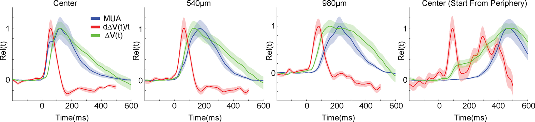
Figure 5. ΔV(t), d(ΔV(t))/dt and MUA of the moving bar. The MUA was first averaged across all 16 leads of the laminar probe, and then averaged across all animals to give the mean MUA for each cortical location. The ΔV(t) and the d(ΔV(t)/dt at each electrode penetration site for each animal were similarly averaged to give the mean ΔV(t) and the mean d(ΔV(t))/dt. These values were then normalized in time to give the mean MUA rel(t), mean ΔV(t)rel(t) and mean d(ΔV(t))/dt rel(t), see also “Materials and Methods”. Again data from both upward and downwards movement conditions were pooled as in Figure 3
. Shaded areas indicate the SEM. At the cortical point representing the CFOV, the d(ΔV(t))/dt rel(t) (the inward current in the S layers) follows the MUA rel(t) with a lag of a few ms up to 70 ms. At 540 μm the MUA rel(t) does not appear to drive the d(ΔV(t))/dt rel(t). At 980 μm the ΔV(t) rel(t) leads the MUA rel(t) by some 200 ms. Center (Start from periphery): same variables measured for the bar starting in the peripheral FOV at the retinotopic point of CFOV.
Later on, at 200 ms, the peak firing had moved 980 μm from the cortical point of CFOV. Here the rate of the MUA in the I layers is now significantly greater than that in the G and I layers (Figure 4
), and the I neurons together with layer 2–3 neurons lead the onset of MUA in G layers (Figure 3
). This indicated a further transformation of the laminar spike trains that was not initiated by the G neurons. At this cortical position at the 17/18 border, both the d(ΔV(t))/dt peak and the ΔV(t) peak lead the peak of the MUA averaged across layers (Figure 5
). Notably, only very sparse MUA was seen at 540 μm in the direction opposite to the cortical direction of motion of the bar representation (Figure 4
) and no significant MUA appeared at 980 μm in the opposite direction (data not shown).
So when an object, a moving bar, was introduced moving in the FOV, the initial firing in areas 17/18 in all cortical layers could not be distinguished from an ON response to a static bar. However the onset of the ΔV(t)) came earlier both at the 17/18 border and at the 19/21 border for a moving bar. Further the amplitude of the response at the 19/21 border was significantly greater for a moving bar than for a stationary bar. There was a strong d(ΔV(t))/dt and ΔV(t) transient propagating in the cortical direction of motion already from 40 ms. Also during the first 980 μm of cortical motion of the maximal firing, the laminar firing patterns changed radically. First the G neurons, then the S neurons, and finally the I neurons together with the S neurons lead the firing onsets only in the direction of cortical motion.
As the conditions with the bar starting at the CFOV did not provide the whole course of the bar motion over the cortex due the restricted part of cortex monitored by the photodiode array, we also included two conditions in which the bar started in the peripheral FOV.
Population Membrane Potential Changes and Laminar Spiking to a Bar Introduced Moving from the Peripheral Field of View
Feedback and mapping the cortical trajectory of the bar
In these two conditions, the moving bar was introduced 10.5° either above or below the CFOV (Figure 1
B). Again, the bar mapped as moving peaks of ΔV(t) along the 17/18 border and along the 19/21 border. The initial ON response in the laminar MUA was also in these conditions indistinguishable from that associated with the stationary bar (Figure 2
B). At increasing distance from the cortical starting point in the direction of cortical bar motion, first the S neurons lead the statistical onset of the firing, then the S and I neurons lead the firing (data not shown). As in the condition with bar starting at the CFOV another ΔV(t) increase moved over the cortex roughly following the cytoarchitectural border between areas 19 and 21.
At 120 ms after the start of the moving stimulus there was a ΔV(t) increase connecting area 19 with the moving maximal increase in area 17/18 and at the same time a slender increase appeared ahead of the 19/21 cortical bar representation (Figure 6
). Simultaneously an increase in the time derivative of the VSD signal, the d(ΔV(t))/dt moved from the area 19/21 border towards the 17/18 border where the d(ΔV(t))/dt increased at a point far ahead of the 17/18 moving bar representation and at the medial edge of the representation itself (Movie 6 in Supplementary Material) (increase in d(ΔV(t))/dt indicates increased inward current or “excitation”; Eriksson et al., 2008
, Figures 7
A,B). We refer to this as a feedback depolarization, because it originated in a higher order visual area and traveled towards the border of the lower order visual areas 17/18 (Roland et al., 2006
). The course of this feedback traveling over the cortex may seem strange, but may be explained by the retinotopic organization of the ferret visual areas, (Manger et al., 2002
) see “Discussion”. The feedback in the ΔV(t)rel began at 141 ms after stimulus onset (SEM = 11 ms, n = 12), traveled towards the 17/18 border with an average velocity of 0.12 mm ms−1 where it arrived at 165 ms (SEM = 11 ms, N = 12).
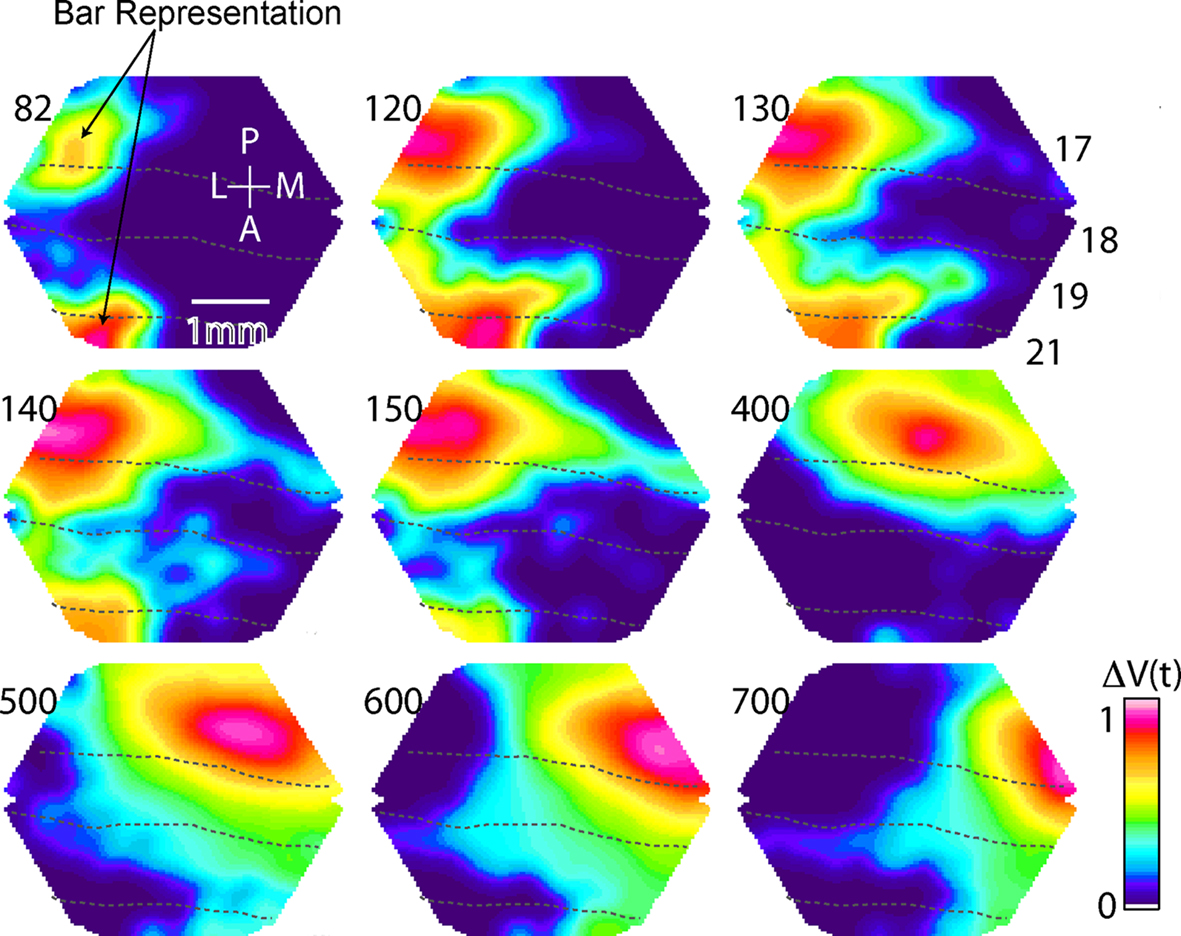
Figure 6. Summary of main VSD signal findings. Bonferoni corrected and normalized, ΔV(t)rel(s), evoked by the presentation of a bar moving downwards from the peripheral FOV in an individual animal. At 82 ms the representation of the bar is appearing at the 17/18 and 19/21 borders (dashed lines). Note that the bar mapping on the cortex only corresponds to the maximal ΔV(t) increase. At ∼120 ms a ΔV(t) increase emerges in the area between the representation at the 19/21 border and the representation at the 17/18 border and another emerges in front of the bar map in 19/21. At 140 ms this shifts direction towards the 17/18 border. Then a ΔV(t) increase emerges from the 17/18 bar map ahead in the direction of motion over cortex along the 17/18 border. This is the SRP. From 400 to 700 ms the object representation is shown as it moves regularly along the 17/18 border and arrives at the site of the tip of the SRP at ∼700 ms.
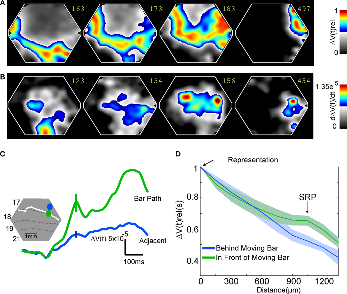
Figure 7. Feedback, and SRP. (A) The mean ΔV(t)rel for all animals exposed to the bar moving downwards from the peripheral FOV. The ΔV(t)rel (see also Materials and Methods) gives the phase information of the ΔV(t) changes over cortex. A SRP is formed along the 19/21 border as a ΔV(t)rel increase moving as a feedback towards the bar representation in 17/18 and to a point at the 17/18 border approximately 6° ahead of the 17/18 bar representation. (B) The d(ΔV(t))/dt averaged across animals exposed to the bar moving down from the peripheral FOV. Note the d(ΔV(t))/dt increase (inward current) as a feedback moving from 19/21 to the 17/18 border forming an SRP targeting a point approximately 6° ahead of the 17/18 bar representation. (C) The SRP is spatially restricted to the cortical path of the bar. The bar path was calculated for all animals by following the moving peak of the ΔV(t)rel(s). The solid white line (inset) represents an individual example. The solid green line shows the mean ΔV(t) signal for all animals from areas 17/18 within the motion path (individual example, green oval, inset). The solid blue line shows the mean ΔV(t) for all animals from areas directly adjacent to the motion path (individual example, blue oval, inset). Error bars indicate SEM at the time of the peak of the SRP. (D) The mean ΔV(t)rel(s) for all animals taken at the time of the SRP at 10 equidistant points behind, (blue line) and in front (green line) of the bar representation. The 10 points were part of the cortical motion path at or very close to the 17/18 cytoarchitectural border. To calculate the activity occurring behind the motion path (blue line), we used the two conditions in which the bar moved from CFOV. To calculate the activity in front of the motion path (green line), we the two conditions in which the bar moved from the peripheral FOV, The ΔV(t)rel(s) signal behind the moving object decays monotonically with distance. The ΔV(t)rel(s) signal in front of the moving bar shows an increase at 0.96–1.28 mm ahead of the object representation (SRP).
At 140–150 ms at the time when the feedback arrived at the 17/18 border, there was a similar, but longer, slender increase in the relative population membrane potentials ahead of the maximal increase of ΔV(t) along the area 17/18 border. As seen from Figure 6
, from 150 to 700 ms the maximal ΔV(t) increase indeed followed this path. This transient ΔV(t) increase appeared in all animals in the time interval 130–200 ms (N = 14, p < 0.01 after Bonferroni correction), but only in the direction of cortical motion of the bar (Figure 7
D). Also in all animals the path of the maximal ΔV(t) over the cortex followed the path of this directional pre-depolarization (data not shown). For this reason we called this a spatially restricted pre-depolarization (SRP). The SRP typically started some 8–10° ahead of the position of the bar representation on the cortex and then depolarized the space in between following the curvature of the cytoarchitectural border between area 17 and 18. The SRP had a well defined shape, its amplitude being significantly stronger in the motion path (mean = 1.6 × 10⁻⁴, SEM = 2.9 × 10⁻⁵) than adjacent to the motion path (mean = 5.92 × 10⁻⁵, SEM = 1.01 × 10⁻⁵, p = 0.003, two tailed t-test) (Figure 7
C). The dynamics of the SRP are best seen in Movies 6–8 in Supplementary Material, when the bar moved upwards the SRP was directed laterally over the cortex, when the bar moved downwards, the SRP was directed medially. In one animal we examined the appearance of the SRP when the bar was moving from the peripheral FOV with half the velocity i.e. 12.7° s−1. The SRP appeared for both upward as well as downward motion at 181 ± 36 ms after the start of the stimulus. At 385 ms (SEM = 30 ms, N = 12), or 8° later than the maximal statistical extent (p < 0.01) of the SRP, the bar representation moved over the point indicated by the tip of the SRP.
In 14 separate penetrations in 8 animals we recorded significant (p < 0.01) increases of the MUA at the site associated with the strong ΔV(t)rel and dΔV(t)/dt (Figures 7
A,B). To further examine the mechanisms generating the SRP, i.e. generating the relative increase in the population membrane potentials in cortical layers 1–3, we analyzed the onset of this firing in relation to the onset of the SRP. This revealed that the SRP started on average 30 ms prior to the statistically significant onset of the firing (p < 0.05; t-test two tailed, N = 12). This firing was typically not in the S layers (N = 2), but rather in the I layers (N = 12). We recorded no responses corresponding to the arrival of the SRP at this site in G layers.
Changes in the laminar MUA after the feedback
During the further course of the moving representation of the bar over the cortex, the onset of the I MUA lead the onset of the MUA in the G neurons. At the retinotopic point −540 μm, the I MUA exceeded the amplitudes of the G and S MUA (Figure 4
, lower panels). At the representation site of the CFOV, more than 2000 μm from the first cortical response to the moving bar, the onset of firing in the I neurons lead the onset of firing in G neurons by 25 ms in the whole population of animals, SEM = 14.9 ms, N = 11 (t-test; p < 0.01), Figure 3
Bottom. At this location the statistical onsets of the MUA preceded the peak MUA by 110–150 ms.
As the bar approached the CFOV, the amplitudes of the laminar MUA changed again, with proportionately more firing in the G layer. At the site representing the CFOV the mean MUA across animals peaked in the S layer at 477 ms, SEM = 7 ms, N = 11 in the G layer at 468 ms, SEM = 7 ms, N = 11 and in the I layers at 469 ms, SEM = 7 ms, N = 11, i.e. on average 58 ms delayed in relation to the time when the bar arrived at CFOV (413 ms). There was no difference in the timing of the peak MUA in the different laminae at this cortical point. At the cortical point 540 μm further on, the order of statistical onsets of the MUA changed again such that there were no differences in the order of firing between the layers (Figure 3
Bottom). And further ahead in the cortical direction of motion again the G layers trended towards leading the onsets of laminar MUA, though these differences were not significant (Figure 3
). Surprisingly, the laminar rates of firing also switched after the bar had passed the CFOV, such that the firing in I layers again became dominant and after a while at the position 980 μm from the cortical point of CFOV became statistically stronger than the firing in the G layer, which in turn was statistically stronger than was the firing in the S layers (Figure 4
Bottom).
The relation between the moving MUA maximum and the moving ΔV(t) maximum changed in a manner similar to the condition in which the bar was introduced in the CFOV. Initially the ON response and the d(ΔV(t))/dt appeared almost simultaneously, but then the ΔV(t) maximum moved in front of the MUA maximum. However when the PSTHs after the first 150 ms became more extended over time, the peak MUA approached the peak ΔV(t). At the cortical position representing the CFOV at the area 17/18 border, the timing of the two peaks did not differ significantly in space and time (Figure 5
).
During the first 170 ms, the ΔV(t) maximum also moved along the 19/21 cytoarchitectural border. However as apparent form the Movies 3–8 in Supplementary Material, the progressions of the bar maps in 19/21 and 17/18 did not initially seem to be in phase. We therefore computed the ΔV(t)rel (see Materials and Methods), averaged across all animals, to visualize the phase relations in the ΔV(t). This revealed that the phase differences in areas 17, 18, 19, and 21 gradually diminished from 200 ms to 345 ms, and after 345 ms the ΔV(t) increases were in phase. This is seen in the phase Movie 9 in Supplementary Material of the ΔV(t)rel showing that the ΔV(t) from 19/21 to 17/18 was in phase until 700 ms.
The Relation Between the Firing, Relative Membrane Potentials and Veridical Motion of the Bar
During the first 200 ms there was a spatiotemporal inconsistency between the motion of the relative membrane potential increase, ΔV(t) and the MUA averaged across layers, Figures 5 and 8
. This raises the following questions: Which physiological parameter(s) actually map the moving bar in the cortex? How is the veridical velocity of the bar related to the velocity of the cortical map of the moving bar? Is the bar mapped with a delay by the visual areas or is there some compensation for the time the signals take to travel from the photoreceptors to the cortex?
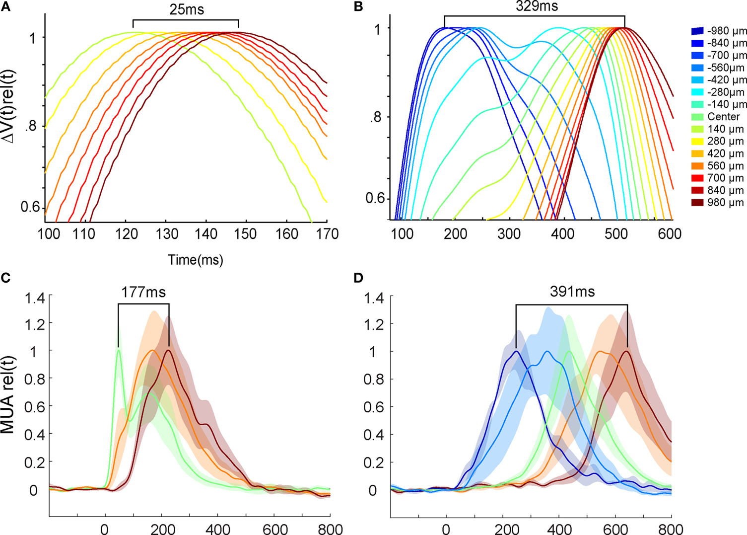
Figure 8. Peak velocities of VSD signal and MUA. Top: The mean ΔV(t) rel(t) signal from all animals taken from 15 locations at the 17/18 border and along the path of the moving object representation. Again upwards and downwards movement conditions have been pooled. (A) For a bar moving from CFOV the peaks move with a mean velocity of 0.039 mm ms−1 in the time interval shown. (B) For a bar moving from the peripheral FOV the peak activity propagates over cortex with a mean velocity of 0.005 mm ms−1. Bottom: The mean MUA rel(t) averaged over the 16 leads of the laminar probe for all animals at five sites along the path of the moving object representation on the 17/18 areal border. Downwards and upwards movement conditions are pooled. Color scale is the same as top. (C) Bar moving from CFOV. The peak MUA moves with an average velocity of 0.0055 mm ms−1 for the first 980 μm. (D) Bar moving from peripheral FOV. The peak MUA moves with an average velocity of 0.005 mm ms−1.
When the bar was introduced moving at the CFOV, the ΔV(t)rel(t) maximum traveled with a mean velocity of 0.039 mm ms−1 (SEM = 0.0164 mm ms−1, N = 20) over the cortex out from the cortical point representing the CFOV (Figure 8
A). This was slower than the lateral spreading depolarization (0.12 mm ms−1), but much faster than the bar velocity in the FOV (25° s−1). If one assumes that each mm of cortex represents 5° of visual angle (Manger et al., 2002
), this moving peak traveled at 200° s−1. When the bar was introduced moving in the peripheral FOV averaged over the first 1.96 mm the mean ΔV(t)rel maximum traveled with a velocity of 0.0059 mm ms−1, Figure 8
B. Under the same assumption this would correspond to 29° s−1. Along the border between area 19 and 21 the local ΔV(t)rel maximum moved along from 180 ms and onwards with an average velocity of 0.0049 mm ms−1 (SEM = 0.00049 mm ms−1, N = 14), but the start of this cortical motion was not monitored in all animals as this was outside the recording area of the photodiode array.
When the bar was introduced in the CFOV, the mean peak MUA moved over the first mm of cortex with an average velocity of 0.0055 mm ms−1 (SEM = 0.0007 mm ms−1, N = 10) giving an estimated velocity of 27.7° s−1 (Figure 8
C). The peak MUA from all animals, recorded in response to a downward moving bar originating in the peripheral FOV, traveled with a velocity of 0.005 mm ms−1, (SEM = 0.00050 mm ms−1, N = 14) over the cortex (Figure 8
D). This would correspond to a velocity in the FOV of 25° s−1, again assuming that 5° along the vertical meridian mapped as 1 mm of cortex. From this the motion of the averaged MUA peak across layers seemed a good estimate of the veridical bar motion.
When introduced in the FOV the ON responses to the bar peaked at 52 ms (not significantly different from the stationary bar). Under the assumption that the MUA peak mapped the initial position of the bar this gave a delay of 52 ms in the cortical mapping. When the bar passed the cortical point of CFOV the G layer MUA peaked at 469 ms (with no significant difference between the G, I, and S layers (Figure 4
). As the bar reached the CFOV at 413 ms this gave a delay in mapping of 58 ms.
When a moving object was introduced in the visual FOV, the cortical dynamics of the laminar firing rates and the VSD signal went through several phases.
• At the cortical point, corresponding in retinotopy to the point in the visual field where the bar was introduced, it was mapped like a stationary object with an ON response starting in the G layer and then in S and I layers, followed by a lateral spreading in the VSD signal.
• At 40 ms, the VSD signal deviated from this position and moved in the cortical direction of motion and at 64 ms the neurons more than 500 μm away started to fire in S layers (i.e. the S layers now preceded the G and I layers).
• At 120 ms the neurons in areas 19/21 computed a SRP in the cortical direction of motion. This was immediately followed by a feedback signal to the area 17/18 border far ahead of the bar representation there.
• A similar SRP then appeared at the 17/18 areal border, and this was followed some 30 ms later by the firing of multiunits primarily in the I layers but also in the S layers.
• Following these events, the statistical onsets of the firing lead the peak firing by some 100–150 ms along the cortical path of motion.
• From 300 ms the peak of the MUA and the peak of the ΔV(t) moved along the 17/18 border synchronously. Subsequently the ΔV(t) in areas 19/21 and 17/18, which previously had been out of phase, started to move along the direction of movement in phase.
• When the bar representation at the 17/18 border passed the cortical domain for CFOV, the G layer firing was again dominant.
• After passing the CFOV this relationship again changed with the amplitude of firing in the I layers eventually again surpassing the amplitude of firing in both the S and G layers.
Changes in the VSD signal, ΔV(t), in vivo reliably reflect changes in the membrane potentials of the cells in the S layers of the cortex, (Petersen et al., 2003
; Ferezou et al., 2006
; Berger et al., 2007
; Eriksson et al., 2008
). So our interpretation of increases in ΔV(t) are increases in the S population membrane signal. Our interpretation of ΔV(t) decreases are decreases in the S population membrane potentials. As the derivative d(ΔV(t))/dt is related to the inward current in the S population of cells (Eriksson et al., 2008
), we interpret increases in d(ΔV(t))/dt as increases in the inward current and decreases as decreases of the inward current.
The Stationary Phase
No matter whether the bar was introduced moving at the CFOV or the peripheral FOV it was initially mapped at the corresponding retinotopic point in cortex as a stationary bar with an ON response in the MUA. Judging from the relation between the MUA and the d(ΔV(t))/dt (Figure 5
), the MUA was likely to drive the increases in the membrane potentials along the 17/18 border.
It makes ecological sense that novel objects entering the FOV will elicit a strong cortical response. As this appears in an anesthetized animal, it is not dependent on any conscious attention mechanism. Rather it is a computation by the afferent visual system and the early cortical areas that secure saliency of suddenly appearing objects in the visual scene. Already at the adjacent point, 540 μm, the peak MUA comes considerably later and the shape of the PSTH changes from the stationary object pattern with a sharp ON response to a more slowly increasing and decreasing PSTH (Figure 4
).
The Supragranular Phase
This phase started with a moving increase in the population membrane potential in layers 1–3 in the direction of cortical motion of the bar. Judging from the shape of the d(ΔV(t))/dt resembling the ON response at cortical positions up to 980 μm from the starting point of cortical motion of the bar, the neurons at the starting point could have driven this moving inward current increase. From 64 ms, approximately when the d(ΔV(t))/dt was near maximal, the S neurons started to fire up to 540 μm from the starting point. Notably, this excitation appeared only in the direction of cortical motion. In our data there was no support for the alternative that this excitation was secondary to G layer firing, because the onset of significant firing in the G layer came significantly later (Figure 3
). Also the alternative that this excitation was the consequence of feedback from higher order areas may be less likely as the firing then would be supposed to start in both S and I layers, (Felleman and Van Essen, 1991
; Series et al., 2003
; Sillito et al., 2006
) and see below. During this period, the peak firing rate of the neurons across all layers moved with a cortical velocity of 0.005 mm ms−1, that corresponded to the bar motion in the FOV.
Feedback and SRP, the Supragranular and Infragranular Phase
The ferret has, as other carnivores, feedback axons from areas with motion sensitive neurons as well as from areas 19 and 21 to area 17 and 18, (Cantone et al., 2005
, 2006
; Payne and Lomber, 2003
; Grant and Hilgetag, 2005
; Sillito et al., 2006
). As the increases in the laminar firing rates in this phase seemed primarily to engage S and I layers they might be induced by feedback from higher order areas known to target S and I layers, but not the G layer. Support for this came from the results that the increase in d(ΔV(t))/dt indeed moved at 111–135 ms from the 19/21 border to target the 17/18 border in the S layers (Figure 7
; Movie 6 in Supplementary Material) and that the maximum ΔV(t)rel also moved from the 19/21 border in the interval 150–180 ms (Figure 7
). Furthermore at 980 μm from the CFOV, the significant S and I MUA started at 124 and 125 ms respectively (Figure 3
).
The SRP in area 17/18 was invariably preceded by a feedback from areas 21 and 19 and it disappeared at 200 ms, although the retinal input continued (Movies 7 and 8 in Supplementary Material). This made the SRP unlikely to be of retinal origin. In the condition in which the bar started from the CFOV, there was also a feedback apparent in the average ΔV(t)rel across animals (data not shown), but the SRP was hidden from measurement due to the restricted cortical area imaged by the photodiode array. The ferret cortex, as the cortex other carnivores and of primates has a larger representation of the center of the visual field along the vertical meridian, compared to the horizontal meridian (White et al., 1999
; Manger et al., 2002
). This anisotropy can be seen in the mapping of a stationary square stimulus in the CFOV (Roland et al., 2006
). The effect is small at most 1–1.5°, and not comparable to the extent of the SRP. Furthermore, the anisotropy goes in both directions, up and down, but the SRP only appeared in the direction of motion (Figure 7
). Also the SRP appeared transiently whereas the anisotropy should be continuously represented. The firing in S and I layers in this phase may be related to the feedback and formation of the SRP’s (Movies 6–8 in Supplementary Material).
Progress in Phase, All Laminae Showing Premature Firing
As shown in Movie 9 in Supplementary Material, which was the only result providing the evidence for the in phase progression of the membrane potential changes in the S layers, the ΔV(t) peaks started to progress over the cortex in phase and with a velocity in retinotopic coordinates corresponding to the velocity of the bar motion in the FOV (Figure 5
, start from periphery). There could be several mechanisms governing the phase coherence between areas 21, 19, 18 and 17. However, with the possible exception of fast reciprocal communication between these areas, (feed-forward/feedback), our results are insufficient to distinguish between the alternatives. Speculatively, a slightly earlier firing by the 19/21 neurons, perhaps because of their larger RF could, combined with feedback, also provide phase coupling, as could a common thalamic or other input to areas 21, 19, 18, and 17, (Payne and Lomber, 2003
; Sillito et al., 2006
).
Between 180 and 400 ms, the laminar firing pattern switched from S neurons and I neurons leading the statistical onset of the MUA to all laminae firing equally in advance of the peak firing rate (Figures 3 and 4
). The laminar pattern of firing now changed to a triangular spike train profile. That the time to peak firing for moving objects is increased compared to stationary stimuli has been noted earlier (Motter and Mountcastle, 1981
; Andersen, 1997
; Merchant et al., 2003
). From our data, the increase in the latency between onset and peak firing was related to onsets in firing in all layers that occurred long before the cortical mapping of the bar was expected to take place according to the veridical velocity of the bar motion.
In interpreting these changes in laminar MUA, one main alternative is that peripheral and central vision of object motion in areas 17/18 is organized differently, (Orban et al., 1975
; Azzopardi and Cowey, 1993
). This is supported by our result that the MUA in the G layer dominated and might have been driving when the object was passing the CFOV and I MUA dominated and might have been driving when the object moved in the peripheral FOV (Figures 3 and 4
). This hypothesis however cannot account for the findings that the laminar ON responses were identical in CFOV and peripheral FOV. Neither can this hypothesis explain that the G layer MUA was leading the onset of firing at later stages (Figure 3
). Furthermore it does not explain the dynamics of the membrane potentials in the S layers, including the fast directional excitation (Figure 5
), the SRP (Figure 6 and Movies 6–8 in Supplementary Material), and the observed SRP and feedback from areas 19/21 (Figures 6 and 7
; Movies 6–9 in Supplementary Material).
Fixed Retina and Moving Objects, an Artificial Situation
Maintaining fixation towards one point in the FOV when a moving object enters the FOV happens, but is not the usual situation. Normally any object entering the FOV will elicit a catch-up saccade and thereafter a smooth visual pursuit that will keep the object stable on the fovea of the retina. In the human visual world most objects enter the FOV laterally, more seldom vertically. We examined only object motion along the vertical meridian in the FOV. This was to avoid the retinotopic discontinuities in the ferret areas 17, 18 and 19 (Manger et al., 2002
; Cantone et al., 2005
). For these reasons we cannot claim that our results will generalize to all directions and velocities. It is unlikely, however, that changes in direction of movement and movement velocity will affect the order in the evolving dynamics of the membrane potentials and laminar firing.
The firing in I layers and to some extent also S layers of the cortex associated with the SRP was, albeit statistically significant, much earlier and more moderate than the peak firing associated with the representation of the bar itself. This demonstrates that the brain still keeps the information about the actual object trajectory and position at the same time as it computes the SRP. Our ability to generalize our finding of the SRP to all directions is limited. The control experiment with the bar moving in two directions with half the velocity, indicate that the SRP may be present for object motion with velocities ranging from 12.7° s−1 to 25.4° s−1. Our data indicate that the SRP may first be computed in areas 19/21 with a subsequent SRP then appearing in areas 17/18. Because our FOV was limited to only four visual areas, we cannot exclude that the computation of SRP’s could start in higher order motion sensitive areas. Layer 5/6 complex cells have large RF’s (Palmer and Rosenquist, 1974
; Gilbert, 1977
). One may therefore question whether the firing of the I neurons in association with the SRP could be a consequence of the bar entering such large RF’s. This we cannot exclude, but then it is strange that this I firing appeared after a delay of 125 ms. Furthermore the SRP was well confined to the path eventually taken by the moving representation and the I firing was only in the direction of cortical bar motion. This is inconsistent with a non-specific activation of cells having a larger RF. As the vast majority of area 17 neurons projecting to superior colliculus are located in layer 5, (Palmer and Rosenquist, 1974
), the premature firing of these neurons could provide a signal for a catch-up saccade. The saccades elicited after an object moves into the FOV occur usually with latencies of 120–150 ms, (Lisberger et al., 1987
; de Brouwer et al., 2001
). This interval corresponds well with the latency at which the I neurons started to fire ahead along the 17/18 border in the direction of motion. Also during an actual saccade there is a transient excitation over cortex corresponding to the saccadic trajectory, (Slovin et al., 2002
).
Mapping of Moving Objects by Changes in Membrane Potentials and Laminar Firing
We did not do any spike sorting of the MUA, nor did we attempt to test directional sensitivity in the spike trains. We cannot therefore exclude that the fast moving excitation in the direction of motion in the S phase could have been a product of directionally sensitive populations in layer III. The laminar MUA and the VSD signal show population averages of the spiking activity and changes in membrane potentials with no preference of specific feature computations.
Given the very early significant firing in all layers a long time in advance of the mapping of the moving object in cortex in retinotopic coordinates as the peak firing rate, one may also question whether spatiotemporal RF models and energy models will be of relevance for the mapping of moving objects, (Nakayama, 1985
; Heeger, 1987
; Albright and Stoner, 1995
; Carandini et al., 1997
; Mante and Carandini, 2005
). On the other hand, if the actual mapping of the moving object in cortex is only by the peak firing rate (see below), modified spatiotemporal RF models and modified energy models could capture this aspect. However, feed-forward models cannot capture all aspects of an objects motion, especially not the computations leading to feedback communication and coherent motion mapping across cortical areas.
As soon as the bar left the retinotopic point of the CFOV the peak of the ΔV(t) was leading the peak MUA. This implied a discrepancy in space and time between the absolute VSD signal, ΔV(t), and the laminar MUA. One reason was the lateral spreading depolarization making a diffuse ΔV(t) increase much larger than the cortical retinotopic space associated with a small 1° × 2° bar. This lateral spreading depolarization is well known for stationary objects and moving gratings restricted to a part of the FOV, (Grinvald et al., 1994
; Slovin et al., 2002
; Roland et al., 2006
; Ahmed et al., 2008
; Eriksson et al., 2008
). Another reason was the fast directional excitation of the S layers presumably also responsible for the early firing in layers 2–3 (Figures 3 and 5
). This also brought the laminar firing of the G layer neurons (taking the input from LGN) out of phase with the output neurons in layer 3 of area 17/18 (sending the output to areas 19 and 21). In the S and I phase, the firing in the G layer starts to appear earlier. The spatial distribution of the significant firing in any of the six layers occupied a much larger space of the cortex than expected by a small 1° × 2° stimulus due to this premature firing in all layers. For this reason the peak MUA would be better suited to map the bar. As the location and motion velocity of the peak firing in the MUA in all layers from 70 ms and onwards was in agreement with a retinotopic mapping of the bar with a delay, the peak firing could map the moving bar.
The authors declare that the research was conducted in the absence of any commercial or financial relationships that could be construed as a potential conflict of interest.
This work was supported by a EU grant ISI 2006 027198 Decisions in Motion, and a grant from the Wallenberg Foundation to P.E.R.
The Supplementary Material for this article can be found online at http://www.frontiersin.org/systemsneuroscience/paper/10.3389/neuro.06/007.2009/
Berger, T., Borgdorff, A., Crochet, S., Neubauer, F. B., Lefort, S., Fauvet, B., Ferezou, I., Carleton, A., Luscher, H. R., and Petersen, C. C. (2007). Combined voltage and calcium epifluorescence imaging in vitro and in vivo reveals subthreshold and suprathreshold dynamics of mouse barrel cortex. J. Neurophysiol. 97, 3751–3762.
Manger, P. R., Kiper, D., Masiello, I., Murillo, L., Tettoni, L., Hunyadi, Z., and Innocenti, G. M. (2002). The representation of the visual field in three extrastriate areas of the ferret (Mustela putorius) and the relationship of retinotopy and field boundaries to callosal connectivity. Cereb. Cortex 12, 423–437.