Weill Cornell Medical College, New York, NY, USA
The interconnected areas of the visual system work together to find object boundaries in visual scenes. Primary visual cortex (V1) mainly extracts oriented luminance boundaries, while secondary visual cortex (V2) also detects boundaries defined by differences in texture. How the outputs of V1 neurons are combined to allow for the extraction of these more complex boundaries in V2 is as of yet unclear. To address this question, we probed the processing of orientation signals in single neurons in V1 and V2, focusing on response dynamics of neurons to patches of oriented gratings and to combinations of gratings in neighboring patches and sequential time frames. We found two kinds of response dynamics in V2, both of which were different from those of V1 neurons. While V1 neurons in general preferred one orientation, one subpopulation of V2 neurons (“transient”) showed a temporally dynamic preference, resulting in a preference for changes in orientation. The second subpopulation of V2 neurons (“sustained”) responded similarly to V1 neurons, but with a delay. The dynamics of nonlinear responses to combinations of gratings reinforced these distinctions: the dynamics enhanced the preference of V1 neurons for continuous orientations and the preference of V2 transient neurons for discontinuous ones. We propose that transient neurons in V2 perform a differentiation operation on the V1 input, both spatially and temporally, while the sustained neurons perform an integration operation. We show that a simple feedforward network with delayed inhibition can account for the temporal but not for the spatial differentiation operation.
A fundamental step in analyzing visual scenes is to find object boundaries. In natural images, some boundaries are defined by luminance differences; others are defined by texture differences. Most neurons in primary visual cortex (V1) are well-driven by luminance boundaries at the appropriate orientation (Hubel and Wiesel, 1959
, 1968
). Boundaries defined by differences in texture, however, are more effective stimuli for neurons in the secondary visual cortex (V2) (von der Heydt et al., 1984
, 2000
; von der Heydt and Peterhans, 1989
; Grosof et al., 1993
; Leventhal et al., 1998
; Marcar et al., 2000
; Marcus and Van Essen, 2002
; Song and Baker, 2007
). Since the larger receptive fields of V2 are produced by combining the output of V1 neurons (Foster et al., 1985
; Levitt et al., 1994
; Smith et al., 2007
), the extraction of texture boundaries by V2 receptive fields must involve computations on its V1 inputs across space. These computations must accomplish a specific goal – extraction of texture boundaries – while preserving the luminance-boundary information already extracted by V1. Thus, the extraction of boundaries from the retinal image serves as an excellent model to reveal how cortical areas interact to carry out sensory processing.
To analyze these computations, we developed a technique that focuses on the dynamics and nonlinearities underlying the extraction of texture boundaries. In particular, we measured the responses to individual grating patches (preference for one orientation vs. the other) along with their pairwise interactions (preference for orientation continuity vs. discontinuity). Importantly, because the retinal image under normal viewing conditions is not static, we designed the approach so that it could resolve interactions across both space and time.
Our analysis revealed two distinct neural subpopulations within V2. Each had responses that differed qualitatively from those in V1, but in a complementary manner. These complementary differences encompassed temporal properties, spatial properties, and prominence of nonlinearity. In broad terms, one subpopulation in V2 mainly integrates orientation signals over space and time, while the other subpopulation calculates a derivative, also both in space and time. Integration allows the subpopulation to respond to regions of uniform orientation; differentiation allows the other subpopulation to respond to boundaries, i.e. changes over space or time. Finally, we discuss to what extent simple feedforward combinations of the signals available in the V1 output can account for the observed V2 responses.
Physiological Preparation
Standard acute preparation techniques were used for electrophysiological recordings from single units in the primary visual cortex (V1) and secondary visual cortex (V2) of the primate (cynomolgus monkeys, Macaca fascicularis). All procedures were in accordance with institutional and National Institutes of Health guidelines for the care and experimental use of animals and under an approved protocol from the Weill Cornell Medical College Institutional Animal Care and Use Committee.
Experiments were performed on seven adult animals, weighing 2.5–10 kg. The preparation was similar to what was previously described (Mechler et al., 2002
; Victor et al., 2006
), and is summarized here. After an overnight fast, animals were premedicated with atropine (0.05 mg/kg, i.m.; Henry Schein, Melville, NY) and then anesthetized with ketamine (10 mg/kg, i.m.; Ketaset, Fort Dodge, IA) or Telazol (4 mg/kg, i.m.; Fort Dodge, IA) and xylazine (0.5 mg/kg, i.m.; Rompun, Bayer, Shawnee Mission, KS). Under anesthesia with isoflurane (1–2%; Hospira, Lake Forest, IL) during the surgery, an endotracheal tube was placed and catheters put in both femoral veins, one femoral artery, and the urethra. During recording, anesthesia was maintained with propofol (2–10 mg/kg h, i.v.; PropoFlo, Abbott, IL, USA) and sufentanil (1–5 μg/kg/h, i.v.; Sufenta, Janssen, Titusville, NJ), and neuromuscular blockade was induced (after all surgical procedures) and maintained with vecuronium bromide (0.25 mg/kg intravenous, i.v. bolus, 0.25 mg/kg/h, i.v.; Bedford Laboratories, Ohio). Heart rate and rhythm, arterial blood pressure, body temperature, end-expiratory pCO2, urine output, and EEG were monitored during the course of the experiment. Animal maintenance included intravenous fluids (lactated Ringer solution with 5% glucose, 2–4 cm3/kg/h), administration of supplemental O2 every 6 h, antibiotics (procaine penicillin G 75,000 U/kg i.m. prophylactically; King Pharmaceuticals, Bristol, TN, gentamicin 5 mg/kg i.m. daily if evidence of infection; Abbott, Illinois, USA), dexamethasone (1 mg/kg i.m. daily; AmTech, Teva Animal Health, Saint Joseph, MO), application of 0.5% bupivicaine (Marcaine; Hospira, Lake Forest, IL) to wounds, and ocular instillation of atropine (1%; Baush & Lomb, Tampa, FL) and flurbiprofen (0.03%, Ocufen, Alergan, Irvine, CA), and periodic cleaning of the contact lenses. With these measures, the preparation remained physiologically stable for 4–5 days.
Recording
After a craniotomy near P10, L15, the lunate sulcus was located and a small durotomy performed either over V1, or V2, or both. Extracellular recordings were made with three tetrodes (quartz-coated platinum–tungsten fibers; Thomas Recording, Giessen, Germany). The analog signal from each tetrode channel was amplified, filtered (0.3–6 kHz), and digitized (25 kHz). Once spiking activity from one or more units was encountered, the region of the receptive field(s) was hand-mapped and then centered on the display of a ViewSonic G225f 21-inch monitor (displaying a 1280 × 1024 raster at 100 Hz, mean luminance 47 cd/m2), at a distance of 114 cm. Control signals for the CRT display were provided by a PC-hosted system optimized for OpenGL (NVidia GeForce3 chipset) programmed in Delphi. Multiple single units were isolated by cluster analysis of spike waveforms initially performed on-line (Autocut, DataWave Technologies) then off-line (custom software). Isolation criteria included stability of principal components of spike waveforms and a 1.2-ms minimum interspike interval consistent with a physiologic refractory period. Spike times were identified to 0.1-ms precision.
Histology
After the completion of the recording, the tetrodes were moved back towards the cortical surface and at three locations bracketing the recording sites lesions were made by current passage (typically 12 μA × 6 s, electrode negative). After a waiting period of 1 h, the animal was deeply anesthetized with propofol (5–10 ml) and perfused (4% paraformaldehyde; EMS, Hatfield, PA) in phosphate-buffered saline. A block of brain tissue containing the tetrode tracks was then removed and allowed to sink in 10%, 20%, and 30% sucrose solution in 4% paraformaldehyde. Frozen sections were then cut parallel to the tetrode tracks, mounted and stained for Nissl in thionin staining solution (1%, Sigma-Aldrich, St. Louis, MO). The border between V1 and V2 was identified: the border is readily visible because of the distinct appearance of layer 4 in V1, which disappears in V2.
Visual Stimulation
The pupils were covered with gas-permeable contact lenses (Metro Optics, Houston, TX). Artificial pupils (2 mm) and corrective lenses were used to focus the stimulus on the retina. Foveae and the receptive fields of multineuron activity were mapped on a tangent board for each tetrode. Optical correction was established initially by use of an opthalmoscope and adjusted to maximize the responses of isolated single units to high spatial frequency visual stimuli.
Among the multiple spikes simultaneously recorded by each tetrode, one well-isolated spike was selected as the “target” neuron. Beginning with the parameters determined by the qualitative characterization, computer-controlled stimulation paradigms were used to characterize the target neuron quantitatively with sine gratings. Orientation tuning was determined by the mean response (F0) and the fundamental modulated response (F1) to drifting gratings at orientations spaced in steps of 11.25°, presented at a contrast c = (Lmax − Lmin)/(Lmax + Lmin) of 1.0, with spatial and temporal frequency determined by the initial assessment. Next, spatial frequency tuning was determined by responses to drifting gratings at a 16-fold range of spatial frequencies at the orientation determined by the orientation tuning run, and a temporal frequency determined by the auditory assessment. Temporal tuning was then assessed by responses to 1-, 2-, 4-, 8-, and 16-Hz drifting gratings at the optimal orientation and spatial frequency. Finally, a contrast response function was determined by responses to drifting gratings at contrasts of 0, 0.0625, 0.125, 0.25, 0.5, and 1.0, with orientation, spatial frequency, and temporal frequency determined by the previous quantitative runs. The position of the receptive field (RF) was first determined by auditory assessment of spiking activity using a laser pointer on the monitor screen displaying concentric rings around the currently selected center. After adjusting the center accordingly, the size of the classical RF (CRF) was determined from responses to a drifting grating (all parameters optimized) presented in discs of increasing diameter. Centering the RF was checked by recording the responses to a series of annuli that had a fixed outer radius at the size of the CRF and decreasing inner radii. If the responses did not peak for the annulus with zero inner radius, the stimuli were re-centered and the outer and inner diameter runs repeated until the centering was satisfactory. The length and width of the CRF were determined by recording responses to the optimal drifting grating presented in a rectangular window and varying the length and width.
Tuning Properties
After the experiment and off-line cluster cutting of the recorded spikes, the tuning properties were assessed again, analogous to the assessment described above for the on-line clusters. If there were more than one tuning run with close to optimal parameters, we chose the one with the largest chi-square deviation from random. We chose either the F0 or F1 response, depending on which component had the largest chi-square deviation from random for the particular tuning run. The preferred orientation, spatial frequency and temporal frequency were defined as the parameters that elicited the maximal responses.
For measuring surround suppression, we fit the size tuning curves by modeling the excitatory and suppressive sensitivity profiles as 2-d Gaussians. Thus, for length and width suppression, we fit the responses to a difference of integrals of 1-d Gaussians (DeAngelis et al., 1994
):
This can be rewritten using error functions (erf):
For responses to disks of radius r0, we used 2-d Gaussians:
In polar coordinates, integrating over all angles, this corresponds to:
This can be rewritten as;

We fit each size tuning curve to a model with suppression (ks allowed to vary) and one without (forcing ks = 0). If the model with a nonzero suppression provided a better fit (by visual inspection, and confirmed by a lower reduced chi-squared), the receptive field size rRF was defined as the maximum response of the model function and the suppression strength was defined as the amount of attenuation observed at large sizes r∞ = ∞, as a percentage of the peak response amplitude (DeAngelis et al., 1994
):

If the model without suppression was better, the receptive field size was defined as the size for which the model response reached 95% of the maximum response, and the suppression strength was set to 0.
Stimulation with Orientation-Discontinuity Stimuli
A 4 × 5 or 6 × 6 grid of adjacent rectangular regions was positioned to cover the classical and part of the non-classical RF. Each region contained sinusoidal gratings at one of two orthogonal orientations, controlled by an m-sequence. The stimulus was positioned and sized such that a central subset of regions covered the CRF. For a 4 × 5 grid, we targeted the CRF with a 2 × 1 block of regions (as Figure 1
A) or a 2 × 3 block; for a 6 × 6 grid, we targeted a 2 × 2 block. The spatial frequency was chosen in the upper portion of the passband of the neuron so that each region typically contained one to two cycles. The stimulus was shown at contrasts ranging between 50% and 100%. The orientation in each region was assigned by a binary m-sequence of order 12 (length 4095) changing every 20 ms. The same m-sequence was used for all regions, but with different starting positions (“taps”) for each.
A common problem when measuring first- as well as higher-order responses using random sequences is that these kernels occupy overlapping portions of the reverse correlogram. In order to separate first- and second-order responses from each other despite this “overlap problem” (Golomb, 1981
; Sutter, 1992
; Benardete and Victor, 1994
), we combined three strategies. Firstly, we ran inverse sequences (a sequence in which the assignment of the m-sequence tokens to grating orientations was inverted); this allows for separation of odd- from even-order responses. In addition, we computed in advance the lags at which the second-order responses would occur, and chose the taps so as to separate them as much as possible from each other and from first-order responses. Thirdly, we ran the m-sequence with two different assignments of taps to the regions. This enabled us to separate true higher-order responses from artifacts. Because there are no random correlations in m-sequences (autocorrelation is essentially a delta function), and because of the three before mentioned strategies, the resulting signal to noise ratio of the extracted responses was very high (2–20) after running 32 repeats of the stimulus (8 repeats of two inverted runs at two different tap distances). The phases at which the oriented sinusoidal gratings were displayed within each region were chosen pseudorandomly for each frame. The same phase was used for all regions that had the same orientation so that gratings in regions of the same orientation were seamlessly aligned (Figure 1
A). The pseudorandom sequence used for assigning one of four phases (0, π/2, π, 3π/4) was a combination of two binary m-sequences of order 15 and 16.

Figure 1. Orientation-discontinuity stimulus and kernel computation. (A) Stimulus setup. A 4 × 5 grid of rectangular regions covered the classical (red ellipse) and non-classical receptive field. The stimulus was aligned with the preferred orientation of the receptive field. Each region contained a static sinusoidal grating with either the preferred or the orthogonal, non-preferred orientation. The orientation in each region changed every 20 ms. Magenta and cyan lines show the region boundaries parallel (magenta) and orthogonal (cyan) to the receptive field; these lines were not part of the stimulus. (B) Computation of a first-order kernel. For each region in the stimulus, the neuron’s spike response was cross-correlated with the stimulus sequence, coded as +1 for the preferred orientation and −1 for the orthogonal orientation. Note that spatial phase is randomized. (C) Computation of a spatial second-order kernel. The response was correlated with the product of the values of the stimulus in the two neighboring regions: 1 if the grating orientation in the two regions was equal and −1 if they were different. (D) Computation of a temporal second-order kernel. The response was correlated with the product of the values of the stimulus in the same region on two sequential frames: 1 if the grating orientation was constant and −1 if it changed.
First-order responses were computed by reverse correlating the spike response with the m-sequence used for assigning the orientation, while averaging over all different phases (Figure 1
B). We implemented this by calculating a single reverse correlation between the entire stimulus cycle and the response. The response kernel for an individual region was then located within the reverse correlation function at a lag corresponding to the tap used for that region. The correlation was normalized so that its amplitude indicated the contribution of a 10-ms segment of the stimulus to the firing rate.
To calculate spatial second-order responses, we correlated the neural response and the product of the tokens presented in the two regions of interest (Figure 1
C). Multiplying an m-sequence by a shift of itself results in a lagged copy of the same m-sequence (Golomb, 1981
; Sutter, 1992
; Benardete and Victor, 1994
). The lag corresponding to each combination of two neighboring regions, computed in advance, was then used to find the corresponding response kernel within the reverse correlation function. The same strategy was used to calculate temporal second-order responses, for which the lag was determined by multiplication of the m-sequence with itself shifted by one frame (Figure 1
D).
Statistics
To determine significant responses for each type of response kernel, we proceeded as follows. Because we computed the reverse correlation by cross-correlating the stimulus sequence with the spike sequence, a random response would yield a kernel of 0. For each timepoint and each stimulus region or region combination, we performed a two-tailed one-sample t-test (α = 0.01). For this test, we used the jackknife estimate of the standard deviation across the 32 repeats.
We controlled for multiple comparisons (the above t-tests were carried out at each time point and each stimulus region or combination of regions) using the Benjamini–Hochberg method, which controls the false discovery rate when test statistics are independent or have positive correlations (Benjamini and Hochberg, 1995
, 2001
). Consider testing the m hypotheses H1, H2,…, Hm based on the corresponding p-values P1, P2,…, Pm. The critical probability is α. Let P(1) ≤ P(2) ≤ … ≤ P(m) be the ordered p-values, and denote by H(i) the corresponding null hypothesis corresponding to P(i). The testing procedure is: let k be the largest i for which P(i) ≤ i/m* α, then reject all H(i) for i = 1,2,…,k.
We used the data of all neurons recorded that showed at least one positive significant first-order kernel for further analysis. We usually recorded from several putative neurons on each tetrode and the stimulus was optimized for one particular “target” neuron as described in the Section “Visual Stimulation”. In most cases, the stimulus configured for the target neuron elicited significant first-order kernels in all neurons on that tetrode.
To test if the distribution of PC1 scores was unimodal, we used the Hartigan dip test (Hartigan and Hartigan, 1985
). The significance was tested by boot-strapping the data 500 times.
We recorded from single neurons in V1 and V2 of anesthetized monkeys (V1: 3 animals, V2: 2 animals; V1 and V2: 2 animals). The stimulus was a 4 × 5 grid (for 1 animal in V1, 2 animals in V2 and 1 animal in both V1 and V2) or 6 × 6 grid (for 2 animals in V1 and 1 animal in V1 and V2) of adjacent rectangular regions, covering both the classical and non-classical receptive field (Figure 1
A), positioned and sized so that a central subset of regions covered the classical receptive field (see “Stimulation with Orientation-Discontinuity Stimuli” for details). In each 20-ms stimulus frame, each region contained a sinusoidal grating with one of two orientations – the preferred and the non-preferred (orthogonal) orientation of the particular neuron. The orientation in each region on each frame was assigned by a pseudorandom procedure. The spatial phase was assigned using a different pseudorandom sequence for each orientation so that regions of like orientations were always aligned but regions of unlike orientations had randomized phase relationships (see “Stimulation with Orientation-Discontinuity Stimuli” for details).
First-Order Responses to Patches of Oriented Gratings: Two Kinds of Responses in V2
The first-order response kernel (see Materials and Methods) is a spatiotemporal map of the local orientation preference. More specifically, it is the time course of the difference between the response to the preferred and the non-preferred orientation, within each patch. As detailed here, we found a consistent difference between the dynamics of orientation preference in V1 and V2, and within V2 we found two kinds of responses.
Typical first-order responses in V1 were, as expected, positive in the central regions, indicating the cell’s preference for one orientation over the other (Figures 2
A,B). There were no significant responses in the surrounding regions (two-tailed t-test, α = 0.01, corrected for multiple comparisons, see “Stimulation with Orientation-Discontinuity Stimuli” for details). The monophasic time course of the kernel means that at all time-lags, the neuron responded better to the preferred orientation than to the non-preferred one. The first-order response kernel of one V2 neuron is shown in Figure 2
C. In contrast to what we found in V1, response kernels in two of the regions were biphasic: first positive, then negative. This means that the neuron has dynamic orientation tuning: there were some time lags for which its response to the “non-preferred” orientation was larger than its response to the preferred orientation. These responses predict that the optimal stimulus within a patch was the non-preferred orientation followed by the preferred orientation. Another V2 neuron’s response is shown in Figure 2
D. This neuron’s response looks similar to the examples from V1, in that the time course of all the kernels were monophasic but, as we will see below, broadened and delayed.
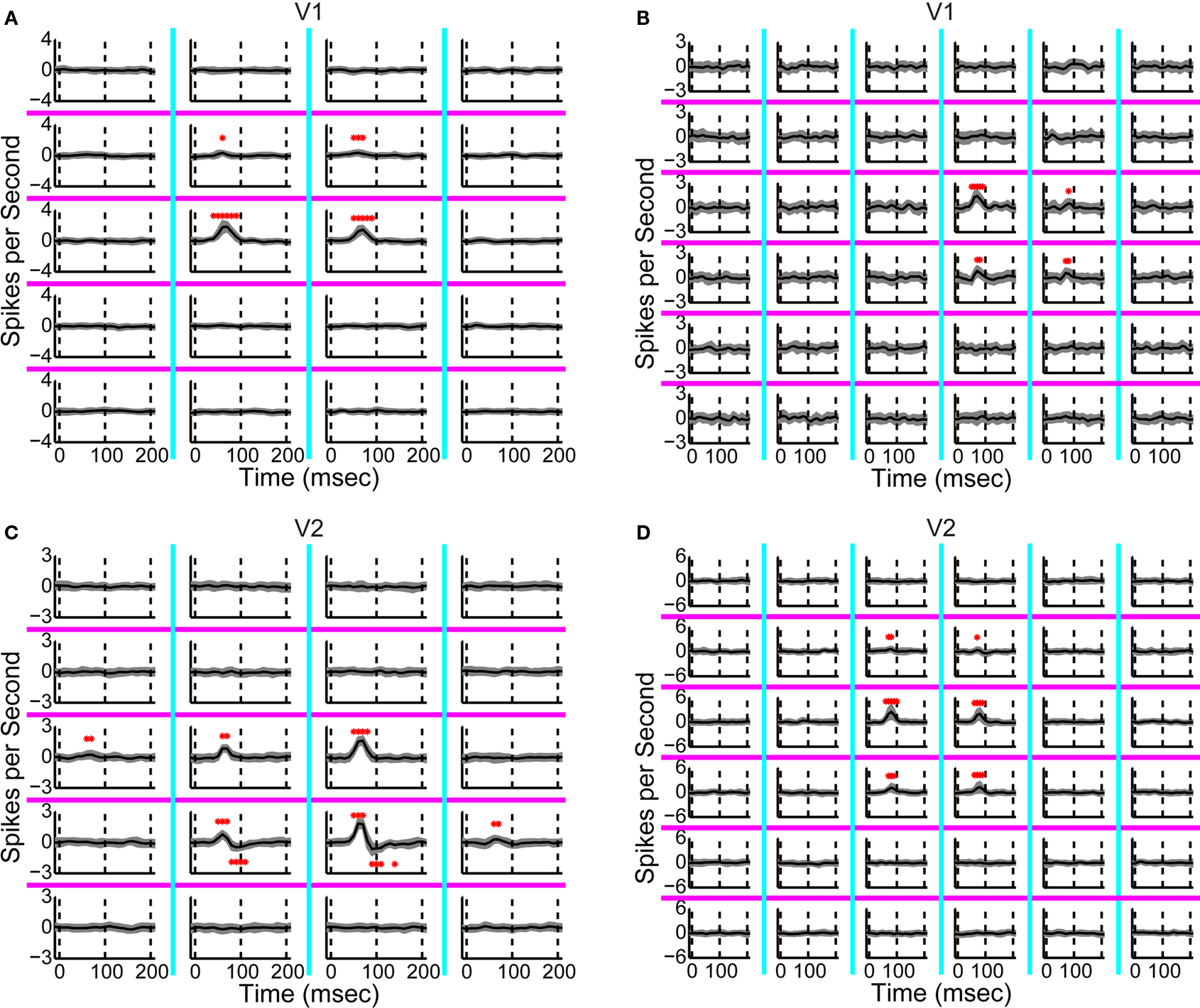
Figure 2. First-order response kernels. (A) First-order response kernels of a neuron in V1 measured using the 4 × 5 layout. The check size of the stimulus was 0.4 × 0.75 degrees of visual angle. The response kernel is plotted for each rectangular region in the stimulus; magenta and cyan lines correspond to subdivisions of the stimulus (compare Figure 1
A). The mean response kernel (of 32 repetitions) is plotted in black and the jackknife estimate of the standard deviation in gray. Asterisks mark timepoints at which the response was significantly different from zero (two-tailed t-test, α = 0.01, corrected for multiple comparisons). Dashed vertical lines show the timepoints 0, 100 and 200 ms. (B) First-order response kernels of another V1 neuron measured using the 6 × 6 layout. The check size of the stimulus was 0.4 × 0.4 degrees of visual angle. (C) First-order response kernels of a V2 neuron. The check size of the stimulus was 0.6 × 0.75 degrees of visual angle. (D) First-order response kernels of a V2 neuron. The check size of the stimulus was 0.4 × 0.2 degrees of visual angle.
The response timecourses in V1 and V2 showed three distinct patterns (Figures 3
A,B). Each trace was derived from one neuron – it is the normalized first-order kernel in the stimulus region that produced the largest RMS (root-mean-squared) response within the first 200 ms. As is shown, timing was very consistent across the population of 32 V1 neurons (Figure 3
A). In contrast, in the population of 28 V2 neurons (Figure 3
B), two distinct patterns of responses were seen: some were biphasic (colored in red), with an initial peak width narrower than the V1 responses; others were monophasic (colored in blue), with a peak width wider than the V1 responses. To support the observation that waveforms fell into three patterns, we performed a principal component analysis of the normalized kernels from both V1 and V2 (Figure 3
C). The insets labeled “PC 1” and “PC 2” show the first two principal components; the main figure shows the first and second component scores (the contributions of each of these components to the observed waveforms). Notably, PC 1 was biphasic and PC 2 was monophasic.
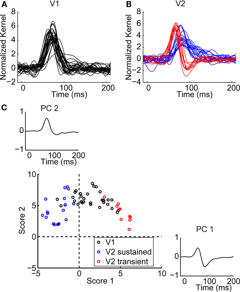
Figure 3. Population summary of first-order kernels. (A) Normalized first-order response kernels of V1 neurons. (B) Normalized first-order response kernels of V2 neurons, monophasic responses are colored blue and biphasic responses red. (C) First and second scores of PCA decomposition of all normalized first-order kernels. The principal components are plotted in insets along the corresponding axes. V1 kernels are colored in black; biphasic V2 kernels (first score larger than 0) in red; monophasic V2 kernels (first score smaller than 0) in blue.
The V1 population formed a single cluster, with large contributions of the second (monophasic) principal component and small contributions of the first (biphasic) principal component. The V2 population though, fell into two distinct clusters. One cluster had positive first scores (red markers); while the second cluster had negative first scores (blue markers). The difference between the two subpopulations in V2 was significant for the first score (Kolmogorov–Smirnov, p < 0.01). Because of the relative timing of the first and second components, the combination of a positive first score (biphasic, first positive then negative) and positive second score (monophasic positive), results in a transient biphasic response. Adding a negative first score (biphasic, first negative then positive) to a positive second score results in a sustained monophasic response. Therefore, we will call these clusters the “transient” and “sustained” V2 neurons, respectively. Out of 28 V2 neurons, 10 fell into the transient cluster and 18 into the sustained cluster. The bimodality of the first score for V2 was statistically significant (p < 0.01, Hartigan’s dip test, (Hartigan and Hartigan, 1985
). The distribution of first scores for V1 neurons on the other hand was unimodal (Hartigan’s dip test, p > 0.5). The above pattern of clustering was robust: it was also seen when we considered all significant responses (and not just the largest one from all regions in the stimulus, as in Figure 3
), and also, when the analysis was performed without normalization for response size.
The average V1 response was positive and became significant at a latency of 54 ± 11 ms (mean ± standard deviation). It had a positive peak at 70 ± 7 ms. The sustained V2 neurons had a slower and more sustained response; the latency of the first significant response was at 68 ± 9 ms and the peak was at 83 ± 6 ms. The transient V2 neurons started responding at 48 ± 15 ms, had a positive peak at 65 ± 5 ms and a negative peak at 95 ± 5 ms latency. The latencies of the first significant responses as well as the peak latencies were significantly later for the sustained V2 neurons than both V1 and V2 transient neurons (Kruskal–Wallis non-parametric ANOVA, p < 0.01).
To further delineate the difference between the three groups of neurons, we calculated their positive power (RMS of positive parts of the response kernel), and, similarly, their negative power. The positive power can be viewed as an overall measure of the expected preference for the preferred orientation over the orthogonal orientation; the negative power quantifies any “paradoxical” preference for the orthogonal orientation. We found that the positive power was not significantly different for the three groups, but the negative power was significantly larger for V2 transient responses (transient V2 neurons: median 0.078, lower quartile (l.q.) 0.017, upper quartile (u.q.) 0.39 spikes/s; sustained V2 neurons: median 0.014, l.q. 0.0004, u.q. 0.045 spikes/s; V1 neurons: median 0.007, l.q. 0.001, u.q. 0.077 spikes/s; Kruskal–Wallis nonparametric ANOVA, p < 0.01).
The overall responsiveness, measured as the mean firing rate in response to the stimulus, was not significantly different for the three groups (transient V2 neurons: median response of 5.6, l.q. 1.2, u.q. 21.3 spikes/s; sustained V2 neurons: median 3.4, l.q. 0.14, u.q. 15.2 spikes/s; V1 neurons: median 2.10, l.q. 0.08, u.q. 18.2 spikes/s).
Response Characteristics were Consistent Across Animals, and not Due to Stimulus Parameters
The different types of V2 responses were consistent across animals, but also had a tendency to cluster anatomically. In particular, the 10 transient neurons were found in 2 animals and 3 different recording sites, and the 18 sustained neurons were found in 3 animals and 7 different recording sites; the animal in common had both types of responses, but at different recording sites. In general, at each recording site we found one or the other of the two subpopulations of neurons, suggesting that neurons of each type seem to cluster together anatomically.
Since the stimuli were designed to fit the receptive field size, differences in the choice of stimulus parameters might contribute to the differences between responses of V2 subpopulations. However, there was no significant difference between the spatial parameters of the stimuli used for transient versus sustained V2 neurons, in terms of patch height and width (scaled to the receptive field) and spatial frequency (matched to the neuron’s tuning).
Because the receptive field sizes in V2 were larger than in V1, there was a significant difference between the stimuli used in V1 versus V2 (Kolmogorov–Smirnov, p < 0.05) for all three spatial parameters. But this was also not the source of the difference in response dynamics. To determine this, we analyzed the responses of 7 V1 neurons that responded to a stimulus designed for a simultaneously-recorded V2 neuron. We did not record from those 7 neurons with stimuli specifically designed for them, so we could not compare the responses of the same neurons to both types of stimuli. Instead we compared the normalized responses of these 7 V1 neurons to stimuli optimized for a V2 neuron with the normalized responses of all 32 V1 neurons recorded with their V1-optimized stimuli (Figure 3
A). The dynamics of the first-order kernels of these 7 V1 neurons in response to V2-optimized stimuli were the same as the responses of the 32 V1 neurons in response to V1-optimized stimuli. Specifically, the responses were positive monophasic, had a first significant positive response at 61 ± 7 ms, and a peak latency of 74 ± 5 ms. These were not significantly different than the V1 responses to V1-optimized stimuli (Kolmogorov–Smirnov, p > 0.3).
Spatial Interactions
To determine whether the above differences in response dynamics simply reflected an overall difference in response dynamics, or rather, was part of a more pervasive difference in the computations carried out by the neurons, we examined interactions within the receptive field – that is, how the response to a pair of regions (separated in space or time) differed from the sum of the responses to the two regions presented independently. To capture these interactions, we calculated second-order kernels. The second-order kernels compare the average response when the orientation in the two regions matched (either both preferred or both orthogonal), to the average response when the orientations differed (one preferred, one orthogonal). Because each side of the comparison contains the same contributions from preferred and orthogonal orientations considered independently, the second-order kernel isolates their interaction.
We consider spatial interactions in this subsection, and temporal interactions in the section “Spatial Interactions”. As diagrammed in Figure 1
C, each spatial second-order kernel compared the response to two neighboring regions filled with gratings of the same orientation versus the two regions filled with different orientations.
Spatial interactions in V1 and V2 differed in a manner that parallels what we found in the first-order kernels. Figure 4
A shows all nearest-neighbor second-order kernels for a neuron in V1. The peak of the response kernel for the interaction between two center regions was positive in sign (asterisks above the response kernel). This positivity means that there was a larger response when patches in the two halves of the receptive field had the same orientation, than when they differed. That is, this cell preferred continuous orientations over discontinuous ones, and this preference was more than the result of adding local orientation signals. Other second-order kernels were zero, indicating that other local orientation signals simply added up, without interacting. The same holds for the responses of another V1 neuron (Figure 4
B). In this case, we used the 6 × 6 setup so that a 2 × 2 grid was within the receptive field, and focus on the second-order kernels within a 4 × 4 subregion centered on the receptive field. There were significant interactions across two pairs of pixels. Both interactions had positive peaks, and both occurred across boundaries orthogonal to the receptive field (plotted on top of cyan lines). Thus, they too augmented the response to continuous orientations.
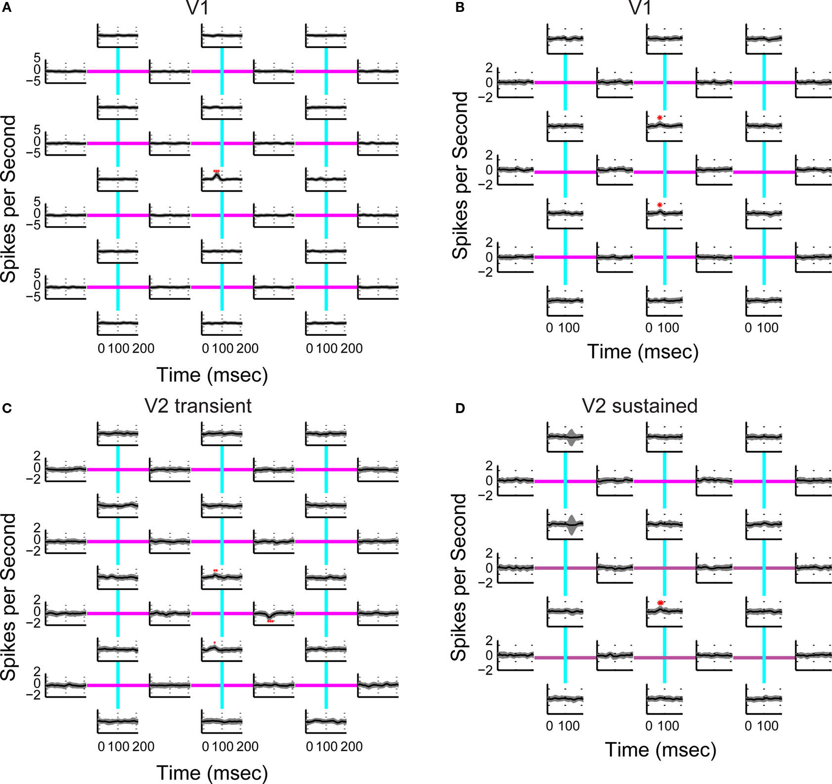
Figure 4. Spatial second-order response kernels. (A) Second-order response kernels of a neuron in V1. The check size of the stimulus was 0.4 × 75 degrees of visual angle. Colored lines depict the boundaries between the 20 regions, the cyan lines stand for boundaries orthogonal to the receptive fields preferred orientation and magenta lines for those parallel. The response kernels are plotted on the line corresponding to the boundary between the corresponding two neighboring regions. The mean response kernel (of 32 repetitions) is plotted in black and the jackknife estimate of the standard deviation in gray. Asterisks mark timepoints at which the response was significantly different from zero (two-tailed t-test, α = 0.01, corrected for multiple comparisons). Dashed vertical lines show the timepoints 0, 100 and 200 ms. (B) Second-order response kernels of another neuron in V1. The layout was 6 × 6 and the check size of the stimulus 0.4 × 0.4 degrees of visual angle. Only kernels for a 4 × 4 subregion centered on the receptive field are shown. (C) Second-order response kernels of a ‘transient’ neuron in V2 (same as in Figure 2
C). (D) Second-order response kernels of a “sustained” neuron in V2. The layout was 6 × 6 and the check size of the stimulus 0.4 × 0.2 degrees of visual angle. Only kernels for a 4 × 4 subregion centered on the receptive field are shown. The large standard deviation, without significant change in the mean response, in two of the subpanels in panel (D) stem from first-order responses that have been removed by the inverse-repeat method, not random variation (see “Stimulation with Orientation-Discontinuity Stimuli”).
In contrast, a typical transient V2 neuron (Figure 4
C) showed different preferences: while it had positive-going second-order responses indicating a preference for continuous orientations between some regions, it also had a kernel with a peak in the negative direction (asterisks below the response kernel). This was across a boundary parallel to the neuron’s preferred orientation (plotted on top of a magenta line), and indicates a preference for an orientation-discontinuity. This interaction occurred between two regions which both elicited a first-order response (Figure 2
C shows the first-order responses of the same neuron). The second-order responses of a sustained V2 neuron (Figure 4
D, plotted for a 4 × 4 subregion containing the receptive field) looked similar to the V1 neurons in that they were positive, and only occurred across boundaries orthogonal to the receptive field.
To summarize the population behavior, we chose the largest spatial second-order kernel for each neuron, separately considering interactions across boundaries orthogonal (Figures 5
A–C) and parallel (Figures 5
D–F) to the receptive field. Across boundaries orthogonal to the receptive field, the population response in V1 had a monophasic positive peak (Figure 5
A), which means that V1 cells preferred continuous orientations. On the other hand, transient V2 neurons showed a biphasic time course for their interactions (Figure 5
B): a positive peak followed by a negative one. Thus, in a patch of two regions separated by a boundary orthogonal to the receptive field, the second-order responses in those V2 neurons were best driven by an orientation-discontinuity followed by continuing orientation. Sustained V2 neurons had a weak spatial second-order response to this stimulus (Figure 5
C). The responses of V1 neurons, V2 transient and V2 sustained neurons were all significantly different from each other (Fisher Linear Discriminant analysis in the 2D space of first two principal components, explaining 75% of variance, p < 0.05, Bonferroni-corrected).
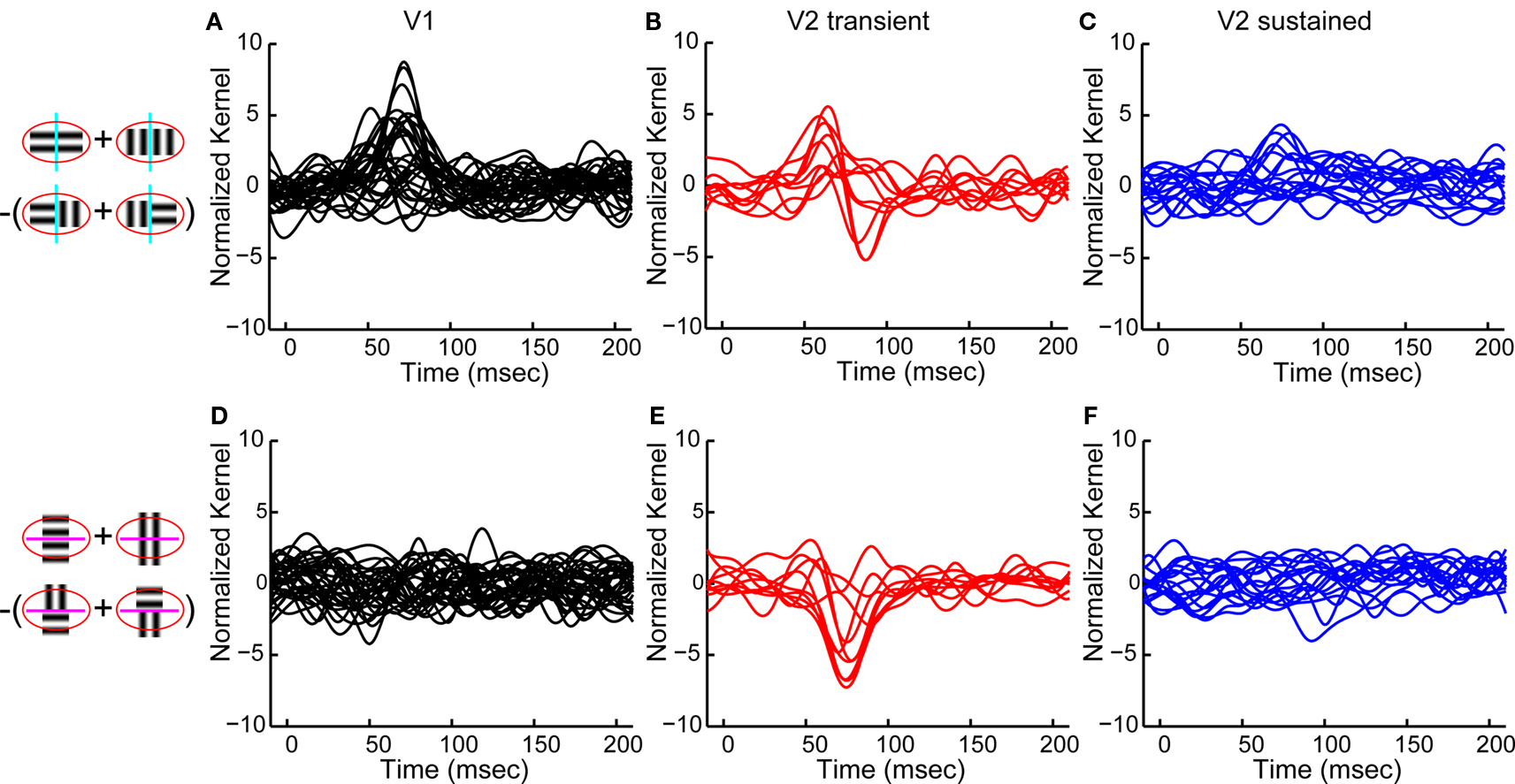
Figure 5. Population summary of spatial second-order response kernels. Schematics on the left illustrate the computations of spatial second-order responses across boundaries orthogonal to the receptive field (top, cyan lines), and across boundaries parallel to the receptive field (bottom, magenta lines). The red ellipse stands for the classical receptive field. (A) Normalized second-order response kernels across boundaries orthogonal to the receptive field for all V1 neurons (largest response for each neuron). (B) Same as (A) for transient V2 neurons. (C) Same as (A) for sustained V2 neurons. (D) Normalized second-order response kernels across boundaries parallel to the receptive field for all V1 neurons (largest response for each neuron), (E) Same as (D) for transient V2 neurons. (F) Same as (D) for sustained V2 neurons.
Not all neurons had measurable second-order spatial interactions across boundaries orthogonal to the receptive field. For V1 neurons, 14 out of 32 neurons showed a significant response; for transient V2 neurons, 5 out of 10; for sustained V2 neurons, only 3 out of 18. The latency of the peak for all significant responses was 62 ± 17 ms in V1, 60 ± 0 ms in transient V2 neurons and 83 ± 2 ms for sustained V2 neurons.
The character of the spatial second-order responses allows us to draw inferences about likely mechanisms. In V1, their characteristics were simple: they were always of positive sign and their waveform was similar to that of the first-order response. This suggests a simple explanation: they could arise from a threshold nonlinearity. Specifically, simultaneous presence of the preferred orientation in two adjacent regions overcomes the threshold, which manifests as a supralinear response. Consistent with this mechanism, the peak latency of this second-order response (62 ± 17 ms) was similar to the latency for the first-order response (70 ± 7 ms).
However, the interaction between subregions within the receptive field appeared only when the subregions were placed across boundaries that were orthogonal and not parallel to the receptive field. If the interaction is simply the result of a threshold, then it should also occur between two regions that are adjacent along a parallel border. As seen in Figure 5
D, it did not. This observation suggests that the spatial second-order responses seen in our V1 experiments might be generated by iso-orientation facilitation (Nelson and Frost, 1985
; Kapadia et al., 1995
, 2000
; Polat et al., 1998
).
For interactions across boundaries parallel to the receptive field, there was a marked difference between V1 and transient V2 neurons. Most (7/10) transient V2 neurons response kernels had a strong negative peak (Figure 5
E). This means that transient V2 neurons had a nonlinearity sensitive to orientation-discontinuities parallel to their receptive field orientation, augmenting their responses to discontinuities. All of these interactions were between regions that elicited a positive first-order response. In contrast, only 3 out of 32 V1 neurons had a significant second-order response across these boundaries and none of 18 sustained V2 neurons did (Figure 5
F).
The latency of the negative peak for the transient V2 neurons with significant responses was 77 ± 8 ms. This latency was significantly later than the positive peak for the first-order response in the same neurons, which was 64 ± 5 ms (paired t-test, p < 0.01, N = 7, average time difference 13 ± 8 ms). Because of this temporal separation, it is unlikely that this second-order response was produced merely by a threshold or saturation nonlinearity.
For regions that were not directly adjacent (e.g. diagonally-related regions and next-nearest-neighbor regions), we found no measurable interactions in V1 and V2.
Temporal Interactions
Next, we consider temporal interactions (Figure 1
D). Above (Figure 3
), we have shown that transient V2 neurons typically had biphasic first-order kernels, indicating that they preferred a change of orientation to the static presentation of an oriented grating. The temporal second-order kernels show that this preference is augmented by nonlinear interactions across time, and also differentiate the transient and sustained subpopulations.
For a typical V1 neuron, the two central regions elicited a biphasic temporal second-order response, consisting of a positive peak followed by a negative one (Figure 6
A). This means (see caption of Figure 1
for sign convention) that the initial response was enhanced if the same orientation was presented (the short-latency positive component), but the later portion of the response was enhanced when the orientation was changing (the longer-latency negative component). A typical V2 neuron only had the negative peak, meaning that it preferred changing orientations throughout its response time course (Figure 6
B). Note that the preferences isolated by this kernel go beyond those implied by the first-order kernel: these responses represent interactions, and cannot be generated by mechanisms that merely sum a changing orientation preference over time. This pattern was seen in the 7 of 32 V1 neurons that had a significant second-order temporal interaction (Figure 6
C).
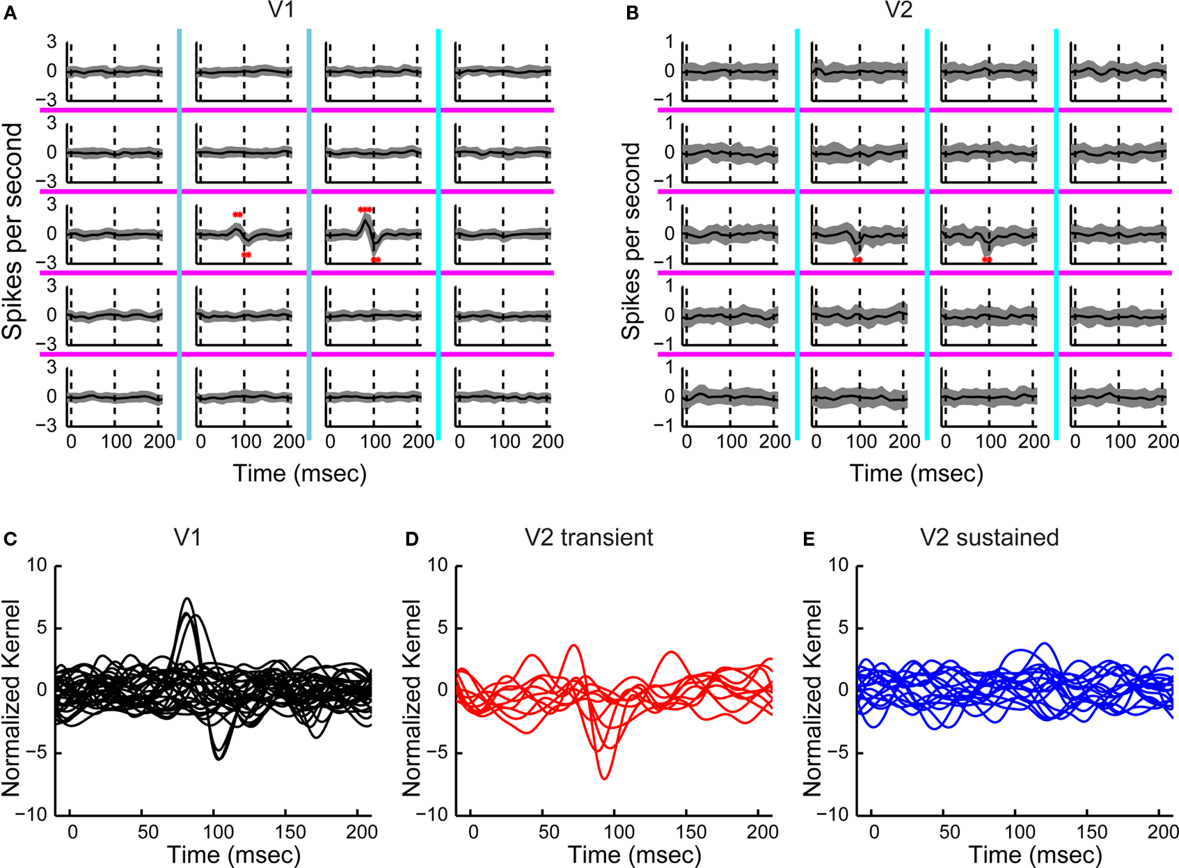
Figure 6. Temporal second-order responses. (A) Temporal second-order responses of a V1 neuron. The check size of the stimulus was 0.4 × 0.75 degrees of visual angle. Each trace shows the interaction of stimulus frames at two successive times: the difference between the response when the orientation was the same in successive frames, and the response when the stimuli change orientation in successive frames. The mean response kernel (of 32 repetitions) is plotted in black and the jackknife estimate of the standard deviation in gray. Asterisks mark timepoints at which the response was significantly different from zero (two-tailed t-test, α = 0.01, corrected for multiple comparisons). Dashed vertical lines show the timepoints 0, 100 and 200 ms. (B) Temporal second-order responses of a V2 neuron. The check size of the stimulus was 0.4 × 1.1 degrees per visual angle. (C) Normalized temporal second-order response kernels (largest response) for all V1 neurons. (D) Same as in (C) for V2 transient neurons. (E) Same as in (C) for V2 sustained neurons.
In V2 temporal interactions had different dynamics, and also distinguished the two subpopulations. Six of the 10 transient V2 neurons had a significant response (Figures 6
B,D) consisting of a negative peak, while only 2 of 18 sustained neurons had a significant response (Figure 6
E). The responses of V2 transient neurons were significantly different from the responses of V2 sustained neurons as well as from responses of V1 neurons (Fisher Linear Discriminant analysis in the 3D space of first three principal components (explaining 67% of variance), p < 0.05, Bonferroni-corrected). The incidence of significant temporal interactions was also greater in V2 transient neurons than V2 sustained neurons or V1 neurons (contingency table analysis, p < 0.01).
The latency of the positive peak for the 7 V1 neurons was 79 ± 30 ms, for the transient V2 neurons the positive peak was at 95 ± 68 ms and the negative peak was at 130 ± 55 ms.
Surround Suppression and Standard Tuning Properties were Similar in the Two V2 Subpopulations
The fact that transient V2 neurons showed spatial interactions, that sustained V2 neurons did not, raises the question whether there is a connection with known contextual modulations. Surround suppression is of particular interest, because some forms of surround suppression (Allman et al., 1985
; Polat, 1999
; Fitzpatrick, 2000
; Series et al., 2003
; Bair, 2005
; Angelucci and Bressloff, 2006
) are nonlinear phenomena that could contribute to interactions between patches of different orientations. However, there was no difference in strength of suppression measured with standard techniques (see Materials and Methods) between the two different neuronal subpopulations (Kolmogorov–Smirnov test, p > 0.5). Transient V2 neurons had a median suppression index of 0.0, with a lower quartile (l.q.) of 0.0 and an upper quartile (u.q.) of 0.20. Sustained V2 neurons had a median of 0.16 (l.q. 0, u.q. 0.50). The same holds for measurements of end-stopping and side suppression separately. Thus, the different types of response dynamics do not appear to be related to any of several previously-described forms of surround suppression – the subpopulations were quite similar in this regard.
We also did not find any significant differences between the subpopulations in V2 for receptive field size, preferred spatial frequency and temporal frequency, direction selectivity, F1/F0 ratio, or orientation tuning width.
Laminar Location and Response Latency
We were able to reconstruct the laminar position for all 32 neurons in V1 and 28 neurons in V2. In V1, we found 12 neurons in layer 4, 9 neurons in layer 2/3 and 6 neurons in layer 6. Five neurons were in the vicinity of the boundary between layers 2/3 and 4.
In V1, there was a difference in timing of the response in that the neurons in layer 4 have significantly earlier peak latencies than neurons in layers 2/3 or 6 (layer 4: 66 ± 5 ms, layer 2/3: 73 ± 7 ms, layer 6: 73 ± 5 ms, ANOVA, p < 0.05). Also the latency of the first significant positive response (two-tailed t-test, α = 0.01, corrected for multiple comparisons) was significantly earlier in layer 4 than in layer 6 (layer 4: 45 ± 12 ms, layer 2/3: 53 ± 16 ms, layer 6: 62 ± 4 ms, ANOVA, p < 0.05).
In V2, 7 transient neurons were found in layer 2/3, and 3 in layer 4. Nine sustained V2 neurons were found in layer 2/3, 3 in layer 4, 3 in layer 5 and 3 neurons were in the vicinity of the boundary between layers 2/3 and 4. There was no layer specificity for the transient versus sustained neurons (contingency table analysis, p = 0.34). However, the peak latency was significantly different between layers as well as groups (2-way ANOVA, p < 0.05). Overall, layer 2/3 showed significantly shorter peak latencies than layer 4 and the responses of transient neurons were significantly faster than of sustained neurons (Multiple comparisons according to Tukey–Kramer, p < 0.05). The peak latency was shortest in layer 2/3 transient neurons (63 ± 5 ms), followed by layer 4 transient neurons (70 ± 0 ms). The next groups were the layer 2/3 sustained neurons with (80 ± 0 ms), the layers 5 sustained neurons (83 ± 6 ms), and the layer 4 sustained neurons (90 ± 1 ms). The latency of the first significant response was not significantly different between layers, but between neuron types: transient neurons had an onset time of 46 ± 14 ms, and sustained neurons 69 ± 10 ms.
In summary, the different types of V2 neurons did not correlate with laminar positions, and both types were present across several layers. There was a clear and measurable timing difference between the layers in V1 as well as in V2. In V1, the signal was fastest in layer 4, as expected, as the LGN input arrives in layer 4 (Lund, 1988
). In V2, the peak of the response was earlier in layer 2/3 than in layer 4, but the first significant response was not. This is at least partly consistent with anatomical studies that show that V1 input to V2 terminates in layers 3 and 4 (Rockland and Pandya, 1979
; Lund et al., 1981
; Weller and Kaas, 1983
; Van Essen et al., 1986
; Rockland and Virga, 1990
; Sincich and Horton, 2002
).
Signal Transformations
We now consider what kinds of transformations can produce the two kinds of V2 responses from the ones in V1. For the sustained V2 neurons, their first-order responses were qualitatively similar to those of V1 neurons, only slower. This suggests a simple and parsimonious explanation: sustained V2 neurons integrate V1 responses over space and time. Integration can also account for why the second-order responses for sustained neurons in V2 were nearly always insignificant – essentially, integration dilutes their contribution. To see this, consider first the spatial interactions. A specific spatial boundary orthogonal to the V2 receptive field would only elicit a nonlinear response from the V1 inputs that are lined up across this boundary. Since the V2 receptive field is larger than the V1 receptive field, only a small portion of the V1 inputs would be positioned to contribute to the second-order kernel, while all of the V1 inputs could contribute to the first-order kernel. Integration of V1 outputs in V2 also accounts for attenuation of second-order temporal kernels in V2. The temporal second-order kernels of V1 neurons are weak and biphasic; their integration over time by a V2 neuron will reduce their impact because positive phases from one neuron’s contribution will cancel the negative phases of another.
The responses of transient V2 neurons, on the other hand, require a different transformation of signals from V1. Qualitatively, the first-order responses of a typical transient V2 neuron look like the sum of a V1 responses and its derivative. This suggests that the V2 responses could be generated by combining an excitatory input from V1 with a delayed inhibitory input from the same source. As shown in Figure 7
B, this simple idea provides an accurate account of the first-order responses of V2 neurons, with a 10 ms delay and relative weights of the excitatory and inhibitory inputs in proportion ∼3:2 (Figure 7
A). Note that this is a functional account, and not one that implies a particular wiring diagram: we do not suggest that only one neuron excites and inhibits or that the connections are direct, and we do not know the anatomical location of the inhibitory neuron (and therefore diagram it as lying in between V1 and V2).
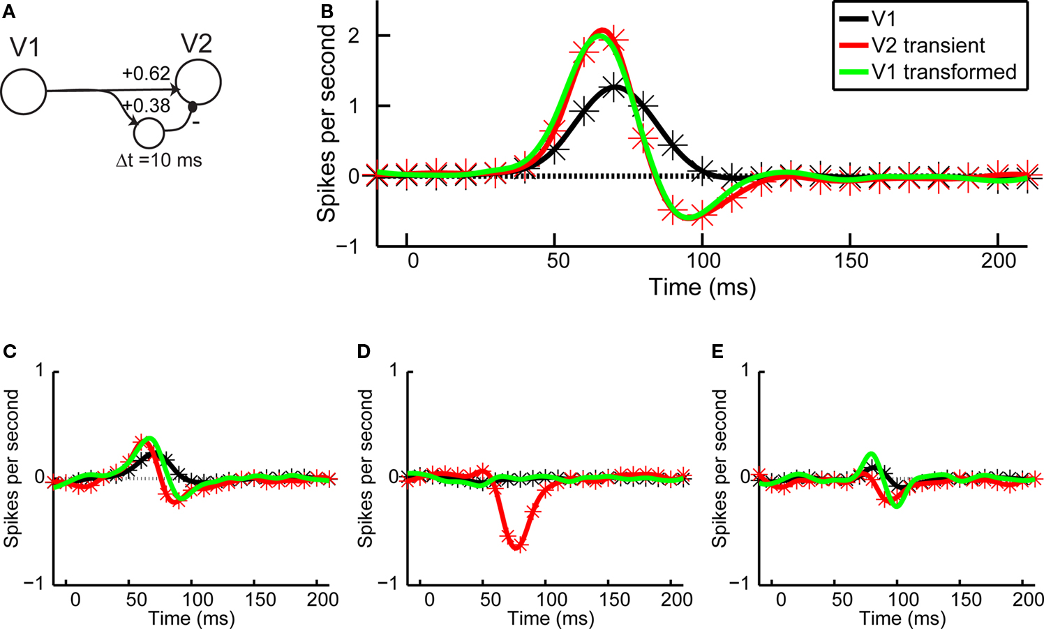
Figure 7. Average responses and V1–V2 transformation. (A) Schematic of the conceptual transformation of V1 responses into V2 responses, with parameter values as computed by fitting the first order responses shown in panel (B). (B) Average first-order responses for V1 (black) and transient V2 (red). The solid green line is the V1 response transformed according to the scheme of panel (A). (C) Average second-order responses across boundaries orthogonal to the preferred orientation for V1 (black) and transient V2 (red), and the transformed V1 signal (green). (D) Same as in (C), but for second-order responses across boundaries parallel to the preferred direction. (E) Same as in (C), but for temporal second-order responses.
Given this close fit, it is logical to ask whether the same transformation can also account for the second-order responses in V2. If so, we could account for both the linear and nonlinear components of V2 simply by temporal filtering of signals arising in V1. Conversely, to the extent that this transformation does not account for second-order responses, we can infer the properties of new nonlinear components generated in the transformation from V1 to V2. As shown in Figures 7
C–E, we find that the transformation cannot account for the shape of the spatial second-order responses in V2. It fails modestly for the spatial second-order responses across boundaries orthogonal to the receptive field (Figure 7
C) as well as for the temporal second-order responses (Figure 7
E) and more dramatically for the spatial second-order kernels parallel to the receptive field (Figure 7
D). The latter failure can be anticipated from the qualitative nature of our results: since V1 neurons had no second-order interactions parallel to the receptive field, a linear transformation can not possibly produce an interaction in V2.
Summary of Findings
Our main result is that V2 neurons can be divided into two subpopulations (“sustained” and “transient”), based on qualitative differences in the dynamics of their responses to small patches of gratings. These dynamical differences encompass responses to individual grating patches (“first-order”) and spatiotemporal interactions between two grating patches (“second-order”). These differences combine to allow the two subpopulations of cells to process spatial information in complementary fashions, thus enabling V2 to solve the problem of extracting texture boundaries de novo (the subpopulation that performs differentiation), while also preserving and even enhancing boundary information extracted in V1 (the subpopulation that performs integration).
The dynamics of the first-order responses indicates whether a neuron responds better to a grating patch whose orientation is constant over time, or whose orientation is changing. While all V1 neurons in our sample had temporally monophasic first-order responses, one subpopulation of V2 neurons (“transient”) had biphasic responses – first positive then negative – and the second subpopulation (“sustained”) had monophasic responses that were broader than the responses of V1 neurons. Thus, while V1 neurons and sustained V2 neurons simply responded better to their preferred orientation, transient V2 neurons responded best to the preferred orientation if it followed the non-preferred orientation. In other words, these V2 neurons responded best to a “switching on” of the preferred orientation, signaling a change in the visual input.
The spatial and temporal second-order response components accentuate the different ways in which these different kinds of neurons responded. V1 neurons had monophasic spatial second-order responses across boundaries orthogonal and none across boundaries parallel to the preferred orientation of the receptive field. These spatial second-order responses signify that the neurons responded better if the orientation was unchanging across space than if the orientation differed in adjacent patches.
Transient V2 neurons manifested two kinds of spatial interactions, and both reinforce their preference for orientation-discontinuities. Like the V1 neurons, they manifested spatial interactions across boundaries orthogonal to the receptive field. But unlike the V1 neurons, the time course of these responses was biphasic.
The second spatial interaction in transient V2 neurons is one that was not present in V1 neurons: monophasic, negative interactions across boundaries parallel to the receptive field. These also signify a preference for orientation-discontinuities that goes beyond merely summing excitatory and inhibitory influences. A nonlinearity of this kind, that augments the response to a texture boundary parallel to the receptive field, is also a characteristic reported by others using different kinds of stimuli (von der Heydt et al., 1984
, 2000
; Peterhans and von der Heydt, 1989
; Leventhal et al., 1998
; Marcar et al., 2000
; Song and Baker, 2007
). That the latency of the peak for this second-order response was significantly later than for the first-order response, shows that it cannot be explained by a simple threshold or saturation nonlinearity, but probably involves network interactions. This type of interaction was observed only between regions that elicited positive first-order responses, i.e. within the classical receptive field. This is in line with the observation that the transient V2 neurons did not show any increased amount of surround suppression, a well-known interaction between classical and non-classical receptive field (Allman et al., 1985
; Polat, 1999
; Fitzpatrick, 2000
; Series et al., 2003
; Bair, 2005
; Angelucci and Bressloff, 2006
).
Temporal second-order responses were biphasic for the V1 neurons. The positive component dominated, indicating that V1 neurons combined like-orientation signals supralinearly over time. In transient V2 neurons, the negative component dominated, indicating a nonlinearity that reinforces changes in orientation.
In the spatial and temporal domain, sustained V2 neurons manifested only very weak second-order interactions, indicating that they integrate signals from the grating patches linearly over time as well as over space.
The two subpopulations of neurons in V2 did not differ in their general tuning properties. However, there was a significant difference in response latency between the two groups, with shorter latencies in the transient neurons. Anatomical studies show that thick stripes in V2 get their main input from layer 4 in V1, whereas thin and pale stripes receive input mainly from layer 2/3 in V1 (for reviews see Livingstone and Hubel, 1988
; Sincich and Horton, 2005
). Therefore, we hypothesize that transient neurons are in thick stripes and get faster input from layer 4.
Comparison with Other Studies; Receptive Field Subregions and Surround Suppression
Two recent studies (Nishimoto et al., 2006
; Anzai et al., 2007
) also analyzed the computations performed by extrastriate neurons to boundary extraction. Both studies identify spatial inhomogeneities of orientation tuning in the receptive fields of a fraction of striate and extrastriate neurons – in one study via local spectral reverse correlation (Nishimoto et al., 2006
), and in the other via the use of grating patches (Anzai et al., 2007
). Because the latter used grating patches, they were able to focus on the detailed tuning properties of receptive field subregions, and found that about 30% of neurons in V2 were tuned to different orientations, commonly about 90° apart. Because of stimulus differences, the studies are not directly comparable. Nevertheless, one may speculate that the transient subpopulation (10/28 V2 neurons) identified here have subregions that respond to non-preferred orientations under the stimulus conditions of the other studies, because they have evidence of a latent sensitivity to orthogonal orientations when their dynamics are probed.
Whereas Anzai et al. propose several different possible mechanisms for tuning to combinations of orientations (Anzai et al., 2007
), these mechanisms are all based on the assumption that the feedforward input from V1 to V2 is purely excitatory. In contrast, the present focus on dynamics suggests a simple, stereotyped transformation of information from V1 to V2. For the sustained V2 neurons, spatiotemporal integration accounts for all of the main features of the response. For the transient V2 neurons, combination of antagonistic influences provides a complete account for the linear portion of the response, and a partial account of the second-order portion. This spatiotemporal differentiation of V1 inputs as a building block of the V2 response is a concept that has not been proposed prior to this study.
Surround suppression likely contributes to boundary analysis, and is present already in V1 (Allman et al., 1985
; Polat, 1999
; Fitzpatrick, 2000
; Series et al., 2003
; Bair, 2005
; Angelucci and Bressloff, 2006
). While many of our V1 neurons (70%) manifested surround suppression when probed with full-field gratings (median surround suppression 0.23, l.q. 0, u.q. 0.43), it might appear surprising that it was not manifest in the responses to the orientation-discontinuity stimuli. For example, surround suppression that is selective for the preferred orientation (DeAngelis et al., 1994
; Cavanaugh et al., 2002
) would be expected to cause negative first-order and/or negative spatial second-order kernels. We did not observe such responses with the orientation-discontinuity stimuli.
Since we did find surround suppression when studying these neurons with standard gratings, the absence of manifestations of surround suppression must be due to the characteristics of the orientation-discontinuity stimuli, rather than some idiosyncrasy of cell selection or physiology. Indeed, the orientation-discontinuity stimuli differed from stimuli that elicit surround suppression both temporally and spatially. Iso-orientation surround suppression achieves its maximum strength on average within 50 ms from stimulus onset (Bair et al., 2003
); our frame time was 20 ms. In experiments using the present stimuli but with longer frame times (40 ms), we found more significant second-order responses of negative sign (data not shown), supporting the relevance of temporal factors. In addition to the temporal differences, there are spatial differences between the orientation-discontinuity stimuli and standard gratings. Each patch covers only a fraction of the whole surround, and it is possible that surround must be stimulated coherently in order to elicit surround suppression.
We did not find V1 neurons that responded to orientation-discontinuities with increased firing rates, a contextual modulation that is most likely generated by either lateral interactions in V1 or feedback from V2 to V1 (Lamme, 1995
; Zipser et al., 1996
). One possible reason for this discrepancy is that we used anesthetized animals and therefore attentional effects played no role. However, even with controlled attention away from the stimulus (Marcus and Van Essen, 2002
) as well as with anesthetized animals, this contextual effect is observed (Sillito et al., 1995
; Schmid, 2008
).
That we did not observe increased firing rates with orientation-discontinuities in V1 could be due to the short frame times used in this study (20 ms). Response enhancement in V1 neurons has a latency of 30–40 ms relative to the onset of the neuronal response itself (Lamme, 1995
). As with surround suppression, it is possible that the short frame-rate is not enough to drive relatively slow processes such as lateral interactions. Since these contextual effects are directly related to surround suppression (Schmid, 2008
), it is possible that the short frame times used here is responsible for both types of discrepancies with other studies. Feedback from V2 to V1 is more rapid (Girard et al., 2001
) and should therefore be recruited with our stimuli. However, we did not see any contextual effects in V1, such as increased firing rates for orientation-discontinuities, that would be consistent with such rapid feedback from V2 to V1. This is in agreement with the observation that deactivation of area V2 does not affect response modulations due to texture discontinuities in V1 (Hupe et al., 2001
).
Temporal and Spatial Change Detection Mechanism
We suggest that the phenomenological temporal differentiation seen in V2 is accomplished in the brain by feedforward excitation followed by delayed inhibition. Feedforward excitation followed by inhibition from the same source could arise from a microcircuit consisting of monosynaptic excitation and disynaptic inhibition, as found throughout the brain (Toyama et al., 1974
; Frotscher, 1989
; Kita et al., 2005
; Verbny et al., 2006
; Silberberg and Markram, 2007
). Such a microcircuitry has recently been proposed as a mechanism for detecting abrupt changes in the sensory world (Bouaouli and Deneve, 2009
).
Spatial differentiation, however, cannot be explained by such a simple transformation, because it is associated with the emergence of (nonlinear) spatial interactions. At a computational level, the transformation thus resembles those that have been invoked to account for processing of second-order stimuli (Chubb and Sperling, 1988
; Voorhees and Poggio, 1988
; Cavanagh and Mather, 1989
; Graham et al., 1992
; Wilson et al., 1992
; Wolfson and Landy, 1995
; Baker, 1999
; Baker and Mareschal, 2001
). The unifying concept of these models is a set of filters followed by a nonlinearity followed by a second set of filters, which basically performs a differentiation operation. While all these models are based on psychophysics as well as theoretical considerations, our study is, to our knowledge, the first physiological study that directly demonstrates this differentiation operation.
While the spatial and temporal change detection can be modeled most easily using only feedforward mechanisms, we do not exclude the possibility that feedback from higher cortical areas than V2 might also be involved.
Methodological Innovation
The main methodological novelty presented in this study is the simultaneous evaluation of first-order and second-order responses in time and two spatial dimensions – crucial ingredients in building a model for the computations performed by V2 neurons. The barrier to doing this is that a large number of parameters need to be measured and evaluated with neural data with low signal-to-noise ratios; long measurements are required to reduce the noise. Other studies have approached this problem (studying complex cells in primary visual area V1) by using one-dimensional random bar stimuli (Emerson et al., 1987
; Touryan et al., 2002
; Rust et al., 2005
) or 2D random dot stimuli (Gaska et al., 1994
; Livingstone and Conway, 2003
; Sasaki and Ohzawa, 2007
). Our approach is different in several ways. Firstly, we used m-sequences, which have the advantage that unlike with Gaussian white noise stimuli, random correlations are not presented. The use of m-sequences, whose autocorrelation is very close to a delta function, results in high signal-to-noise ratios even with few repetitions and this allow us to measure the first-order along with several second-order responses simultaneously. We deal with the problem of separately measuring all of the relevant first- and second-order responses (i.e. the “overlap problem” see “Stimulation with Orientation-Discontinuity Stimuli”) by tailoring the m-sequence to the specific demands of the experiment. Secondly, the stimuli are two-dimensional like the random dot stimuli, but the individual elements in our stimuli are not dots but patches of oriented gratings. This design allows us to focus on the processing of orientation signals in V1 and V2 neurons.
Conclusion
Our results identify two subpopulations of orientation-selective neurons in area V2 that process orientation signals in a complementary fashion. The sustained V2 neurons integrate orientation signals over space and time. Their responses can be understood as integration of outputs of V1 receptive fields with similar orientation tuning over an extended period in time. These neurons would be expected to signal long luminance boundaries or surfaces of objects with extended regions of uniform texture that are constant in time. Responses of the transient neurons can be understood as a spatial and temporal spatial derivative of the V1 responses in combination with simple nonlinearities. These neurons may play a major role in the early visual system’s detection of orientation change in time and boundaries defined by differences in orientation. More broadly, by delineating the spatial and temporal interactions between receptive field subregions, our findings identify two distinct types of transformations carried out between the visual areas V1 and V2, and enable V2 to extract texture boundaries (differentiation) while simultaneously building on the boundary information extracted in V1 (integration).
The authors declare that the research was conducted in the absence of any commercial of financial relationships that could be construed as a potential conflict of interest.
This work is supported by NIH grant R01EY09314 to JV.