 Levin Kuhlmann
 Trichur R. Vidyasagar*
- Department of Optometry and Vision Sciences, The University of Melbourne, Parkville, VIC, Australia
Controversy remains about how orientation selectivity emerges in simple cells of the mammalian primary visual cortex. In this paper, we present a computational model of how the orientation-biased responses of cells in lateral geniculate nucleus (LGN) can contribute to the orientation selectivity in simple cells in cats. We propose that simple cells are excited by lateral geniculate fields with an orientation-bias and disynaptically inhibited by unoriented lateral geniculate fields (or biased fields pooled across orientations), both at approximately the same retinotopic co-ordinates. This interaction, combined with recurrent cortical excitation and inhibition, helps to create the sharp orientation tuning seen in simple cell responses. Along with describing orientation selectivity, the model also accounts for the spatial frequency and length–response functions in simple cells, in normal conditions as well as under the influence of the GABAA antagonist, bicuculline. In addition, the model captures the response properties of LGN and simple cells to simultaneous visual stimulation and electrical stimulation of the LGN. We show that the sharp selectivity for stimulus orientation seen in primary visual cortical cells can be achieved without the excitatory convergence of the LGN input cells with receptive fields along a line in visual space, which has been a core assumption in classical models of visual cortex. We have also simulated how the full range of orientations seen in the cortex can emerge from the activity among broadly tuned channels tuned to a limited number of optimum orientations, just as in the classical case of coding for color in trichromatic primates.
1 Introduction
Understanding the neural representation of a visual scene is a central problem in neuroscience. Probably, the most studied aspect of the neural representation of vision is visual orientation selectivity – OS (for reviews, see Vidyasagar et al., 1996; Sompolinsky and Shapley, 1997; Ferster and Miller, 2000). Having such neurons tuned to oriented visual information is important for providing a sparse, informative representation of the visual scene through the detection of edges of objects (Grossberg and Mingolla, 1985).
Orientation selective cells were first discovered in primary visual cortex (V1) of cats and monkeys through the pioneering studies of Hubel and Wiesel(1962, 1968). Hubel and Wiesel proposed that the response properties of simple cells emerged from the excitatory convergence of lateral geniculate nucleus (LGN) cells which have spatially offset, but aligned receptive fields (RFs). Studies that are taken as evidence for such a convergence model include demonstrations that recording of just the excitatory postsynaptic potentials to a cell by intracellular recordings (Ferster, 1986), inactivation of intra-cortical interactions (Ferster et al., 1996; Chung and Ferster, 1998; Kara et al., 2002) or the molecular blocking of cortical inhibition (Nelson et al., 1994), all still preserve the OS of simple cells. Reid and Alonso (1995) observed that LGN and simple cells showing correlated responses also show an overlap between the LGN ON or OFF centers and the corresponding ON or OFF subfields of the simple cell RF, respectively. Combined, these studies demonstrate that the feed-forward excitatory LGN inputs to a simple cell can exhibit orientation tuning (OT), but they do not establish how such selectivity is generated in the excitatory input.
Three common alternatives to the Hubel and Wiesel excitatory convergence model are that OS emerges from (1) intra-cortical inhibition (Creutzfeldt et al., 1974; Sillito, 1975; Sillito et al., 1980; Heggelund, 1981; Crook et al., 1998; Hirsch, 2003; Hirsch et al., 2003; Teich and Qian, 2006), (2) spatially offset ON and OFF LGN inputs (Schiller, 1982; Sherk and Horton, 1984; Miller, 1994; Hirsch, 2003; Martinez et al., 2005; Priebe and Ferster, 2005; Ringach, 2007; Westheimer, 2007; Jin et al., 2011), and (3) sharpening of the orientation-bias of LGN inputs (Vidyasagar and Urbas, 1982; Vidyasagar, 1984a, 1987; Vidyasagar and Heide, 1984; Vidyasagar and Siguenza, 1985; Soodak et al., 1987, 1991; Shou and Leventhal, 1989). This paper centers primarily on the third alternative, but also incorporates elements of the other two models as well. Though most retinal and LGN cells respond well to stimuli of any arbitrary orientation, the majority give stronger responses to stimuli of a preferred orientation, especially at higher spatial frequencies (Levick and Thibos, 1980; Vidyasagar and Heide, 1984; Passaglia et al., 2002; Xu et al., 2002). It has been proposed that interactions involving orientation-biased LGN cells could create the strong OS and spatial frequency (SF) tuning seen in cortex and that the same mechanisms can also explain the range of length–response functions observed for different simple cells (Vidyasagar, 1987; Vidyasagar et al., 1996). This paper codifies these ideas in a computational model that is consistent with current evidence.
2 Materials and Methods
We present a computational model where simple cells are excited by lateral geniculate cells with an orientation-bias and disynaptically inhibited by lateral geniculate cells with unoriented RFs (or biased fields pooled over orientation), both at approximately the same retinotopic co-ordinates. This interaction, combined with recurrent cortical excitation and inhibition and a power-law spike-rate response function is able to qualitatively account for the full gamut of OT, SF tuning, and length–response functions observed for simple cells and simple-like hypercomplex cells. Moreover, blocking inhibitory input to the simulated model simple, or simple-like hypercomplex, cell can account for the observed effects of iontophoretic application of bicuculline, a gamma-aminobutyric acid (GABA) antagonist, on OT, SF tuning, and length–response functions. The model can also describe the effects of electrical stimulation in the LGN during simultaneous visual stimulation on the orientation selectivity of LGN and simple cells. Models based on recurrent cross-orientation excitation and inhibition within the cortex have come to be called the recurrent model (RM; Teich and Qian, 2006). Therefore we refer to our model as the anisotropic LGN driven RM (or ALD-RM).
The computational model essentially consists of input, ON-center LGN cells, oriented excitatory simple cells, oriented inhibitory simple cells, and unoriented inhibitory cortical cells. Although for the sake of parsimony we focus only on the ON projection to cortex, our model is consistent with evidence about the projection of ON and OFF LGN cells onto cortex (see Discussion). In the following descriptions we may use the phrases “LGN cell” and “LGN field” interchangeably, while generally meaning an LGN field, since a particular RF may be common to as many as 6–20 LGN cells due to the divergence in the retinogeniculate projection (Friedlander et al., 1981). Since there is good evidence for a robust convergence of about 10 LGN cells on to a layer IV stellate cell in the cat striate cortex (Tanaka, 1983; da Costa and Martin, 2009) and at the same time the excitatory input to a cortical layer IV cell has been shown to arise largely from just one retinal cell (Lee et al., 1977), the most parsimonious scheme is that there is an excitatory convergence from a number of LGN cells with the same RF on to a single striate stellate cell (Vidyasagar, 1987). Such connectivity will be preferentially established during development by Hebbian rules that facilitate the wiring of correlated inputs on to the same cell.
The feed-forward component of the model is schematized in Figure 1A. Here, the retinal inputs to ON-center LGN cells are shown. A weakly anisotropic ON LGN cell then excites the excitatory simple cell while an isotropic ON LGN cell disynaptically inhibits the excitatory simple cell via an isotropic inhibitory cell (Hirsch et al., 2003) to create an ON-field within the simple cell RF. Inhibitory simple cells (Hirsch et al., 2003) also receive LGN inputs in the same manner. While as explained later in the Sections “Results” and “Discussion,” we believe that orientation is coded by a combination of only a limited number of broadly tuned channels at subcortical levels, for the sake of simplicity, we have modeled anisotropic LGN and simple cells for the full range of orientation preferences. An anisotropic LGN cell with a specific orientation bias provides the seed for the sharp OT seen in the excitatory simple cell of the corresponding orientation. The sharp tuning emerges via feed-forward inhibition from LGN (Vidyasagar and Heide, 1984) and recurrent excitation and inhibition within the cortex (Bonds, 1989; Somers et al., 1995; McLaughlin et al., 2000; Allison et al., 2001; Monier et al., 2003; Shapley et al., 2003; Buzás et al., 2006; Teich and Qian, 2006, 2003). Excitatory simple cells are recurrently excited by excitatory simple cells of similar orientations obeying a Gaussian distribution and at the same time receive inhibition from inhibitory simple cells with a broader Gaussian distribution of orientation preferences. This sets up a “Mexican hat” cooperative–competitive process that contributes to a sharpening of the OT. This is also consistent with the concept of how the strong iso-orientation excitation is prevented from leading to runaway excitation by strong recurrent iso-orientation inhibition (Douglas et al., 1991; Vidyasagar et al., 1996) as evidenced by the strong inhibition in the optimum orientation found in many studies (Creutzfeldt and Ito, 1968; Ferster, 1986; Douglas et al., 1991). Inhibitory simple cells are excited and inhibited in a similar way to the excitatory simple cells. Although here we explicitly model isotropic LGN cells for computational simplicity, this isotropic input to the unoriented inhibitory cortical cell (in Figure 1A) could also be modeled as a pooling of a variety of local weakly anisotropic LGN cells.

Figure 1. (A) Schematic of the feed-forward component of the ALD-RM model. The input projects to ON-center LGN cells. A weakly anisotropic ON LGN field provides feed-forward excitation to the excitatory simple cell while an isotropic ON LGN field provides disynaptic feed-forward inhibition of the excitatory simple cell via an isotropic inhibitory cell. Inhibitory simple cells also receive LGN inputs in the same manner. Anisotropic LGN and simple cells are modeled for the full range of orientation preferences. As defined in the methods, oriented excitatory and inhibitory simple cells are recurrently connected across orientation following a “Mexican hat” weighting profile. (B) LGN RFs, cortical pseudo-RFs and LGN outputs. (i) The six types of DOG spatial filters which determine the LGN inputs to the simulated simple cells. Each filter is plotted in two-dimensions and as a one-dimensional plot through the vertical midline of the filter (indicated by the dashed line). For simple cell (S1): anisotropic center with a weak surround (top left) and unoriented center with a stronger surround (top right). For simple cell (S2): anisotropic center with a weak, narrow surround (middle left) and unoriented center with a stronger, narrow surround (middle right). For the simple-like hypercomplex cell (SH): anisotropic center with a strong surround (bottom left) and isotropic center with a weaker surround (bottom right). (ii) Pseudo-RFs of the cortical cell inputs constructed by rectifying their corresponding LGN DOG kernels [shown in (i)] and linearly combining them with the weights given in Table 1. The top, middle and bottom rows correspond to the pseudo-RFs of the (S1), (S2), and (SH) cells, respectively. Normalized polar bar-response plots from (iii) a simulated orientation-biased ON-center LGN cell with a weak surround and (iv) a real ON-center LGN cell recorded from a cat (Data adapted from Vidyasagar and Urbas, 1982).
We investigate the responses to different kinds of inputs to verify that the model produces realistic results. We focus primarily on constructing two kinds of simple cells at the extremes of what are observed for length–response functions (Rose, 1977) to demonstrate that we can account for the full spectrum of simple cell types from a simple cell with considerable length summation to a simple-like hypercomplex cell with strong end-stopping. As hypothesized earlier (Vidyasagar, 1987), to create the two classes of simple cells – one showing length summation and the other end-stopping, we primarily vary the degree of surround inhibition at the LGN stage (see below) within realistic limits as seen in LGN cells (Cleland et al., 1983). To further explore the parameter space we simulated two specific simple cells with length summation which we refer to as simple cells S1 and S2.
All simulations were done in MatLab (Mathworks, Natick, MA, USA) on a grid system containing 3.2 GHz CPUs and 4 GB RAM per CPU.
2.1 Input
Three kinds of oriented inputs were simulated: (1) a moving sinusoidal grating, (2) a static bar, and (3) a moving Gabor patch. All inputs were simulated for a total of 1000 ms with a time step of 1 ms. Intensity was defined within the range 0–1. The image size was 303 arc min by 303 arc min with a spatial step size of 1 arc min. The moving sinusoidal grating was made to fill the LGN RF and was defined as follows:

where I is the image intensity at position (x, y) and time t. The SF parameters are dependent on stimulus orientation, θs, as follows: κx = κ cos θs and κy = κ sin θs. The temporal frequency (TF) was kept fixed at ω/(2π) = 2 Hz and the SF parameter, κ, took on the following values κ/(2π) = 0.02, 0.04, 0.06, 0.08, 0.1, 0.2, 0.4, 0.6, 0.8, 1.0, 1.2, 1.4, 1.6, 1.8, 2, 3 cycles per degree (CPD).
The static bar was defined to have a bar width of 8 arc min and bar lengths of 0.16°, 0.25°, 0.33°, 0.41°, 0.50°, 0.66°, 0.83°, 1.00°, 1.16°, 1.33°, 1.50°, 1.66°, 1.83°, 2.00°, 2.33°, 2.66°, 3.0°, 3.33°, 3.75°, 4.16°, 4.36°, 4.58°, 4.78°, 5.00° were used for the simulation. The background intensity was set to 0 and the bar intensity was set to 1. Bars were centered at the middle of the LGN RF and displayed from t = 0 ms until t = 400 ms. To obtain bars of arbitrary orientation we created a vertically oriented bar and rotated it using nearest-neighbor interpolation.
The moving Gabor patch was centered in the middle of the LGN RF and defined by the following expression:
The same parameter values for TF and SF from the grating were used for the Gabor. In addition, the SD of the multiplicative Gaussian was set to σG = 15 arc min in order to better map the center response of the LGN cells (as compared to the full-field gratings).
2.2 On-Center LGN Cells
Lateral geniculate nucleus cells were modeled as difference of Gaussian (DOG) filters (Soodak et al., 1987, 1991; Troyer et al., 1998; Teich and Qian, 2006) in space and as transient filters (Chen et al., 2001; Teich and Qian, 2006) in time. We simulated 18 anisotropic LGN cells with response biases to orientations evenly covering the range of −90° to 90°, as well as a single isotropic LGN cell. We denote the response of the oriented LGN cells by Lo(θ), where θ corresponds to the preferred orientation, and the response of the unoriented LGN cell by Lu. All cells were spatially centered at the center of the input stimulus. The isotropic RF was created using an isotropic excitatory center and an isotropic inhibitory surround. The anisotropic LGN RFs were created by using an anisotropic excitatory center and an isotropic inhibitory surround (Soodak et al., 1991).
The response of a given LGN cell, L (i.e., Lo or Lu), was defined as the half-wave rectification of the convolution of the input with the space–time LGN filter, F:

where the space–time filter, F = DT, is composed of the DOG spatial filter, D, and a temporal filter, T, and the spontaneous rate is given by S. Given that we were only interested in LGN cells positioned at the center of the visual stimulus, the full spatial convolution in Eq. 3 did not need to be calculated. The DOG spatial filter was defined as:
where A and B are scaling constants. The parameters ch and cv are the horizontal and vertical SD of the excitatory center Gaussian, respectively, in units of arc min. The parameters sh and sv are the horizontal and vertical SD of the inhibitory surround Gaussian, respectively, also in units of arc min. To obtain LGN cells with response biases to specific orientations we simply took the DOG filter with a vertically biased anisotropic center and rotated it to the desired orientation using nearest-neighbor interpolation.
The temporal filter was defined as (Teich and Qian, 2006):

where τ is the response time constant, ωt is the temporal frequency, and ϕ is the temporal phase.
2.3 Simple Cells
Simple cells are modeled as being excited by an LGN field with orientation bias and disynaptically inhibited by an unoriented cortical field driven by an unoriented LGN cell. Moreover, the simple cells are recurrently connected and influenced by cross-orientation excitation and inhibition which is mediated via oriented excitatory and inhibitory cells. The membrane potential, Ve/i(θ), of each oriented excitatory (e) or inhibitory (i) cortical cell with orientation preference θ was updated according to the following differential equation (Carandini and Ringach, 1997; Teich and Qian, 2006):

where τm is the membrane time constant and Vo, Vu, Vc(e/i), and Vs(e/i) are the synaptic potentials generated by the feed-forward orientation-biased LGN cell, the disynaptic feed-forward inhibition driven by the unoriented LGN cell, and the recurrent excitatory and inhibitory cortical inputs, respectively. These four terms are described by the following Eqs 7–11. The synaptic potential contribution from the feed-forward orientation-biased LGN cell is defined as:

where Lo is the response of the anisotropic LGN cell with the same preferred orientation θ as the cortical cell and Wo(e/i) is the connection weight between the oriented LGN cell and the excitatory (e) or inhibitory (i) simple cell. The synaptic potential contribution from the unoriented inhibitory cortical cell is defined as:

where Wu(e/i) is the connection weight between the unoriented inhibitory cortical cell and the excitatory (e) or inhibitory (i) simple cell, and the response of the unoriented inhibitory cortical cell, Cu, is driven by the feed-forward unoriented LGN cell as follows:

The synaptic potential contributions from the excitatory and inhibitory oriented cortical simple cells is defined as:
and
respectively. Where Wce and Wse are the connection weights from the excitatory-to-excitatory simple cells and the inhibitory-to-excitatory simple cells, respectively. While Wci and Wsi are the connection weights from the excitatory-to-inhibitory simple cells and the inhibitory-to-inhibitory simple cells, respectively. The cross-orientation connectivity kernel, G(θ, σ), is given by the following Gaussian expression:

where σ corresponds to the SD. The connections from an excitatory cell to any cell were constrained by the excitatory SD, σe. The connections from an inhibitory cell to any cell were constrained by the inhibitory SD, σi. The net recurrent interaction of these excitatory and inhibitory connections forms a preferred orientation difference function with a “Mexican hat” profile (Somers et al., 1995; Teich and Qian, 2006).
The excitatory and inhibitory membrane-potential-to-firing-rate output functions in Eqs 10 and 11, Re(Ve(θ)) and Ri(Vi(θ)), both obey (Carandini and Ringach, 1997; Teich and Qian, 2003; Finn et al., 2007):

where α corresponds to a gain factor, p is a power exponent, and βe and βi represent thresholds for the excitatory and inhibitory cells, respectively. The exponent p and its value have been taken from Finn et al. (2007). They showed with an “excitatory convergence” model that a power-law combined with a threshold dependent on the statistics of the membrane potential, which in turn depends on contrast, could account for cortical orientation tuning and contrast invariance. The exponent p is used to scale responses appropriately for the level of contrast and the threshold ensures sharp tuning and contrast invariance through the “tip of the iceberg effect.” Here for an alternative feed-forward input, we integrate these features with cross-orientation cooperation and competition for completeness. We do not consider a contrast-dependent threshold.
The differential equations defined by Eq. 6 were numerically integrated using Euler’s method with a time step of 1 ms from t = 0,…,1000 ms. As mentioned above, to create the two simple cell classes of interest (simple cells with length summation and simple-like hypercomplex cells with end-stopping) we varied the degree of surround inhibition at the LGN stage. To create a simple cell with length summation we simulated orientation-biased LGN cells with a weak surround and the unoriented LGN cell with a stronger surround. To create a hypercomplex simple cell with strong end-stopping we simulated orientation-biased LGN cells with a strong surround and the unoriented LGN cell with a weaker surround. How these LGN cell types combine to produce the simple cell responses is illustrated in the results.
2.4 Electrical Stimulation of the LGN
Recently, electrical stimulation of the LGN has been used to silence cortex during visual stimulation in order to see spikes produced only by the feed-forward inputs to V1 layer four cells (Kara et al., 2002; Viswanathan et al., 2011). For optimally timed electrical stimulation, the cortex becomes suppressed and therefore very few spikes are evoked even during visual stimulation. Although the biophysical details of how electrical stimulation of the LGN suppresses striate cortex is unclear, it is known that stimulation of the LGN or its afferents projecting to cortex causes a brief excitatory phase just after electrical stimulation, followed by a long inhibitory phase (Berman et al., 1991; Kara et al., 2002). Such response properties mean that stimulation with pulses in the frequency range of 8–12 Hz causes suppression of cortex which increases with the magnitude of the stimulation current. It has also been shown that electrical stimulation of the optic nerve produces similar responses in LGN cells although the inhibitory phase appears to be shorter than is observed in cortex (Bloomfield and Sherman, 1988; Berman et al., 1991). Nevertheless, the inhibitory phase in LGN is long enough such that stimulation at 7.75 Hz in the LGN also causes suppression of the LGN response to visual stimulation (Viswanathan et al., 2011). To simulate these effects of electrical stimulation in the LGN, we add such responses with long inhibitory phases to the membrane potentials of the LGN at times when electrical stimulation occurs with an interstimulus interval of 129 ms (Viswanathan et al., 2011). This effectively means that we assume the electrical stimulation of the LGN to be activating both principal cells and inhibitory interneurons of the LGN. The influence of electrical stimulation is described by the convolution of the time series of electrical stimulation events, Ω(t), and the electrical stimulation temporal response function, TE(t):

The time series of electrical stimulation events is given by

where n indexes the stimulation event and Δ = 129 ms is the period between electrical stimulations. The electrical stimulation temporal response function, TE(t), obeys the same form as the visual stimulus response function for the LGN (Eq. 5) such that

where the parameter ΛE is a scaling factor which is reflective of the magnitude of injected electrical current, the function T(.) is given by Eq. 5, and the other parameters are the same as defined for Eq. 5. These are, τE the response time constant, ωtE, the temporal frequency, and, ϕE, the temporal phase. Parameter values were selected that produced response waveforms for LGN that had brief initial excitatory phases followed by a long inhibitory phase in order to capture the shape of observed responses to electrical stimulation (Bloomfield and Sherman, 1988). The influence of LGN electrical stimulation on LGN is included by modifying Eq. 3 to be:

During electrical stimulation the spontaneous rates, S, were reduced by 80%, which is roughly consistent with the physiological data obtained by Viswanathan et al. (2011).
To quantify the differences in responses of the LGN and cortex to electrical stimulation during the presentation of oriented bars, the circular variance (CV) statistic is used as a metric of orientation selectivity. CV takes on high values for cells with weak orientation preference and low values for cells that are sharply tuned. CV is defined as follows (Ringach et al., 2002):
where rk is the response to a stimulus of orientation θk and k indexes the different orientations. The simulations we present here for electrical stimulation could potentially be extended to include more biophysical detail in order to capture the complete response properties of LGN and cortex to electrical stimulation in the LGN, but that is beyond the scope of this paper. Nevertheless, the results presented here are expected to hold for more detailed models.
2.5 Parameter Values
In Table 1 we provide the parameter values used in all the simulations presented in the results. Parameters were selected such that firing rates obtained were on par with those observed at contrasts producing half the maximum response (i.e., C50). LGN parameters were selected to correspond to those observed at approximately 5° eccentricity.
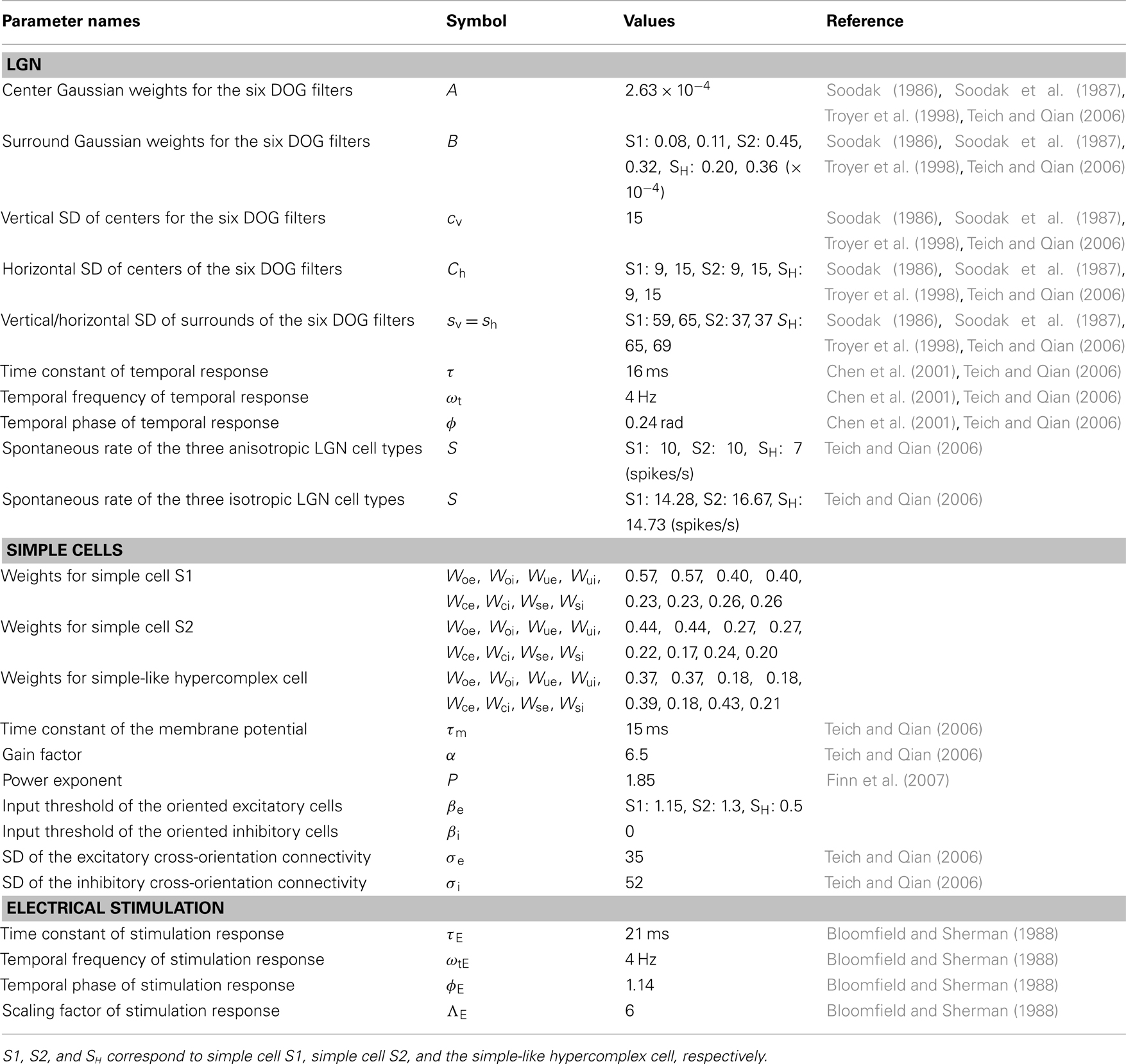
Table 1. Model parameter names, symbols, values, and references.
While it is possible to produce more detailed computational models of the cell types and cortical, laminar and columnar circuitry involved, our philosophy is to first create relatively simple models that include the key features and can explain as much data as possible. The ALD-RM is such a model. Complexity can be increased incrementally to see what new features emerge or new data can be explained based on a given increment in the model.
3 Results
We begin by illustrating the six types of DOG spatial filters implemented for the LGN stage in order to create the simple cells S1 and S2 with length summation and the simple-like hypercomplex cell, SH. Figure 1Bi shows these six types of DOG spatial filters, in two-dimensions and as a one-dimensional plot of the vertical midline of the filter. Simple cell S1 was excited by the anisotropic center with a weak surround (top left) and disynaptically inhibited by the unoriented center with a stronger surround (top right). Simple cell S2 was excited by the anisotropic center with a weak, narrow surround (middle left) and disynaptically inhibited by the unoriented center with a stronger, narrow surround (middle right). A narrower surround was used for simple cell S2, compared to simple cell S1, in order to show similar results can be obtained for different surrounds. The primary difference between simple cells S1 and S2 is that the response of simple cell S2 saturates earlier for shorter bar lengths. This is illustrated in subsequent figures. The simple-like hypercomplex cell with end-stopping (SH) was excited by the anisotropic center with a strong surround (bottom left) and disynaptically inhibited by the isotropic center with a weaker surround (bottom right). Figure 1Bii illustrates that if one considers the cortical RF picture that emerges by subtracting half-wave rectified versions of the unoriented LGN RFs from the half-wave rectified versions of the orientation-biased LGN RFs shown in Figure 1Bi, it is apparent that the cortical RFs look much like even symmetric RFs seen in reverse correlation studies. We refer to the sensitivity profiles in Figure 1Bii as “pseudo-RFs” of the cortical cells because they only partly capture the RF structure of the simulated cells (We revisit this point in the Discussion). If one slightly jittered the spatial positions of the biased and unoriented LGN RFs relative to each other it would also be possible to create cortical pseudo-RFs that begin to look more like those with different spatial phases.
Figures 1Biii,iv demonstrate that the degree of anisotropy of the simulated LGN cell RFs used in this study are realistic by comparing the most orientation-biased response of an ON-center LGN cell simulated in this paper (Figure 1Biii) with real data from an LGN ON-center cell recorded from a cat (Figure 1Biv), data adapted from Vidyasagar and Urbas (1982). Both figures show the response to a light narrow bar. The orientation bias (taken to be the ratio of the response to the preferred orientation and the response to the orthogonal orientation) is 2.34 and 1.95 for the simulated cell and the real cell, respectively. The mean orientation-bias seen in the LGN responses in the cat to narrow bars is 1.99 ± 0.78 for 136 cells (Vidyasagar and Urbas, 1982). The majority of simulated responses showed orientation bias less than that plotted in Figure 1Biii indicating that the biases of our simulated LGN cells are well within the normal range and thus conservative. Shou and Leventhal (1989) applied circular statistics and ellipse fits to polar plots of the responses of 705 cat LGN cells that were stimulated with drifting sinusoidal gratings. They found a mean ellipse axis ratio of 1.27, however, they presented the gratings where the SF was just below the high SF limit of the unit determined for the non-optimal orientation. More recently, for drifting gratings presented at the preferred SF, 41% of 110 LGN cells in the owl monkey showed orientation bias, and the average bias increased with increases in SF for 25 cells investigated (Xu et al., 2002). Xu et al. (2002) however, did not investigate orientation bias at high spatial frequencies for all 110 cells. Vidyasagar and Heide (1984) found for grating stimuli that only 2 of 29 LGN cells showed a significant orientation bias for low spatial frequencies, whereas the vast majority of this sample showed significant orientation bias at high spatial frequencies.
Figure 2 illustrates, using a light-bar stimulus, how the length–response function of a simple cell with length summation can emerge from LGN responses as proposed in the methods. Figures 2A–C correspond to simulations for simple cell S1. Figure 2A plots the length–response functions of an ON LGN field with a vertically biased center and a weak isotropic inhibitory surround, for a vertical bar (solid line) and a horizontal bar (dashed line). Figure 2B plots the length–response functions of an ON LGN field with an isotropic center and a strong isotropic inhibitory surround in response to a vertical bar (solid line) and a horizontal bar (dashed line). Figure 2C plots the length–response functions of simple cell S1 in response to a vertical bar (solid line) and a horizontal bar (dashed line). This cell is simulated to receive excitation from an LGN field as in Figure 2A and inhibition from an LGN field as in Figure 2B. Figure 2D plots the length–response function of a real simple cell with length summation in response to a vertical bar. For the responses to a vertical bar it can be seen that for short bar lengths the input from the biased LGN field to S1 will be inhibited by the unoriented LGN field, but for longer bar lengths the S1 will receive less and less inhibition (i.e., it will be disinhibited). This interaction creates the monotonic length–response function observed for the simple cell with length summation (Rose, 1977). For the responses to a horizontal bar, the disynaptic inhibition by the unoriented LGN field, combined with the recurrent inhibition, nullifies the simple cell response to the bar. Figure 2E plots the length–response functions of simple cell S2 in response to a vertical bar (solid line) and a horizontal bar (dashed line). Simple cell S2 differs from simple cell S1 in that it is influenced by LGN cells with narrower surrounds leading the length–response function of simple cell S2 to saturate at a shorter bar length than is observed for simple cell S1.
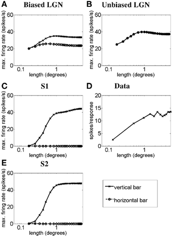
Figure 2. Length–response functions of simple cells S1 and S2 showing length summation. The plots show simulated length–response functions of (A) an ON LGN cell with a vertically biased center and a weak isotropic inhibitory surround, (B) an ON LGN cell with an isotropic center and a strong isotropic inhibitory surround, and (C) the corresponding vertically oriented simple cell S1 in response to a vertical bar (solid lines) and a horizontal bar (dashed lines). (D) The length–response function of a real simple cell with length summation in response to a bar of the preferred orientation (Data adapted from Kato et al., 1978). (E) The response of the vertically oriented simple cell S2 to a vertical bar (solid lines) and a horizontal bar (dashed lines). In (A–C) and (E) the y-axis represents the maximum firing rate (spikes/seconds) reached before the bar is switched off, and the x-axis represents the bar length in degrees. In (D) the y-axis represents number of spikes recorded per response to a bar (as defined by Kato et al., 1978).
Next we simulate the other extreme of simple cell length–response functions. Figure 3 illustrates, using a light-bar stimulus, how the length–response function of a simple-like hypercomplex cell with end-stopping can emerge from LGN responses as proposed in the methods. Figure 3A plots the length–response functions of an ON LGN field with a vertically biased center and a strong isotropic inhibitory surround, for a vertical bar (solid line) and a horizontal bar (dashed line). Figure 3B plots the length–response functions of an ON LGN cell with an isotropic center and a weak isotropic inhibitory surround, again for a vertical bar (solid line) and a horizontal bar (dashed line). Figure 3C plots the length–response functions of the simple-like hypercomplex cell in response to a vertical bar (solid line) and a horizontal bar (dashed line). This cell is simulated to receive excitation from an LGN field as in Figure 3A and inhibition from an LGN field as in Figure 3B. Figure 3D plots the length–response function of a real simple cell with end-stopping in response to a bar of optimum orientation. For the responses to a vertical bar it can be seen that for short bar lengths the biased LGN field’s input to the simple-like hypercomplex cell, SH, will be only slightly inhibited by the unoriented LGN field, but more importantly for longer bar lengths the cortical cell will exhibit significant inhibition. This interaction creates a length–response function with a sharp drop-off in response as bar length increases as is observed for simple-like hypercomplex cells with end-stopping. For the responses to a horizontal bar, the disynaptic inhibition by the unoriented LGN cell, combined with the recurrent inhibition, nullifies the simple cell response to the bar.
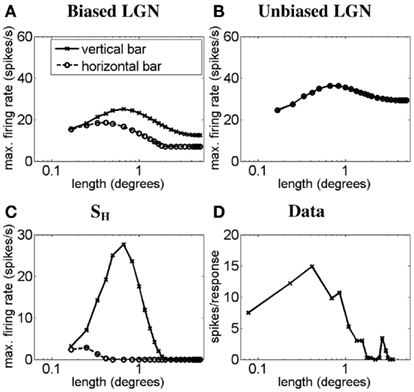
Figure 3. Length–response function of the simple-like hypercomplex cell showing end-stopping. The plots show simulated length–response functions of (A) an ON LGN cell with a vertically biased center and a strong isotropic inhibitory surround, (B) an ON LGN cell with an isotropic center and a weak isotropic inhibitory surround, and (C) the corresponding vertically oriented simple-like hypercomplex cell with end-stopping in response to a vertical bar (solid lines) and a horizontal bar (dashed lines). (D) The length–response function of a real simple-like hypercomplex cell in response to a bar of the preferred orientation (Data adapted from Kato et al., 1978). Axes are the same as defined in Figure 2.
Next we demonstrate for the modeled cell types that we are able to produce realistic SF-response functions in response to gratings and Gabor patches. For the simple cells S1 and S2 with length summation we focus on responses to gratings. For the simple-like hypercomplex cell with end-stopping, full-field gratings did not elicit any response as a result of significant inhibition in the surround. This finding is consistent with recordings from real simple-like hypercomplex cells. Therefore, in place of gratings, we probe the SF response of the simple-like hypercomplex cell using Gabor patches.
In Figure 4 we demonstrate the SF-response functions of simple cell S1 in response to gratings. Similar curves were obtained for simple cell S2 but are not shown here. Figure 4A plots the SF-response functions of an ON LGN cell with a vertically biased center and a weak isotropic inhibitory surround for a vertical grating (solid line) and a horizontal grating (dashed line). Figure 4B plots the SF-response functions of an ON LGN cell with an isotropic center and a strong isotropic inhibitory surround for a vertical grating (solid line) and a horizontal grating (dashed line). Figure 4C plots the SF-response functions of simple cell S1 for a vertical grating (solid line) and a horizontal grating (dashed line). Figure 4D plots the SF-response functions of a real simple cell with length summation to vertical and horizontal gratings. It can be seen that LGN cells generally respond to both low and high spatial frequencies, but the biased LGN cell has a preference for vertical stimuli at higher spatial frequencies. Thus, when the simple cell is excited by the biased field and inhibited by the unoriented field, the simple cell only responds to higher spatial frequencies.
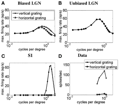
Figure 4. Spatial frequency-response function of the simple cell S1 with length summation. The plots show simulated SF-response functions of (A) an ON LGN cell with a vertically biased center and a weak isotropic inhibitory surround, (B) an ON LGN cell with an isotropic center and a strong isotropic inhibitory surround, and (C) the corresponding vertically oriented simple cell S1 in response to a vertical grating (solid lines) and a horizontal grating (dashed lines). (D) The SF-response function of a real simple cell with length summation in response to vertical and horizontal gratings (Data adapted from Hammond and Pomfrett, 1990). In (A–D) the y-axis represents the maximum firing rate in spikes/seconds, and the x-axis represents the SF in cycles per degree (CPD).
Similar results were obtained for the simple-like hypercomplex cell with end-stopping in response to Gabor patches of different SF. These results are shown in Figure 5. Figure 5A plots the SF-response functions of an ON LGN cell with a vertically biased center and a strong isotropic inhibitory surround for a vertical Gabor patch (solid line) and a horizontal Gabor patch (dashed line). Figure 5B plots the SF-response functions of an ON LGN cell with an isotropic center and a weak isotropic inhibitory surround to a vertical Gabor patch (solid line) and a horizontal Gabor patch (dashed line). Figure 5C plots the SF-response functions of the simple-like hypercomplex cell for a vertical Gabor patch (solid line) and a horizontal Gabor patch (dashed line). Figure 5D plots the SF-response function of a real simple-like hypercomplex cell to a Gabor patch of the preferred orientation. These results are similar to that observed for the simple cell with length summation except that the hypercomplex cell produces a weaker response because of the strong inhibitory surround, especially for longer bars or Gabor patches.
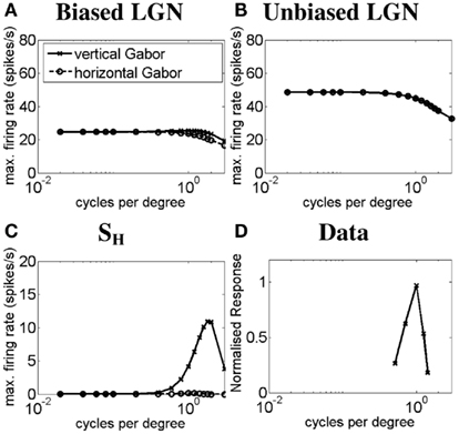
Figure 5. Spatial frequency-response function of the simple-like hypercomplex cell. The plots show simulated SF-response functions of (A) an ON LGN cell with a vertically biased center and a strong isotropic inhibitory surround, (B) an ON LGN cell with an isotropic center and a weak isotropic inhibitory surround, and (C) the corresponding vertically oriented simple-like hypercomplex cell in response to a vertical Gabor patch (solid lines) and a horizontal Gabor patch (dashed lines). (D) The SF-response function of a real simple-like hypercomplex cell in response to a Gabor patch of the preferred orientation (Data adapted from Kulikowski and Bishop, 1981). Axes are the same as in Figure 4 except in (D) the y-axis represents the normalized response to a grating stimulus of limited extent.
Next we demonstrate for the modeled simple cells S1 and S2 and the simple-like hypercomplex cell that we are able to produce realistic OT curves in response to bars, gratings, or Gabor patches. As above we show responses of the simple cells with length summation to gratings and the responses of the simple-like hypercomplex cell to Gabor patches. First we demonstrate how the sharp OT of the cell types emerges. In Figure 6 we consider the simulated OT curve for the case of simple cell S1 in response to a bar 0.5° in length. In Figures 6A–D we see the OT curves of the orientation-biased LGN field driving the simple cell, the unoriented LGN field that disynaptically inhibits the simple cell, the feed-forward input rate received by simple cell S1, and the final response of the simple cell S1, respectively. The feed-forward input rate results from the combination of the excitation and the disynaptic inhibition from LGN. It can be seen that this feed-forward input provides a more tuned input than due to the orientation-biased LGN field alone. Recurrent excitation and inhibition within the cortex then acts to sharpen this input to create a realistic simple cell OT curve. The same mechanisms give rise to OT of simple cell S2 and the simple-like hypercomplex cell, SH.
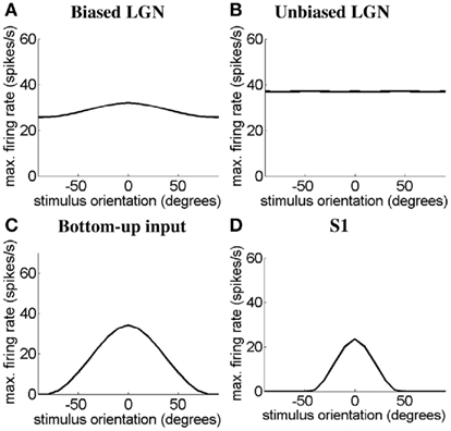
Figure 6. Simulated orientation tuning for simple cell, S1 in response to a bar 0.5° in length. The OT curves are shown for (A) the orientation-biased LGN field with a weak surround driving the simple cell, (B) the unoriented LGN field with a stronger surround that disynaptically inhibits the simple cell, (C) the feed-forward input rate received by the simple cell, and (D) the simple cell S1. In (A–D) the y-axis represents the maximum firing rate in spikes/seconds, and the x-axis represents the bar length in degrees.
In Figure 7 we show the orientation-tuning curves of simple cell S1 (Figure 7A) and the simple-like hypercomplex cell (Figure 7B) in response to bars of different length (see legend in Figure 7). These OT curves are compared to those of a real simple cell without end-stopping (Figure 7C) and a real simple-like hypercomplex cell (Figure 7D) in response to bars of different lengths. It can be seen for the model cells that as bar length increases OT sharpens, as is observed in the real cells. The same effect was observed for simple cell S2, but it is not shown here.
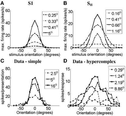
Figure 7. Orientation-tuning curves of (A) the simulated simple cell S1, (B) the simulated simple-like hypercomplex cell, (C) a real simple cell with length summation (data adapted from Rose, 1977), and (D) a real simple-like hypercomplex cell (data adapted from Orban et al., 1979) in response to bars of different lengths. Axes the same as in Figure 6.
Figure 8 demonstrates the orientation-tuning curves of simple cell S2 in response to gratings of different spatial frequencies (Figure 8A) and the simple-like hypercomplex cell in response to Gabor patches of different SFs (Figure 8B). These OT curves are compared to those of a real simple cell without end-stopping in response to gratings of different SFs (Figure 8C). It can be seen for the model cells that as SF increases OT sharpens, as is observed in the real cell. Simple cell S1 produced slightly different OT curves to that seen for simple cell S2 here. However, as is illustrated in Figures 9B,D, it turns out that the plots of half-width-at-half-height (HWHH) versus SF for the simple cells S1 and S2 and the simple-like hypercomplex cell SH still correspond closely to those observed for real simple cells. Of further note, there is flexibility with parameters in that the HWHH versus SF curve obtained for simple cell S1 could look more like that obtained for simple cell S2 depending on how parameters are selected (simulations not shown). Figures 9A,C plot HWHH versus bar length for the simulated cells and for real cells, respectively. It can be seen that for the simple cells with length summation the HWHH versus bar length curve flattens out, whereas for the simple-like hypercomplex cell it decreases until the cell no longer responds to bars of increasing length.
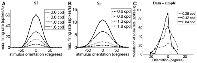
Figure 8. Orientation-tuning curves of (A) the simulated simple cell S2 and (C) a real simple cell with length summation (data adapted from Vidyasagar and Siguenza, 1985) in response to gratings of different SFs. (B) OT curves of the simulated simple-like hypercomplex cell in response to Gabor patches of different SFs. Legends indicate the SF in cpd. In each plot the y-axis represents the maximum firing rate in spikes/seconds, and the x-axis represents the orientation of the grating or Gabor patch stimulus in degrees.
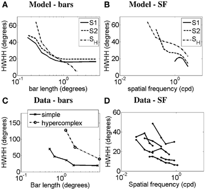
Figure 9. Half-width-at-half-height (HWHH) versus bar length and HWHH versus spatial frequency. HWHH versus bar length curves produced by (A) the model and (C) real simple cells in response to bars (Data adapted from Henry et al., 1974 and Orban et al., 1979). In (A,C) the y-axis represents the HWHH in degrees, and the x-axis represents the bar length in degrees. HWHH versus SF curves produced by (B) the model in response to gratings and Gabor patches and (D) real simple cells in response to gratings (Data adapted from Vidyasagar and Siguenza, 1985). In (B,D) the y-axis represents the HWHH in degrees, and the x-axis represents the SF in cpd. Legend – S1: simple cell S1, S2: simple cell S2, SH: simple-like hypercomplex cell.
Next, we simulate the effects of iontophoretic application of bicuculline, a GABAA antagonist, on length response, SF tuning, and OT curves (Sillito, 1975; Tsumoto et al., 1979; Vidyasagar, 1984b; Vidyasagar and Mueller, 1994). To do this we simulated the effect of bicuculline by reducing the inhibitory weights connecting to the cell of interest by multiplying them by the factor Λ = 0.1.
Figure 10 shows the simulation results for the effects of bicuculline. Figures 10A,E plot the length–response functions of simple cell S1 and a real simple cell with length summation, respectively. It can be seen that the release from inhibition by bicuculline injection causes the simple cell to reveal a length–response function much like that of the orientation-biased LGN field that is driving it (see Figure 2A), with all the length summation occurring within a shorter length. In our scheme this is due to the reduced inhibition for bars of longer length due to the strong surround of the LGN field that provides the disynaptic inhibition. Figures 10B,F plot the length–response functions of a simulated simple-like hypercomplex cell and a real simple-like hypercomplex cell, respectively. Again the length–response function in the bicuculline case is similar to the length–response function of the LGN cell that is driving it (see Figure 3A). Figures 10C,G plot the SF-response functions of simple cell S2 and a real simple cell with length summation, respectively. It can be seen that blockade of inhibition causes a broadening of the SF response function. Figures 10D,H plot the OT curves for the simulated simple cell S2 and a real simple cell, respectively. Here it can be seen that blockade of inhibition causes broadening of the OT curve. Similar results to those shown in Figure 10 were observed for all other cell types and stimulus-type combinations not shown in the figure.
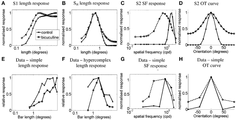
Figure 10. Effects of iontophoretic application of bicuculline. (A,E) plot the length–response functions of simple cell S1 and a real simple cell with length summation (Data adapted from Vidyasagar, 1984b) for a bar stimulus of the preferred orientation, respectively. (B,F) plot the length–response functions of a simulated simple-like hypercomplex cell and a real simple-like hypercomplex cell (Data adapted from Vidyasagar, 1984b) for a bar stimulus of the preferred orientation, respectively. (C,G) plot the SF-response functions of simple cell S2 and a real simple cell with length summation (Data adapted from Vidyasagar and Mueller, 1994) for a grating stimulus of the preferred orientation, respectively. (D,H) plot the OT curves for the simulated simple cell S2 for a bar length 1.66° and a real simple cell (Data adapted from Tsumoto et al., 1979), respectively. Control responses are indicated by solid lines, while responses under the influence of bicuculline are indicated by dashed lines.
Changes in cortical orientation tuning can potentially happen also in many experimental situations other than bicuculline application, which manipulate the inputs to a striate cell. One recent instance of this is a study that applied electrical stimulation in the LGN while recording from the striate cortex (Kara et al., 2002). Their rationale was to suppress all cortical activity through the strong intra-cortical inhibition evoked by the stimulation and thus be able to study the “raw” feed-forward inputs from the LGN alone. More recently, Viswanathan et al. (2011), used a variation of Kara et al.’s original paradigm and recorded from both striate cortex and the LGN during electrical stimulation in the LGN at a rate of around 7.75 Hz. They found that orientation sensitivity of LGN cells was significantly sharpened during the stimulation and also that there was some reduction of orientation selectivity of layer 4 cortical cells. Figure 11 provides a simulation of these results. Figures 11G,H show polar response plots of a real LGN cell and a real simple cell, respectively, during either visual stimulation with bars (solid line) or both visual stimulation and electrical stimulation of the LGN (dashed line). Figures 11A–F show a simulation of this kind of data for the S1 simple cell which has had its baseline tuning set to a broader value by lowering the threshold of the excitatory oriented cortical cells, βe, from 1.15 to 0. To compensate for the lower threshold the feed-forward weights were also lowered to the following values: Woe = Woi = 0.34, Wue = Wui = 0.24. This modified S1 simple cell is referred to here as S1*. Figures 11A,B show the responses of the orientation-biased LGN cell that excites, and the unoriented LGN cell that inhibits, the simple cell S1*, respectively. It can be seen that electrical stimulation of the LGN reduces the response of the LGN to bars and at the same time sharpens the tuning of the orientation-biased LGN cell to a similar extent to the real data in Figure 11G. This occurs as a result of a “tip of the iceberg” effect due the strong degree of suppression introduced by electrical stimulations. Figures 11C,D show the responses of the feed-forward inputs to, and the outputs of, the S1* simple cell, respectively. It can be seen that the feed-forward tuning is both reduced and broadened as a result of electrical stimulation, while the output of the S1* simple cell is reduced and only slightly broadened. The S1* output response is only slightly broadened due to the strong effects of the power-law and intra-cortical interactions.
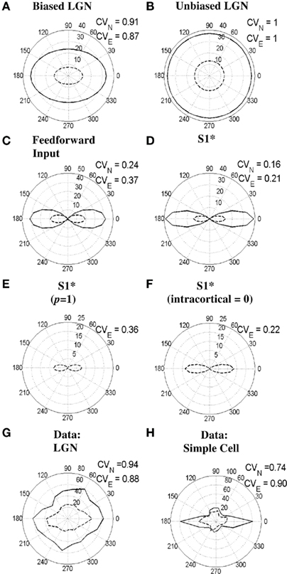
Figure 11. Effects of electrical stimulation in the LGN on orientation selectivity of LGN and simple cells. (A–F) show simulations for the simple cell S1* (see text) in response to bars of length 4.17° either without or during electrical stimulation of the LGN. (A,B) show the responses of the orientation-biased and unoriented LGN cells that provide the feed-forward input to the simple cell, respectively. (C,D) show the responses of the combined feed-forward input to, and the output of, the S1* simple cell, respectively. (E,F) illustrate the output of the S1* simple cell when either the power-law exponent is reduced to p = 1 (from 1.85) or the intra-cortical input is set to zero (i.e., Wce = Wci = Wse = Wsi = 0), respectively. (G,H) demonstrate the responses of a real LGN cell and a real simple cell to bars, respectively, both with or without electrical stimulation in the LGN (adapted from Viswanathan et al., 2011). In all subfigures, responses to visual stimulation alone are indicated by the solid lines, whereas responses to visual stimulation during electrical stimulation are indicated by the dashed lines. Moreover, the CVN and CVE values next to each subfigure indicate the circular variance values calculated from the responses to normal visual stimulation alone or visual stimulation during electrical stimulation, respectively.
To explore the role these model components play during electrical stimulation, the power-law was removed (by reducing the power-law exponent to p = 1) or the intra-cortical input was set to zero (i.e., Wce = Wci = Wse = Wsi = 0) in Figures 11E,F, respectively. During electrical stimulation cortex appears to operate in a predominantly subthreshold regime in between stimulation pulses. This regime may reduce the influence of intracellular excitatory feedback mechanisms (Pei et al., 1994) when a probing pulse arrives and therefore it is reasonable to assume electrical stimulation results in a reduced power-law exponent. This idea is consistent with the simulations where CV increases from 0.16 for the normal response of the S1* cell (Figure 11D) to 0.36 for the S1* cell with p = 1 (Figure 11E) when electrical stimulation is introduced. This magnitude change of 0.20 is consistent with the real simple cell data in Figure 11H where CV increases by 0.16 from 0.74 to 0.90 when electrical stimulation is introduced. Given that cortex is largely silenced during electrical stimulation of the LGN it is also reasonable to assume that the intra-cortical input to a cell could become negligible (Kara et al., 2002). This is assumed in Figure 11F, however, it is apparent that for the set of parameters defining S1* and the stimuli used, the intra-cortical input does not greatly affect the orientation selectivity when compared to Figure 11D.
The discrepancy in CV values for the simple cell data in Figure 11H and the S1* simulations in Figures 11D–F result from the fact that the real cell is more broadly tuned than the model cell. This is primarily because we sought to make the simplest modification to the S1 simple cell that would create a significant reduction in tuning during electrical stimulation. Prior to modification, the S1 simple cell was sharply tuned and so did not show significant increases in CV with electrical stimulation of the LGN. Similar broadening of the cortical tuning width is also seen in the data of Kara et al. (2002), even though the change did not reach statistical significance, possibly due to the small sample size (n = 6).
Generally, in our model, electrical stimulation of the LGN appears to result in broadening of the cortical response by weakly activating cells tuned to all orientations at the times of electrical stimulation. This broadening can be further enhanced by reducing the power-law exponent as described above. However, there is a trade-off between this broadening effect and the fact that increasing the strength of electrical stimulation further sharpens the selectivity of the orientation-biased LGN input which in turn should sharpen the cortical response. This trade-off depends on the values of the parameters used.
Vidyasagar (1985, 1987) has proposed that similar to the way color is coded as a combination of activities in separate broadly tuned channels, it may be possible to code also for orientation by creating a simple cell tuned to an arbitrary orientation from a combination of LGN cells tuned to cardinal orientations. This possibility is supported by evidence that the distribution of preferred orientations of cells showing orientation selectivity in the cat retina (Hammond, 1974; Levick and Thibos, 1980; Leventhal and Schall, 1983; Schall and Leventhal, 1987), rat retina (Schall et al., 1987), ferret retina (Vitek et al., 1985), macaque retina (Schall et al., 1986), and cat LGN (Vidyasagar and Urbas, 1982; Shou and Leventhal, 1989) demonstrate an overrepresentation of a few orientations, in particular the horizontal, the vertical or the radial (“radial” being along the line joining the center of area centralis or fovea to the ganglion cell location). Thus if subcortical orientation selectivity is critical for cortical selectivity for this parameter, it is coded precisely in the way that color is coded – i.e., in a limited number of broadly tuned channels so as not to forsake resolution and sensitivity for the sake of discrimination. This tendency for overrepresentation of a few cardinal orientations is also reflected in the striate (Leventhal, 1983; Li et al., 2003) and extrastriate (Leventhal et al., 1984) areas of the cat and in the ferret striate cortex (Chapman and Bonhoeffer, 1998; Coppola et al., 1998; Grabska-Barwinska et al., 2009). Given that most orientations are represented at each retinotopic coordinate in the LGN, cortical cells could either be driven by orientation-biased LGN cells with the same orientation preference as the cortical cell or by a combination of signals tuned optimally to different cardinal orientations or both.
Here we present a proof-of-concept simulation of such a “cardinal” construction of cortical orientation tuning. For three or four cardinal orientations it is straightforward with our model to create all orientations. For only two cardinal orientations, say vertical and horizontal, at a first glance there appears to be difficulty in resolving the orientation of oblique orientations symmetric about one or the other cardinal axes, but this ambiguity can be resolved by modeling LGN cells as having both an orientation bias and a direction bias. Such direction bias has also been observed in vivo for LGN cells (e.g., see figures in Vidyasagar and Urbas, 1982; Xu et al., 2002). Introduction of a direction bias and providing a simulation with only two cardinal orientations can be done by modifying our present model to make the LGN or their input retinal cells at least weakly direction selective, as for example in Reichardt (1969) detectors.
Instead, here in Figure 12 we show a simulation of the simple cell type S1, where the orientation tuning of cortical cells over the full range of orientations can be produced by linear combination of LGN RFs with only four distinct orientation biases. We chose to simulate four orientation biases equally spaced within 180° as this includes the vertical and horizontal biases of LGN cells seen often in the data. The simulation of simple cell S1 was modified such that only 4 LGN orientation biases are encoded, as opposed to 18. A given simple cell orientation preference was determined by a linear combination of the four LGN orientation-biased cell outputs. The linear combination weights of the orientation-biased LGN cells were determined using an optimization method such that feed-forward tuning curves look like the feed-forward tuning of the original S1 cell.
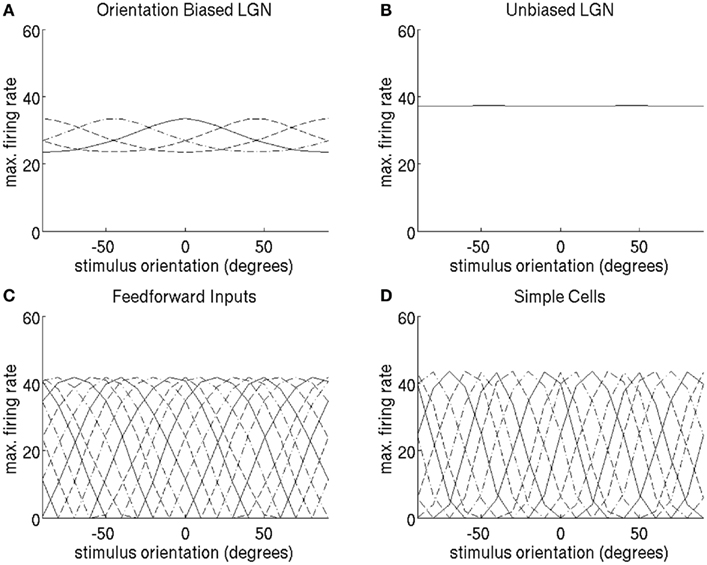
Figure 12. “Cardinal” construction of 18 simple cell orientation-tuning curves tuned to the full range of orientation preferences by linearly combining orientation-biased LGN cells with only four orientation biases. Orientation-tuning curves were obtained by stimulating with a bar of length 4.16°. (A) The orientation-tuning curves of the four LGN cells with orientation bias. The unoriented LGN response in (B) was subtracted from a linear combination of the orientation-biased LGN cells to produce the orientation-tuning curves of the feed-forward input to the simple cells in (C). (D) The tuning curves of the simple cells obtained after recurrent competition. For the sake of clarity, tuning curves alternate between solid, dashed, and dash-dot lines.
4 Discussion
4.1 Mechanisms of Orientation Selectivity of Simple Cells
Here we have presented a model describing how the orientation-bias of a single LGN field can help to create OT, SF, and length–response properties of simple and simple-like hypercomplex cells. Although additional mechanisms such as excitatory convergence (Hubel and Wiesel, 1962; Wörgötter and Koch, 1991; Reid and Alonso, 1995; Finn et al., 2007), projection of spatially offset ON and OFF LGN cells (Schiller, 1982; Sherk and Horton, 1984; Hirsch, 2003), or opponent inhibition (Troyer et al., 1998, 2002; Hirsch, 2003; Hirsch et al., 2003) are likely to influence the response properties of simple cells we have presented the simplest model involving LGN orientation bias in a single LGN field required to explain the data of interest. This model involved excitation of a simple cell by an anisotropic LGN field and disynaptic inhibition by an unoriented LGN field combined with recurrent excitation and inhibition between oriented simple cells. The oriented LGN field gives untuned responses at low spatial frequencies but greater tuning to preferred orientations for higher spatial frequencies. Subsequent disynaptic inhibition in the cortex effectively removes the response to the low spatial frequencies leaving only the response to preferred orientations at high spatial frequencies. Recurrent cortical excitation and inhibition then acts to further sharpen OT. Evidence exists for both the oriented and unoriented or weakly oriented inhibitory cells implemented in the model. Specifically, inhibitory cells in layer 4 were either of the oriented type (Hirsch et al., 2003) or showing only weak orientation biases (Hirsch et al., 2003; Nowak et al., 2008).
We have also shown that experimental manipulations that alter the balance between excitation and inhibition, in either the input to the cortex or intracortically, or at both sites, can be simulated in our model. Changes in response properties of LGN and striate cells brought about by either iontophoretic application of bicuculline near cortical cells or electrical stimulation in the LGN were successfully simulated. The results of the electrical stimulation studies can potentially also be the basis for more detailed modeling using spiking neurons to test potential underlying mechanisms.
For the sake of parsimony, in our simulations we have focused on simulating only ON LGN cells, but our simulations are consistent with evidence for the projection of both ON and OFF cells to a single simple cell (Sherk and Horton, 1984; Hirsch, 2003). Just as an ON anisotropic LGN cell excites the simple cell and an ON isotropic LGN cell disynaptically inhibits a simple cell in the model, it is also possible for an OFF anisotropic LGN cell and an OFF isotropic cell to do the same. The phase variation of the ON/OFF envelope (DeAngelis et al., 1995) could also be included in the model through greater consideration of the temporal properties of ON and OFF cells.
Hebbian learning, or spike-timing-dependent-plasticity (STDP; Song et al., 2000; Bartsch and van Hemmen, 2001) mechanisms could help to ensure that these ON and OFF projections do not coincide with the same spatial co-ordinate, but instead spatially adjacent co-ordinates. This is expected since light never spatially correlates with dark in natural images. It is also possible to create oriented simple cells of all different spatial phases by combining at least 2, and not necessarily many more, spatially offset ON and OFF cells along the spatial axis orthogonal to the preferred orientation-bias of the ON and OFF LGN cells.
That being said, Hebbian learning is also likely to support the formation of excitatory convergence. For example, spatially offset anisotropic ON LGN cells aligned along the axis of their preferred orientation are likely to be correlated when activated by light edges and thus connect to the same simple cell. This would lead to an excitatory convergence as originally proposed by Hubel and Wiesel (1962). This is also supported by the elongated clustering of LGN afferents seen within orientation columns of the ferret (Chapman et al., 1991) and the regular alignment of LGN ON and OFF fields seen in cat simple cell subregions (Reid and Alonso, 1995; Alonso et al., 2001; Jin et al., 2011). However these studies do not provide a satisfactory explanation for their own observation and those of others (Henry et al., 1978; Bullier et al., 1982; Pei et al., 1994) that the aspect ratios of simple cell RFs obtained from two-dimensional noise stimuli or short bars are much shorter than the region of apparent excitatory facilitation seen in length–response functions. Our model not only explains this through the disinhibition along the length axis discussed earlier under Results, but also shows that orientation bias of LGN cells can reduce the need for excitatory convergence. In particular, orientation-bias of a single LGN cell can then be expected to play a significant role in the central visual field where excitatory convergence needs to be minimized to provide a high resolution representation of the visual scene. Moreover, as pointed out by Ringach (2011), Jin et al. (2011) recent findings suggest substantial constraint of the cortical cells’ inputs by asymmetries in LGN RFs.
The above discussion also relates to the problem of why simple cell RFs can appear longer than LGN RFs. As observed in our simulations of simple cells without end-stopping, disinhibition of the anisotropic LGN RF by the isotropic LGN RF for longer bars shows that our ALD-RM simple cell can uniquely encode bar length, not just to the edge of the centers of the LGN RFs but to the very edge of the LGN RF surround. This indicates that length summation properties (thought to be reflective of “larger” RFs) can occur by a mechanism other than just excitatory convergence. As can be seen in Figure 2C, the response of the simulated cell S1 increases with increasing bar length up to 5°, whereas the green excitatory region in the S1 pseudo RF in Figure 1Bii extends only over 1°. This indicates that the pseudo-RFs are only a partial description of the simulated cells’ response function.
Another key question one might have regarding whether orientation-bias of single LGN cells can really have an influence on simple cell OT is: how can the oriented LGN cells produce the full range of orientations seen in primary visual cortex? As mentioned in the results (Figure 12), Vidyasagar (1985, 1987) has proposed a possible solution to this question, by coding for orientation by creating a simple cell tuned to an arbitrary orientation from a combination of LGN cells biased toward cardinal orientations. If the full range of cortical orientation preferences are thus built from the inputs from a limited number of subcortical channels, one can expect this to be reflected in the distribution of preferred orientations in the striate cortex. Such a bias toward cardinal orientations is in fact observed in both single cell (Leventhal, 1983; Li et al., 2003) and optical imaging (Chapman and Bonhoeffer, 1998; Coppola et al., 1998; Wang et al., 2003) studies of the primary visual cortex. At the same time, there is the possibility that construction of non-cardinal orientations from cardinal orientations may not be necessary if there is a precise match of orientation distributions among cortical simple cells and the orientation distributions in the retina at the same retinotopic co-ordinate as at least one study suggests (Schall et al., 1986). Our model is consistent with such a match between cortical and retinal distributions of preferred orientations. In any case, it is unclear how the excitatory convergence model ala Hubel and Wiesel can account for the presence of radial biases in the cortical data, given that their model assumes isotropy of the LGN responses. Aligned convergence of afferents would have to somehow respect the location specific orientation distributions seen in the retina and LGN while actually ignoring the same biases in generating orientation sensitivity. Furthermore such developmental consideration has also to be valid across a number of different species.
The emergence of the full range of orientations from a limited number of broadly tuned input channels can also form the framework for the known columnar architecture of the cortex (Vidyasagar et al., 1996). A full simulation of that is in progress, but it is beyond the scope of the present paper. An additional simple cell property that we have not simulated here is direction selectivity. In the same way that biases to (cardinal) orientations among LGN cells can construct sharp orientation selectivity in cortical simple cells with their optimal orientations distributed across the full range, biases to (cardinal) directions in the LGN can construct a range of direction selectivities in simple cells. Moreover, as hinted at in the second last paragraph of the results, the combination of bias to (cardinal) orientations and (cardinal) directions in the LGN could be used to construct a combined coding of a full range of orientation and direction selectivities among simple cells.
4.2 Comparison to Other Computational Models
In our simulations, we have applied a power-law spike-rate response function and recurrent excitation and inhibition to sharpen the OT of simple cells. We were also able to obtain similar results (not shown here) if we still allowed for excitation of a simple cell by an anisotropic LGN cell and disynaptic inhibition by an isotropic LGN cell, but combined these features with only thresholding and a power-law spike-rate response function. However, this required much higher thresholds and had less flexibility in obtaining the desired responses than were able to be obtained with cross-orientation excitation and inhibition. Finn et al. (2007) employed a thresholding and power-law transfer function mechanism to explain contrast invariance in simple cells without needing a dependence on cross-orientation inhibition. The input to their model followed the excitatory convergence model, consisting of spatially aligned unoriented LGN cells. Although more local, the alternative bottom-up input we have proposed would still provide a similar description of OT and contrast invariance. Similarly, contrast invariance demonstrated for models based on the combination of excitatory convergence and recurrent excitation and inhibition (i.e., the RM; Somers et al., 1995; Teich and Qian, 2006) would still be present if simulations were done with our alternative input.
Teich and Qian (2006) compared simulations of the RM involving oriented cells of only one spatial phase (single-phase RM) and the RM involving oriented cells with different spatial phases (multi-phase RM). For the sake of simplicity we have effectively simulated a single-phase RM (with different bottom-up inputs), but our results would still hold for the multi-phase RM. Teich and Qian (2006) suggested that the multi-phase RM is a model for complex cells and that it needs to be modified to include opponent inhibition to provide a description of simple cells. We found that our version of the single-phase RM presented here still provides a good description of simple cells. This is not only based on the response properties investigated but we also found that F1/F0 ratios (Movshon et al., 1978a,b, 2006) for the simulated simple cells were always greater than 1. This makes sense as our version of the single-phase RM is not influenced by stimuli of any phase other than the cell’s preferred phase.
With regard to model complexity we have sought to present a simple rate-based neuron network to explain the properties of interest. The degree of model complexity is similar to that employed by Teich and Qian (2006) who compared the RM (Somers et al., 1995) and the modified feed-forward model (MFM; Troyer et al., 1998), and a hybridization of the two. All of these models relied on excitatory convergence in the input. Some models have considered spiking neurons (Somers et al., 1995) but the complexities associated with compartmental neurons are often ignored. Models that consider networks in more detail are often rate-based and aim to describe properties of orientation selectivity, and orientation and ocular dominance columns (Erwin and Miller, 1998; Kayser and Miller, 2002). Often these models do not include the laminar circuits of cortex which are likely to be important for modeling the true circuitry of various mechanisms, such as cross-orientation interactions. Here and in other models, cross-orientation mechanisms are modeled with the functional idea of Mexican hat cross-orientation excitation and inhibition because the true underlying circuitry is not well understood. In this context our model represents a stepping stone for considering models with more detailed cell types and anatomical circuitry.
The main advantage of our ALD-RM model is that it considers the orientation bias of LGN cells. No other model does this, since all computational models of cortical simple cells to date had assumed that the LGN RFs are isotropic. We have based our model on the orientation biases of LGN cells and their dependence on the SF of the stimulus and also the length–response functions of LGN cells. In doing so, not just orientation selectivity of cortical simple cells, but also SF and length selectivities of cortical cells simply fall out of the model. To further understand how the LGN orientation bias specifically contributes to orientation selectivity of simple cells, Figures 6C and 11C give a feel for the orientation selectivity produced by the combination of feed-forward excitation by a biased LGN field and inhibition by an unbiased LGN field. Comparing these Figures to Figures 6D and 11D illustrates the additional influence cross-orientation mechanisms (Somers et al., 1995) and the power-law transfer function (Finn et al., 2007) have on the orientation selectivity of the simple cell. It can be seen that the orientation selectivity of the feed-forward LGN input is quite strong, thus requiring less influence from the other mechanisms. However, the other mechanisms could be made more influential by changing the parameters. The key data that the power-law and the cross-orientation mechanisms cannot explain on their own are the SF and length–response properties which depend largely on the feed-forward LGN input used in our model. The combination of excitatory convergence with the power-law and cross-orientation mechanisms can explain the SF data, but would require additional cortical spatial competition to describe length–response data. The same can be said of current models that combine excitatory convergence and opponent inhibition (Troyer et al., 1998), although opponent inhibition could be designed such that it has similar effects on length–response properties as the excitatory and inhibitory LGN fields have in our ALD-RM model.
Our model is the first to simulate the LGN stimulation experiments of Viswanathan et al. (2011). The only simulations that consider electrical stimulation in the retina or the LGN are related to retinal prostheses, but they assume unbiased retinal RFs (Greenberg et al., 1999). Models to simulate blockade of GABAA include studies on the striate cortex by Somers et al. (1995) and Troyer et al. (1998). Models that combine excitatory convergence and cross-orientation mechanisms (Somers et al., 1995) or opponent inhibition (Troyer et al., 1998) can explain the effects of GABAA blockade on orientation selectivity, but such models do not explain the effects of GABAA blockade on length–response functions because they were not designed to do so. Our model is able to achieve this because it does not ignore the known length–response properties of the LGN fields that excite and inhibit the simple cell. No additional, undocumented, cortical mechanisms are necessary to explain this property.
5 Conclusion
We have shown that a parsimonious computational model of simple and simple-like hypercomplex cells receiving excitatory feed-forward input from only a single orientation-biased LGN field and inhibitory input from another LGN field, can describe their orientation, SF and length–response functions, without assuming any spatially aligned convergence of LGN RFs. This has wider implications for the formation of orientation and ocular dominance columns and the representation of the visual scene in primary visual cortex.
Conflict of Interest Statement
The authors declare that the research was conducted in the absence of any commercial or financial relationships that could be construed as a potential conflict of interest.
Acknowledgments
We thank Jaikaishan Jayakumar and Sivaram Viswanathan for helpful discussions. This work was supported by an Australian Research Council Discovery Grant to Trichur R. Vidyasagar (DP0986247).
References
Allison, J. D., Smith, K. R., and Bonds, A. B. (2001). Temporal-frequency tuning of cross-orientation suppression in the cat striate cortex. Vis. Neurosci. 18, 941–948.
Alonso, J. M., Usrey, W. M., and Reid, R. C. (2001). Rules of connectivity between geniculate cells and simple cells in cat primary visual cortex. J. Neurosci. 21, 4002–4015.
Bartsch, A. P., and van Hemmen, J. L. (2001). Combined Hebbian development of geniculocortical and lateral connectivity in a model of primary visual cortex. Biol. Cybern. 84, 41–55.
Berman, N. J., Douglas, R. J., Martin, K. A., and Whitteridge, D. (1991). Mechanisms of inhibition in cat visual cortex. J. Physiol. (Lond.) 440, 697–722.
Bloomfield, S. A., and Sherman, S. M. (1988). Postsynaptic potentials recorded in neurons of the cat’s lateral geniculate nucleus following electrical stimulation of the optic chiasm. J. Neurophysiol. 60, 1924–1945.
Bonds, A. B. (1989). Role of inhibition in the specification of orientation selectivity of cells in the cat striate cortex. Vis. Neurosci. 2, 41–55.
Bullier, J., Mustari, M. J., and Henry, G. H. (1982). Receptive-field transformations between LGN neurons and S-cells of cat striate cortex. J. Neurophysiol. 47, 417–438.
Buzás, P., Kovács, K., Ferecskó, A. S., Budd, J. M., Eysel, U. T., and Kisvárday, Z. F. (2006). Model-based analysis of excitatory lateral connections in the visual cortex. J. Comp. Neurol. 499, 861–881.
Carandini, M., and Ringach, D. L. (1997). Predictions of a recurrent model of orientation selectivity. Vision Res. 37, 3061–3071.
Chapman, B., and Bonhoeffer, T. (1998). Overrepresentation of horizontal and vertical orientation preferences in developing ferret area 17. Proc. Natl. Acad. Sci. U.S.A. 95, 2609–2614.
Chapman, B., Zahs, K. R., and Stryker, M. P. (1991). Relation of cortical cell orientation selectivity to alignment of receptive fields of geniculocortical afferents that arborise within a single orientation column in ferret visual cortex. J. Neurosci. 11, 1347–1358.
Chen, Y., Wang, Y., and Qian, N. (2001). Modeling V1 disparity tuning to time-varying stimuli. J. Neurophysiol. 86, 143–155.
Chung, S., and Ferster, D. (1998). Strength and orientation tuning of the thalamic input to simple cells revealed by electrically evoked cortical suppression. Neuron 20, 1177–1189.
Cleland, B. G., Lee, B. B., and Vidyasagar, T. R. (1983). Response of neurons in the cat’s lateral geniculate nucleus to moving bars of different length. J. Neurosci. 3, 108–116.
Coppola, D. M., White, L. E., Fitzpatrick, D., and Purves, D. (1998). Unequal representation of cardinal and oblique contours in ferret visual cortex. Proc. Natl. Acad. Sci. U.S.A. 95, 2621–2623.
Creutzfeldt, O., and Ito, M. (1968). Functional synaptic organization of primary visual cortex neurones in the cat. Exp. Brain Res. 6, 324–352.
Creutzfeldt, O. D., Kuhnt, U., and Benevento, L. A. (1974). An intracellular analysis of visual cortical neurones to moving stimuli: response in a co-operative neuronal network. Exp. Brain Res. 21, 251–274.
Crook, J. M., Kisvárday, Z. F., and Eysel, U. T. (1998). Evidence for a contribution of lateral inhibition to orientation tuning and direction selectivity in cat visual cortex: reversible inactivation of functionally characterized sites combined with neuroanatomical tracing techniques. Eur. J. Neurosci. 10, 2056–2075.
da Costa, N. M., and Martin, K. A. (2009). The proportion of synapses formed by the axons of the lateral geniculate nucleus in layer 4 of area 17 of the cat. J. Comp. Neurol. 516, 264–276.
DeAngelis, G. C., Ozhawa, I., and Freeman, R. D. (1995). Receptive field dynamics in the central visual pathways. Trends Neurosci. 18, 451–458.
Douglas, R. J., Martin, K. A., and Whitteridge, D. (1991). An intracellular analysis of the visual responses of neurones in cat visual cortex. J. Physiol. (Lond.) 440, 659–696.
Erwin, E., and Miller, K. D. (1998). Correlation-based development of ocularly-matched orientation and ocular dominance maps: determination of required input activities. J. Neurosci. 18, 9870–9895.
Ferster, D. (1986). Orientation selectivity of synaptic potentials in neurons of cat primary visual cortex. J. Neurosci. 6, 1284–1301.
Ferster, D., Chung, S., and Wheat, H. (1996). Orientation selectivity of thalamic input to simple cells of cat visual cortex. Nature 380, 249–252.
Ferster, D., and Miller, K. D. (2000). Neural mechanisms of orientation selectivity in the visual cortex. Ann. Rev. Neurosci. 23, 441–471.
Finn, I. M., Priebe, N. J., and Ferster, D. (2007). The emergence of contrast-invariant orientation tuning in simple cells of cat visual cortex. Neuron 54, 137–152.
Friedlander, M. J., Lin, C. S., Stanford, L. R., and Sherman, S. M. (1981). Morphology of functionally identified neurons in lateral geniculate nucleus of the cat. J. Neurophysiol. 46, 80–129.
Grabska-Barwinska, A., Distler, C., Hoffmann, K. P., and Jancke, D. (2009). Contrast dependence of cardinal preference: stable oblique effect in orientation maps of ferret visual cortex. Eur. J. Neurosci. 29, 1258–1270.
Greenberg, R. J., Velte, T. J., Humayun, M. S., Scarlatis, G. N., and de Juan, E. Jr. (1999). A computational model of electrical stimulation of the retinal ganglion cell. IEEE Trans. Biomed. Eng. 46, 505–514.
Grossberg, S., and Mingolla, E. (1985). Neural dynamics of form perception: boundary completion, illusory figures and neon color spreading. Psychol. Rev. 92, 173–211.
Hammond, P. (1974). Cat retinal ganglion cells: size and shape of receptive field centres. J. Physiol. (Lond.) 242, 99–118.
Hammond, P., and Pomfrett, C. J. D. (1990). Influence of spatial frequency on tuning and bias for orientation and direction in the cat’s striate cortex. Vision Res. 30, 359–369.
Heggelund, P. (1981). Receptive field organization of simple cells in cat striate cortex. Exp. Brain Res. 42, 89–98.
Henry, G. H., Bishop, P. O., and Dreher, B. (1974). Orientation axis and direction as stimulus parameters for striate cells. Vision Res. 14, 767–777.
Henry, G. H., Goodwin, A. W., and Bishop, P. O. (1978). Spatial summation of responses in receptive fields of single cells in cat striate cortex. Exp. Brain Res. 32, 245–266.
Hirsch, J. A. (2003). Synaptic physiology and receptive field structure in the early visual pathway of the cat. Cereb. Cortex 13, 63–69.
Hirsch, J. A., Martinez, L. M., Pillai, C., Alonso, J. M., Wang, Q., and Sommer, F. T. (2003). Functionally distinct inhibitory neurons at the first stage of visual cortical processing. Nat. Neurosci. 6, 1300–1308.
Hubel, D. H., and Wiesel, T. N. (1962). Receptive fields, binocular interaction and functional architecture in the cat’s visual cortex. J. Physiol. (Lond.) 160, 106–154.
Hubel, D. H., and Wiesel, T. N. (1968). Receptive fields and functional architecture of monkey striate cortex. J. Physiol. (Lond.) 195, 215–243.
Jin, J., Wang, Y., Swadlow, H. A., and Alonso, J. M. (2011). Population receptive fields of ON and OFF thalamic inputs to an orientation column in visual cortex. Nat. Neurosci. 14, 232–240.
Kara, P., Pezaris, J. S., Yurgenson, S., and Reid, R. C. (2002). The spatial receptive field of thalamic inputs to single cortical simple cells revealed by the interaction of visual and electrical stimulation. Proc. Natl. Acad. Sci. U.S.A. 99, 16261–16266.
Kato, H., Bishop, P. O., and Orban, A. (1978). Hypercomplex and simple/complex cell classifications in cat striate cortex. J. Neurophysiol. 41, 1071–1095.
Kayser, A. S., and Miller, K. D. (2002). Opponernt inhibition: a developmental model of layer 4 of the neocortical circuit. Neuron 33, 131–142.
Kulikowski, J. J., and Bishop, P. O. (1981). Linear analysis of the responses of simple cells in the cat visual cortex. Exp. Brain Res. 44, 386–400.
Lee, B. B., Cleland, B. G., and Creutzfeldt, O. D. (1977). The retinal input to cells in area 17 of the cat’s cortex. Exp. Brain Res. 30, 527–538.
Leventhal, A. G. (1983). Relationship between preferred orientation and receptive field position of neurons in cat striate cortex. J. Comp. Neurol. 220, 476–483.
Leventhal, A. G., and Schall, J. D. (1983). Structural basis of orientation sensitivity of cat retinal ganglion cells. J. Comp. Neurol. 220, 465–475.
Leventhal, A. G., Schall, J. D., and Wallace, W. (1984). Relationship between preferred orientation and receptive field position of neurons in extrastriate cortex (area 19) in the cat. J. Comp. Neurol. 20, 445–451.
Levick, W. R., and Thibos, L. N. (1980). Orientation bias of cat retinal ganglion cells. Nature 286, 389–390.
Li, B., Peterson, M. R., and Freeman, R. D. (2003). Oblique effect: a neural basis in the visual cortex. J. Neurophysiol. 90, 204–217.
Martinez, L. M., Wang, Q., Reid, R. C., Pillai, C., Alonso, J. M., Sommer, F. T., and Hirsch, J. A. (2005). Receptive field structure varies with layer in the primary visual cortex. Nat. Neurosci. 8, 372–379.
McLaughlin, D., Shapley, R., Shelley, M., and Wielaard, D. J. (2000). A neuronal network model of macaque primary visual cortex (V1): orientation selectivity and dynamics in the input layer 4Calpha. Proc. Natl. Acad. Sci. U. S. A. 97, 8087–8092.
Miller, K. D. (1994). A model for the development of simple cell receptive fields and the ordered arrangement of orientation columns through activity-dependent competition between ON- and OFF-center inputs. J. Neurosci. 14, 409–441.
Monier, C., Chavane, F., Baudot, P., Graham, L. J., and Frégnac, Y. (2003). Orientation and direction selectivity of synaptic inputs in visual cortical neurons: a diversity of combinations produces spike tuning. Neuron 37, 663–680.
Movshon, J. A., Thompson, I. D., and Tolhurst, D. J. (1978a). Spatial summation in the receptive fields of simple cells in the cat’s striate cortex. J. Physiol. (Lond.) 283, 53–77.
Movshon, J. A., Thompson, I. D., and Tolhurst, D. J. (1978b). Receptive field organisation of complex cells in the cat’s striate cortex. J. Physiol. (Lond.) 283, 79–99.
Movshon, J. A., Thompson, I. D., and Tolhurst, D. J. (2006). Spatial and temporal contrast sensitivity of neurones in areas 17 and 18 of the cat’s visual cortex. J. Physiol. (Lond.) 283, 101–120.
Nelson, S. B., Toth, L., Sheth, B., and Sur, M. (1994). Orientation selectivity of cortical neurons during intracellular blockade of inhibition. Science 265, 774–777.
Nowak, L. G., Sanchez-Vives, M. V., and McCormick, D. A. (2008). Lack of orientation and direction selectivty in a subgroup of fast-spiking inhibitory interneurons: cellular and synaptic mechanisms and comparison with other electrophysiological cell types. Cereb. Cortex 18, 1058–1078.
Orban, A., Kato, H., and Bishop, P. O. (1979). End-zone region in receptive fields of hypercomplex and other striate neurons in the cat. J. Neurophysiol. 42, 818–832.
Passaglia, C. L., Troy, J. B., Rüttiger, L., and Lee, B. B. (2002). Orientation sensitivity of ganglion cells in primate retina. Vision Res. 42, 683–694.
Pei, X., Vidyasagar, T., Volshugev, M., and Creutzfeldt, O. D. (1994). Receptive field analysis and orientation selectivity of postsynaptic potentials of simple cells in cat visual cortex. J. Neurosci. 14, 7130–7140.
Priebe, N. J., and Ferster, D. (2005). Direction selectivity of excitation and inhibition in simple cells of the cat primary visual cortex. Neuron 45, 133–145.
Reichardt, W. (1969). “Movement perception in insects,” in Processing of Optical Data by Organisms and by Machines, ed. W. Reichardt (New York: Academic Press), 465–493.
Reid, R. C., and Alonso, J. M. (1995). Specificity of monosynaptic connections from thalamus to visual cortex. Nature 378, 281–284.
Ringach, D. L. (2007). On the origin of the functional architecture of the cortex. PLoS ONE 2, e251. doi: 10.1371/journal.pone.0000251
Ringach, D. L., Shapley, R. M., and Hawken, M. J. (2002). Orientation selectivity in macaque V1: diversity and laminar dependence. J. Neurosci. 22, 5639–5651.
Rose, D. (1977). Responses of single units in cat visual cortex to moving bars of light as a function of bar length. J. Physiol. (Lond.) 271, 1–23.
Schall, J. D., and Leventhal, A. G. (1987). Relationships between ganglion cell dendritic structure and retinal topography in the cat. J. Comp. Neurol. 257, 149–159.
Schall, J. D., Perry, V. H., and Leventhal, A. G. (1986). Retinal ganglion cell dendritic fields in old-world monkeys are oriented radially. Brain Res. 368, 18–23.
Schall, J. D., Perry, V. H., and Leventhal, A. G. (1987). Ganglion cell dendritic structure and retinal topography in the rat. J. Comp. Neurol. 257, 160–165.
Shapley, R., Hawken, M., and Ringach, D. L. (2003). Dynamics of orientation slectivity in the primary visual cortex and the importance of cortical inhibition. Neuron 38, 689–699.
Sherk, H., and Horton, J. C. (1984). Receptive field properties in the cat’s area 17 in the absence of on-center geniculate input. J. Neurosci. 4, 381–393.
Shou, T. D., and Leventhal, A. G. (1989). Organized arrangement of orientation-sensitive relay cells in the cat’s dorsal lateral geniculate nucleus. J. Neurosci. 9, 4287–4302.
Sillito, A. M. (1975). The contribution of inhibitory mechanisms to the receptive field properties of neurones in the striate cortex of the cat. J. Physiol. (Lond.) 250, 305–329.
Sillito, A. M., Kemp, J. A., Milson, J. A., and Berardi, N. (1980). A re-evaluation of the mechanisms underlying simple cell orientation selectivity. Brain Res. 194, 517–520.
Somers, D. C., Nelson, S. B., and Sur, M. (1995). An emergent model of orientation selectivity in cat visual cortical simple cells. J. Neurosci. 15, 5448–5465.
Sompolinsky, H., and Shapley, R. (1997). New perspectives on the mechanisms for orientation selectivity. Curr. Opin. Neurobiol. 7, 514–522.
Song, S., Miller, K. D., and Abbott, L. F. (2000). Competitive Hebbian learning through spike-timing-dependent synaptic plasticity. Nat. Neurosci. 3, 919–926.
Soodak, R. E. (1986). Two-dimensional modeling of visual receptive fields using Gaussian subunits. Proc. Natl. Acad. Sci. U.S.A. 83, 9259–9263.
Soodak, R. E., Shapley, M., and Kaplan, E. (1987). Linear mechanism of orientation tuning in the retina and lateral geniculate nucleus of the cat. J. Neurophysiol. 58, 267–275.
Soodak, R. E., Shapley, M., and Kaplan, E. (1991). Fine structure of receptive-field centers of X and Y cells of the cat. Vis. Neurosci. 6, 621–628.
Tanaka, K. (1983). Cross-correlation analysis of geniculostriate neuronal relationships in cats. J. Neurophysiol. 49, 1303–1318.
Teich, A. F., and Qian, N. (2003). Learning and adaptation in a recurrent model of V1 orientation selectivity. J. Neurophysiol. 89, 2086–2100.
Teich, A. F., and Qian, N. (2006). Comparison among some models of orientation selectivity. J. Neurophysiol. 96, 404–419.
Troyer, T. W., Krukowski, A. E., and Miller, K. D. (2002). LGN input to simple cells and contrast-invariant orientation tune: an analysis. J. Neurophysiol. 87, 2741–2752.
Troyer, T. W., Krukowski, A. E., Priebe, N. J., and Miller, K. D. (1998). Contrast-invariant orientation tuning in cat visual cortex: thalamocortical input tuning and correlation-based intracortical connectivity. J. Neurosci. 18, 5908–5927.
Tsumoto, T., Eckhart, W., and Creutzfeldt, O. D. (1979). Modification of orientation sensitivity of cat visual cortex neurons by removal of GABA-mediated inhibition. Exp. Brain Res. 34, 351–363.
Vidyasagar, T. R. (1984a). Contribution of inhibitory mechanisms to the orientation sensitivity of cat dLGN neurones. Exp. Brain Res. 55, 192–195.
Vidyasagar, T. R. (1984b). Effects of bicuculline on the length-response functions of cat striate cortical cells. J. Physiol. 15P.
Vidyasagar, T. R. (1985). “Geniculate orientation biases as Cartesian coordinates for cortical orientation detectors,” in Models of the Visual Cortex, eds D. Rose and V. G. Dobson (New York: Wiley), 390–395.
Vidyasagar, T. R. (1987). A model of striate response properties based on geniculate anisotropies. Biol. Cybern. 57, 11–23.
Vidyasagar, T. R., and Heide, W. (1984). Geniculate orientation biases seen with moving sine wave gratings: implications for a model of simple cell afferent connectivity. Exp. Brain Res. 57, 196–200.
Vidyasagar, T. R., and Mueller, A. (1994). Function of GABAa inhibition in specifying spatial frequency and orientation selectivities in cat striate cortex. Exp. Brain Res. 98, 31–38.
Vidyasagar, T. R., Pei, X., and Volshugev, M. (1996). Multiple mechanisms underlying the orientation selectivity of visual cortical neurones. Trends Neurosci. 19, 272–277.
Vidyasagar, T. R., and Siguenza, J. A. (1985). Relationship between orientation tuning and spatial frequency in neurones of cat area 17. Exp. Brain Res. 57, 628–631.
Vidyasagar, T. R., and Urbas, J. V. (1982). Orientation sensitivity of cat LGN neurones with and without inputs from visual cortical areas 17 and 18. Exp. Brain Res. 46, 157–169.
Viswanathan, S., Jayakumar, J., and Vidyasagar, T. R. (2011). Role of feedforward geniculate inputs in the generation of orientation selectivity in the cat’s primary visual cortex. J. Physiol. (Lond.) 589, 2349–2361.
Vitek, D. J., Schall, J. D., and Leventhal, A. G. (1985). Morphology, central projections and dendritic field orientation of retinal ganglion cells in the ferret. J. Comp. Neurol. 24, 1–11.
Wang, G., Ding, S., and Yunokuchi, K. (2003). Representation of cardinal contour overlaps with representation of nearby angles in cat visual cortex. J. Neurophysiol. 90, 3912–3920.
Westheimer, G. (2007). The ON-OFF dichotomy in visual processing: from receptors to perception. Prog. Retin. Eye Res. 26, 636–648.
Wörgötter, F., and Koch, C. (1991). A detailed model of the primary visual pathway in the cat: comparison of afferent excitatory and intracortical inhibitory connection schemes for orientation selectivity. J. Neurosci. 11, 1959–1979.
Keywords: orientation tuning, spatial frequency, length–response function, striate cortex, simple cells
Citation: Kuhlmann L and Vidyasagar TR (2011) A Computational study of how orientation bias in the lateral geniculate nucleus can give rise to orientation selectivity in primary visual cortex. Front. Syst. Neurosci. 5:81. doi: 10.3389/fnsys.2011.00081
Received: 29 July 2011;
Accepted: 15 September 2011;
Published online: 11 October 2011.
Edited by:
Raphael Pinaud, University of Oklahoma Health Sciences Center, USAReviewed by:
Jeffrey D. Schall, Vanderbilt University, USAAkitoshi Hanazawa, Kyushu Institute of Technology, Japan
Copyright: © 2011 Kuhlmann and Vidyasagar. This is an open-access article subject to a non-exclusive license between the authors and Frontiers Media SA, which permits use, distribution and reproduction in other forums, provided the original authors and source are credited and other Frontiers conditions are complied with.
*Correspondence: Trichur R. Vidyasagar, Department of Optometry and Vision Sciences, The University of Melbourne, Parkville, VIC 3010, Australia. e-mail:dHJ2QHVuaW1lbGIuZWR1LmF1