1
Department of Neurobiology, Duke University, Durham, NC, USA
2
Center for Neuroengineering, Duke University, Durham, NC, USA
3
Biomedical Engineering, Duke University, Durham, NC, USA
4
Psychology and Neuroscience, Duke University, Durham NC, USA
5
Edmond and Lily Safra International Institute of Neuroscience of Natal, Natal, Rio Grande do Norte, Brazil
6
Ecole Polytechnique Fédérale de Lausanne, Lausanne, Switzerland
The ability to walk may be critically impacted as the result of neurological injury or disease. While recent advances in brain–machine interfaces (BMIs) have demonstrated the feasibility of upper-limb neuroprostheses, BMIs have not been evaluated as a means to restore walking. Here, we demonstrate that chronic recordings from ensembles of cortical neurons can be used to predict the kinematics of bipedal walking in rhesus macaques – both offline and in real time. Linear decoders extracted 3D coordinates of leg joints and leg muscle electromyograms from the activity of hundreds of cortical neurons. As more complex patterns of walking were produced by varying the gait speed and direction, larger neuronal populations were needed to accurately extract walking patterns. Extraction was further improved using a switching decoder which designated a submodel for each walking paradigm. We propose that BMIs may one day allow severely paralyzed patients to walk again.
Bipedal locomotion control is of great interest to the field of brain–machine interfaces (BMIs), i.e. devices that utilize neural activity to control limb prostheses (Chapin, 2004
; Fetz, 2007
; Lebedev and Nicolelis, 2006
; Nicolelis, 2001
; Schwartz et al., 2006
; Taylor et al., 2002
). Since locomotion deficits are commonly associated with spinal cord injury (Dietz, 2001
; Dietz and Colombo, 2004
; Rossignol et al., 2007
; Scivoletto and Di Donna, 2008
; Wood-Dauphinee et al., 2002
) and neurodegenerative diseases (Boonstra et al., 2008
; Green and Hurvitz, 2007
; Morris, 2006
; Pearson et al., 2004
; Sparrow and Tirosh, 2005
; Yogev-Seligmann et al., 2008
), there is a need to seek new potential therapies to restore gait control in such patients. While the feasibility of a BMI for upper limbs has been demonstrated in studies in monkeys (Carmena et al., 2003
, 2005
; Serruya et al., 2002
; Taylor et al., 2002
; Velliste et al., 2008
; Wessberg et al., 2000
) and humans (Hochberg et al., 2006
; Patil et al., 2004
), it remains unknown whether BMIs could aid patients suffering from lower limb paralysis, e.g. by driving a leg prosthesis or artificial exoskeleton (Fleischer et al., 2006
; Hesse et al., 2003
; Veneman et al., 2007
).
Pioneered by Borelli (Borelli, 1680
), investigations in biological systems have generated a wealth of knowledge about the biomechanics (Alexander, 2004
; Andriacchi and Alexander, 2000
; Dickinson et al., 2000
; Koditschek et al., 2004
; Ounpuu, 1994
; Saibene and Minetti, 2003
; Stevens, 2006
; Vaughan, 2003
; Zajac et al., 2002
; Zatsiorky et al., 1994
) and neurophysiological mechanisms underlying locomotion (Beloozerova et al., 2003
; Deliagina et al., 2008
; Drew et al., 2004
; Georgopoulos and Grillner, 1989
; Grillner, 2006
; Grillner and Wallen, 2002
; Grillner et al., 2008
; Hultborn and Nielsen, 2007
; Kagan and Shik, 2004
; Orlovsky et al., 1999
; Takakusaki, 2008
). Many such biological principles are being applied to robotic locomotion (Azevedo et al., 2007
; Kimura et al., 2007
; Morimoto et al., 2008
; Nakanishi et al., 2004
).
A neuroprosthetic for the restoration of locomotion could be designed in several different ways. For example, a very simplified interface could be built, extracting only speed and directional information from neural activity, and offloading all precise movement control to onboard computerized systems. However, such a neuroprosthetic would not offer much more functionality to the user than a motorized wheelchair. Alternatively, a far more ambitious neuroprosthetic could attempt to extract control signals for every articulated joint in the robotic prosthetic, trusting the user to learn to control every aspect of the limb’s usage. However, much of balance and postural adjustments involve involuntary mechanisms (Deliagina and Orlovsky, 2002
; Grillner et al., 2007
; Maki and McIlroy, 2007
), and the lack of perfect decoding and sensory feedback could result in falls and injuries. Our approach takes the middle ground, if we can decode key walking parameters: step time, step length, foot location, and leg orientation, while offloading other automatic-level controls: foot orientation, load placement, balance, and safety concerns to onboard computerized systems, then we can achieve a BMI that follows the general commands of the user while enforcing stability, and overriding motions and configurations likely to result in falls.
We have therefore extended our laboratory’s BMI approach (Carmena et al., 2003
; Lebedev and Nicolelis, 2006
; Wessberg et al., 2000
) to investigate whether cortical activity can be utilized to extract the kinematics of bipedally walking rhesus macaques. Although macaques are quadrupeds (Chatani, 2003
; Courtine et al., 2005a
), they can be trained to walk bipedally (Hirasaki et al., 2004
; Matsuyama et al., 2004
; Mori et al., 2001
, 2004
; Tachibana et al., 2003
). In the present study, rhesus macaques walked bipedally on a treadmill while neuronal ensemble activity was recorded from the representation of the lower limbs in the primary motor (M1) and somatosensory (S1) cortices. We confirmed that a BMI using a series of independent linear decoders can accurately extract walking patterns from the activity of multiple cortical areas. As the locomotion task demands increased, significantly more neurons were needed to achieve accurate extraction. Finally, we demonstrated that locomotor parameters can be extracted in real time to control artificial actuators that reproduce walking patterns.
Experimental Setup
All studies were conducted with approved protocols from the Duke University Institutional Animal Care and Use Committee and were in accordance with the NIH guidelines for the Care and Use of Laboratory Animals.
Two adult female rhesus macaques were trained to walk bipedally on a custom modified treadmill. The treadmill was a human fitness treadmill, modified to be hydraulically driven so that the pump motor could be located remotely, in a different room than the experimental setup and thus reducing the electronic noise that could be picked up by the neuronal recording equipment. Treadmill speed and direction were separately controlled via independent throttle and flow routing controls.
Around the treadmill was a metal frame that supported both the recording equipment and the monkey restraints. The monkeys were loosely restrained by an adjustable 5-degree of freedom neckplate. By adjusting the three dimensional position of the neckplate as well as two dimensional tilt, the monkeys could be comfortable in their normal walking posture. Additionally, a bar was placed within reach of the monkeys’ arms to allow for a comfortable stability aid. Each of the monkey’s legs and arms were unrestrained during experimental walking sessions. After 1 month of training, the monkeys learned to walk bipedally on the treadmill (Figure 1
A). Monkey 1 was trained to walk in both the forward and backward direction at varying speeds (Figure 1
C), and Monkey 2 was trained to walk only in the forward direction. The treadmill speed varied in the range –0.5 to 0.5 m/s. The monkeys received food treats during walking sessions lasting 40–60 min, which encouraged them to face to the front of the treadmill.
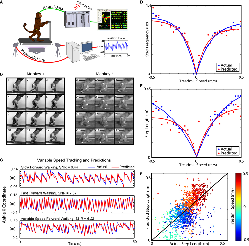
Figure 1. Experimental setup and Kinematic Analysis. (A) Diagram of the bipedal walking setup, consisting of a custom modified, hydraulically driven treadmill; wireless, 2-camera tracking of kinematics; and a MAP neural acquisition system (Plexon, Inc., TX, USA). (B) Video frames traced from typical step cycles from both monkeys. (C) Example tracking at multiple speeds. (D) The relationship between step frequency and walking speed. Blue points and curves represent the actual values, and red points and curves represent the extracted values. Each point in (D) and (E) represents an average over an epoch of constant treadmill speed during variable speed and direction sessions. (E) The relationship between step length and walking speed. As in (C), blue and red correspond to the actual and predicted values, respectively. (F) Actual step lengths versus extracted step lengths during all variable speed sessions. Blue dots represent backward walking while red/orange dots represent forward (see key on the right). Dots are clustered around the y = x line, indicating a match between the actual and predicted values.
Limb Movement Tracking
During experimental sessions, movements of the right legs of the monkeys were tracked using a wireless, video-based tracking system. The three dimensional coordinates of fluorescent markers applied to the hip, knee, and ankle were tracked using two cameras at a 30 Hz frame rate. Initially a commercial offline system (SIMI Motion 3D) was used for tracking purposes; in later sessions a custom real-time video-based tracking system developed in the lab was used (Peikon et al., 2007
). Data were cross-validated between the two systems to ensure that both produced equally accurate results and to ensure no biases were present in our custom system. To ensure consistent placement of the markers which were tracked on video, each of the monkeys was tattooed over the hip, knee, and ankle joints of their right legs. The markers themselves were applied before each session, and were made of fluorescent, non-toxic stage makeup. This approach offered several advantages. First, the markers were virtually weightless on the skin of the monkeys and thus did not impact the walking mechanics or cause distraction. Second, using fluorescent markers allowed us to achieve very high contrast ratios between markers and background on the recorded video stream. By turning visible light down to a low level, lowering the camera aperture, and bathing the experimental setup with a safe, filtered UV (or black) spotlight, the only significant source of visible light picked up by the cameras came from the markers which were being tracked. While the current tracking system is only capable of tracking the right leg, future versions will track both legs simultaneously, allowing us to investigate bipedal predictions. Figure 1
B illustrates frames of captured video that show an example of the bipedal walk cycle for each monkey. These figures have increased levels of ambient lighting to aid in viewing the step cycle. Both monkeys walked in a stereotyped bipedal manner and slightly leaned forward for comfort with arms holding a bar for support.
Kinematic Analysis
The monkeys’ limb tracking information was used to extract a number of experimentally relevant parameters in addition to the X, Y and Z coordinates of the joint markers. We extracted joint angles (hip and knee), foot contact with the treadmill, walking speed, step frequency and step length. All these parameters were calculated from the joint position data provided that the markers were not occluded. The episodes during which any of the markers was occluded (typically, when the monkeys turned their bodies) were excluded from the analyses. Our video analysis algorithm used a combination of mathematical techniques to calculate additional parameters. Treadmill speed was extracted from the video tracking data. The frequency of the step was extracted from the kinematic movement pattern of the ankle in the axis of treadmill motion. Furthermore, a combination of ankle displacement during the step phase and treadmill speed was used to extract stride length with respect to the moving surface of the treadmill. Foot contact was extracted first from a filtered height (Y-axis) threshold, which determined when the ankle joint was flat on the surface of the treadmill. However, a simple height threshold was not adequate to reject shuffling walking types, and a further check was instituted, which rejected periods without constant X-velocity of the ankle equal to treadmill speed.
Surgical and Electrophysiological Procedures
During the implantation surgeries, each of the two adult female rhesus macaques was anesthetized and placed in a stereotaxic apparatus (for a full description see Nicolelis et al. 2003
). All surgical procedures conformed to the National Research Council’s Guide for the Care and Use of Laboratory Animals (1996) and were approved by the Institutional Animal Care and Use Committee.
A series of small craniotomies were made, both to grant access to the brain for the microwire arrays and for anchoring the dental acrylic to the skull. In each animal, multiple microwire arrays were chronically implanted in several cortical areas (Figure 2
). The implanted areas were chosen based on previous cortical mapping studies (Nicolelis et al., 2003
; Tanji and Wise, 1981
; Wise and Tanji, 1981a,b
).
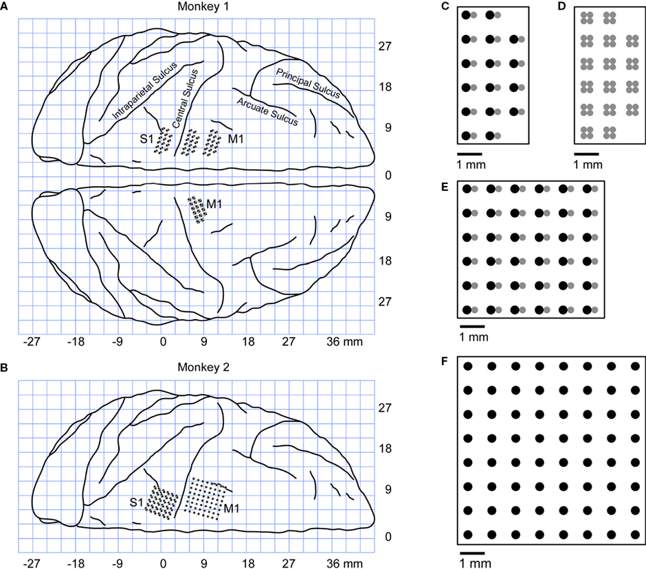
Figure 2. Diagram of cortical implants. A generic outline of cortical sulci (view from the top) is shown to illustrate the locations of the implants. Positive X coordinates correspond to rostral brain areas, while negative X coordinates correspond to caudal brain areas. (A) Implanted locations in Monkey 1. Both hemispheres were implanted. Two 32-electrode arrays were implanted in the left M1, one 32-electrode array in the left S1 and one 64-electrode array in the right M1. (B) Implanted locations in Monkey 2. The left hemisphere was implanted with two 64-electrode arrays, one placed in M1 and one in S1. (C–F) Configuration of the microelectrode arrays. The electrode shafts were arranged into 1-mm spaced grids. In multi-layered configurations, each shaft consisted of two (C,E) or four (D) microwires of different length. The difference in depth between the electrode layers was 0.3 mm.
Accordingly, multi-electrode arrays were inserted medially in the cortex approximately 2 mm in front of the central sulcus to target M1 and 2 mm behind it to target S1 (Figure 2
). The arrays were matched in size to the cortical representations of the hind limb. Monkey 1 was implanted with 50 μm tungsten chronic microwire arrays in the leg representation of both the primary somatosensory (S1) and primary motor (M1) cortices. One 8 by 8 square array with electrodes spaced 1 mm apart (inserted 2.5 mm deep in the cortex) was implanted rostral to the central sulcus. A 6 by 6 double-layered square array, using the same electrode spacing, was placed caudal to the central sulcus, 1.5 mm deep. In the double layer implant, the second layer of electrodes was 300–400 μm shallower than the first layer. Monkey 2 was also implanted with chronic microwire arrays in the leg representation of both the primary somatosensory (S1) and primary motor (M1) cortices. In M1, two 3 by 6 double layer arrays were implanted, while in S1 a single double layer 3 by 6 array was implanted. In all implants one layer was 300 μm deeper than the other layer. All electrodes in Monkey 2 were stainless steel microwires ranging in diameter from 40 to 60 μm. In both monkeys the placement of the electrodes was accomplished using stereotaxic coordinates and connectors for the arrays were embedded in a head cap made of dental acrylic.
Upon recovery from the surgical procedure, the receptive fields of individual S1 neurons and multi-unit activity were briefly examined in the awake monkeys by lightly touching and palpating their hind limbs. This examination confirmed that in both monkeys the implanted S1 sites represented the thigh, calf and the foot. No clear somatosensory responses were identified for the M1 implants. In Monkey 2, we briefly tested motor responses to cortical microstimulation under ketamine anesthesia. The microstimulation of M1 evoked hind limb movements due to proximal muscle contraction in agreement with Hatanaka et al. (2001) and Tanji and Wise (1981)
.
A total of 200–300 well sorted single units were recorded from implants in both monkeys per experimental session. After the monkeys were placed in the treadmill-mounted restraint, head stage amplifiers were attached to the head-cap connectors. A flexible wire harness, in turn, connected the headstages to a 128 channel Multichannel Acquisition Processor, or MAP, (Plexon, Inc., TX, USA) recording system. Neuronal units were sorted in real time using the templates defined in MAP software. The ratio of the amplitude of each sorted unit to the amplitude of electrical noise was, on average 3.34 ± 1.66 (mean ± standard error). The quality of online sorted single units was further examined by analyzing the refractory period, estimated from the interspike intervals. For each unit to be qualified as single unit, in addition to having a distinct shape and amplitude (Nicolelis et al., 2003
), it had to exhibit a refractory period greater than 1.6 ms (Hatsopoulos et al., 2004
). Using these criteria, 66.0% of the recorded units were single units, and 34.0% were classified as multi-unit neuronal activity. Overall, extraction of locomotion patterns from single units versus multi-units yielded similar results.
Electrophysiological recordings spanned 399 days in Monkey 1 and 56 days in Monkey 2. The implants were connected to a multichannel recording system (Plexon, Inc., TX, USA) using light flexible cables. The total number of simultaneously recorded units ranged from 180 to 238 in Monkey 1, depending on the recording day, and from 173 to 334 units in Monkey 2. In Monkey 1, we recorded from 111.2 ± 19.3 units (mean ± standard deviation; standard deviation reflects day to day variability) in left M1, from 38.1 ± 6.1 units in left S1 and from 55.6 ± 16.0 units in right M1. In Monkey 2, we recorded from 106.0 ± 19.9 units in left M1 and from 166.0 ± 31.0 units in left S1. Statistical analysis (Wilcoxon signed rank test) confirmed that average neuronal firing rates increased during walking in both M1 (P < 0.001) and S1 (P < 0.001) in each monkey. The average firing rate of M1 units was 7.5 ± 8.9 spikes/s during standing versus 15.0 ± 13.4 spikes/s during walking in Monkey 1, and 7.7 ± 8.7 spikes/s versus 11.4 ± 11.9 spikes/s in Monkey 2. In S1, the average rates were 8.7 ± 7.7 spikes/s during standing versus 16.6 ± 10.3 spikes/s during walking in Monkey 1, and 14.7 ± 12.9 spikes/s versus 24.3 ± 20.3 spikes/s in Monkey 2.
The MAP system was used for receptive field testing and for obtaining neuronal recordings during walking sessions. Electromyogram (EMG) signals were recorded from Monkey 1’s shaved skin surface, centered over the soleus, rectus femoris, and tibialis anterior muscles of both legs. Gold disc electrodes (Grass Instrument Co., RI, USA) were placed over conductive gel to obtain the EMG recordings. These EMGs were amplified up 10,000 times, band-pass filtered between 100 Hz and 1 kHz, rectified, and recorded using the MAP recording system to ensure consistent timing.
Models Utilized for Predicting Leg Kinematics
All the leg kinematic parameters extracted were reconstructed from neuronal ensemble activity using the linear decoding algorithm called the Wiener filter (Carmena et al., 2003
; Haykin, 2002
; Lebedev et al., 2005
; Wessberg et al., 2000
). The Wiener filter represented each decoded parameter as a weighted sum of neuronal rates measured before the time of decoding.

where X(t) is the value of the decoded parameter (for example, X-coordinate of the ankle marker) at time t, ni is the firing rate of neuron i, N is the total number of neurons, (j – 1)τ is tap delay for tap j, wij is the weight for neuron i and tap j, b is the y-intercept, and ε(t) is the residual error. For extracting marker coordinates, joint angles, and foot contact with the treadmill the tap length parameter τ was set to 50 ms, and the number of taps (time bins of neuronal data) was set to 10, that is neuronal rates were sampled in a 500 ms window preceding the time of decoding. For extracting slower modulated characteristics such as walking speed and step length, a 5 s sample window was used composed of ten 500 ms taps.
Prediction of leg kinematics was performed using multiple Wiener filters applied to the activity of the entire population of the recorded neurons or subpopulations recorded in separate cortical areas. Thus, the activity of simultaneously recorded cortical neural ensembles allowed us to simultaneously extract a variety of motor parameters: position of hip, knee, and ankle; hip and knee angles; as well as foot contact, direction of walking, and periods of standing still. We used multiple linear models (Wiener filters; Carmena et al., 2003
; Haykin, 2002
; Lebedev et al., 2005
; Wessberg et al., 2000
) to describe the relationship between these parameters and neuronal ensemble activity. To calculate model weights, first Eq. 1 was converted to matrix form as:

where X is the matrix of actual parameters, N is the matrix of neuronal rates, W is the weights of the model, ε is the error. Each row of N corresponds to a specific time and each column is a vector of data for a particular neuron and time lag. Since our models took into account ten lags, matrix N had ten columns for every neuron. The y-intercept was calculated from a column of ones prepended to matrix N. We then solved for matrix W by the following:

Each Wiener filter was first trained (i.e. the values of weights W were calculated) and then used as the decoder for new data. Accordingly, each experimental record (10–15 min) was split in two halves: the training data and the predicting data. The model was trained on the first half of the experimental data and predictions were obtained using the second half. Decoding was also conducted for the reverse arrangement: training the models on the second half and using it to predict the first half. In addition to these offline analyses conducted for 80 experimental records (66 with Monkey 1, 14 with Monkey 2), real-time extraction was performed in 22 experimental sessions with Monkey 1. For real-time extraction, the neuronal and kinematic data were first recorded for 5 min while multiple Wiener filters were trained, and then online extraction of walking parameters was performed for 5–10 min.
General and Switching Model
To test whether models trained to accurately predict motor parameters for a specific behavioral paradigm would retain general kinematic prediction accuracy during alternative behaviors (i.e. be able to generalize to new paradigms), we trained models for one direction of movement (e.g. forward walking) and tested them in the other (e.g. backward walking; for an example of this, see Figure 7
). This allowed us to ask whether a model that is trained to predict leg kinematics while the monkey walks forward would retain prediction accuracy when applied to sessions of backward walking and vice versa. Next, we investigated whether our models would benefit from training on a variety of behavioral data, in this case both forward and backward walking. To address these questions, a series of linear models were trained on selected behavioral epochs. The models were trained on: (1) only forward walking, (2) only backward walking, and (3) an equal mixture of the two walking paradigms. Each model was trained on an equal length of time to avoid any performance biases and then tested on its ability to accurately predict walking forward or walking backward separately.
The switching mode was used to handle the conditions in which the monkey’s locomotion consisted of two different paradigms: alternating periods of walking forward or walking backwards. Separate submodels were trained to decode each of these walking paradigms, and the paradigm predictor model served to detect the walking paradigm and select the appropriate submodel. The brief periods during treadmill mode switching when the monkey was standing still were classified as forward walking rather than introducing a third behavioral category. In our implementation, the switching model was a combination of three linear decoding models: a model for predicting forward walking, a model for predicting backwards walking and the paradigm predictor model (the switch). These models were arranged in a two layer structure (see Figure 7
F) with the paradigm predictor model controlling a toggle between the two kinematic submodels which were then shunted to the final output of the switching model. Thus, when it was determined that the monkey was walking forward, one submodel was used to produce the output, and when backwards walking was detected, the other submodel was used.
To avoid any bias in our comparisons between the generalized and switching model, they were both trained on the same amount of data. This means that while the single generalized model was trained over the full training window, each of the submodels of the switching model were only trained on the portions of the data when the monkey’s behavior fell in the relevant behavioral paradigm. Only the classifier portion of the switching model was trained on the full training window. This way, a true comparison of performance was achieved, and we could test whether the disadvantages of training the kinematic model on less total data were overcome by the advantages in prediction accuracy that come from behavioral segregation.
Model Performance Metrics
The signal to noise ratio (SNR) used in signal processing is a ratio between the power of the signal and the power of the noise, that is, the ratio of the squared amplitude of the signal and the squared amplitude of the noise. For our purposes, the signal was defined as the actual variable that we predicted. We calculated the variance, or power, of the signal by subtracting out the mean of the signal, then squaring and averaging the amplitude above or below that mean. The noise was the difference, or error, between the extracted and the actual signal. The error was calculated by subtracting the actual parameter from the extracted parameter, squaring the differences, then averaging to get the mean squared error, or the power of the noise. The ratio between these two was the SNR [or the signal to error ratio (SER)]. We then converted the ratio into a decibel (dB) scale:
Where X is the actual parameter, is the prediction of that parameter, Var is variance, and MSE is mean squared error. Theoretically, SNR can change from minus infinity (extremely poor predictions) to infinity (extremely good predictions). A SNR of 0 meant the signal and noise were in equal proportion in our predicted output. A SNR >0 meant we were extracting more signal than noise, and an SNR <0 meant there was more noise than signal, but the signal was still present for negative SNRs close to 0. SNRs equal to 10, 20, and 30 correspond to the ratio between the variances of 10, 100 and 1000, respectively
Additionally, Pearson’s correlation coefficient, R, between the known signal and the predicted output was calculated:
Where X is the actual parameter,  is the prediction of that parameter, cov is covariance, and σX and
  are the standard deviation of X and
  respectively. R can change in the range –1 to 1, with 1 corresponding to the highest possible correspondence between the actual and extracted values, and 0 corresponding to the absence of correspondence. Negative values of R, corresponding to an inverse relationship between the actual and extracted characteristics, occasionally occur when the extraction is poor, and R fluctuates around 0.
is the prediction of that parameter, cov is covariance, and σX and are the standard deviation of X and respectively. R can change in the range –1 to 1, with 1 corresponding to the highest possible correspondence between the actual and extracted values, and 0 corresponding to the absence of correspondence. Negative values of R, corresponding to an inverse relationship between the actual and extracted characteristics, occasionally occur when the extraction is poor, and R fluctuates around 0.Signal to noise ratio proved to be a more sensitive measure compared to R in these analyses. This was because R describes the correspondence of signal waveforms, but is insensitive to amplitude scaling and offsets. SNR is sensitive to errors introduced by these factors, which is important for the purposes of efficient BMIs that require that the output of the model matches the true signal in all aspects. Additionally, R often saturates quickly for large ensemble sizes, whereas SNR better tracks the dependency of model performance on the ensemble size. A metric similar to SNR, called SER was used in previous studies in which behavioral parameters were extracted from neuronal data (Kim et al., 2006
; Sanchez et al., 2002
).
Neuron Dropping Analysis
Neuron dropping analysis (NDA) is a conventional way to characterize the prediction performance of neuronal ensembles of different size (Carmena et al., 2003
; Lebedev et al., 2005
, 2008
; Wessberg et al., 2000
). In this analysis, a number of decoding models were trained on random subsets of sorted neurons, ranging in size from a single neuron to the entire bank of sorted neurons. To characterize the performance of these decoding models, we calculated neuron dropping curves which described decoding accuracy as a function of neuronal sample size (Wessberg et al., 2000
). The dropping curves were calculated by pooling randomly selected subsets of neurons and running the decoding model only for them. At each population subset size, five random subsets of neurons were generated and used to train separate predictive models. The predictive strength (SNR) of these models was calculated and plotted as scatter plots (for examples of this, see Figures 6A–F and 7D,F
). These scatter plots were then fitted using a power curve with simple linear decay:

where x is neuronal subset size and y is SNR. Five parameters were fitted to generate the curves: yoffset translated the entire curve up or down, xoffset translated left or right, yamplitude defined the height of the fitted curve, p was the power of the curve and described the rate of the climb in SNR with increases in neuronal subset size, and mdecay described the slope of the linear decay.
For our analysis examining predictions of several kinematic variables simultaneously from the same neuronal population, we used a modified version of the NDA. Random subpopulations of the neuronal ensemble were selected and used to train models for a random combination of kinematic parameters simultaneously. Simultaneous prediction accuracies were calculated to be the minimum SNR level reached by all the predicted variables at each neuronal ensemble size. The overall simultaneous prediction dropping curves were then fitted by power curves (Eq. 6). The curves were normalized and averaged across all combinations of kinematic variables. The final curves were thresholded at several levels of prediction accuracy (0.75, 0.85 and 0.95) to determine the minimum number of neurons needed to predict each number of kinematic variables simultaneously with the given level of accuracy (for an example of this, see Figures 8
A,B). Essentially, we calculated the expected number of neurons that would be required to predict, to a high accuracy threshold, any number of kinematic variables simultaneously in our experimental setup.
Real-Time System
We also developed a real-time BMI software suite capable of running all aspects of our experimental setups, including visual display, behavioral and multi-electrode neural recordings, model calculation and real-time predictions of kinematic and dynamic parameters. Written in Microsoft Visual C++, this BMI software suite can input behavioral data, multichannel extracellular single and multi-unit recordings, EMGs, and local field potentials.
Using a graphical user interface, models were trained to generate real-time predicted kinematics or EMGs from neural data. While our software suite currently implements the Wiener Filter, the Kalman Filter with optional principle components analysis dimensionality reduction, the n-th order Kalman Filter, and the n-th order Unscented Kalman Filter, in the real-time experiments described in this study we have used only the Wiener Filter option for extracting kinematic, dynamic, and EMG data.
The outputs of multiple real-time predictive models were displayed on a computer screen and simultaneously streamed over the network using a User Datagram Protocol.
Kinematics of Bipedal Walking
During walking, both monkeys adopted a posture in which they leaned slightly forward while holding a bar and episodically assumed a more upright posture (Figures 1
A,B). The right leg was video-tracked in real time using fluorescent markers applied to the hip, knee and ankle joints. The monkeys’ walking kinematics exhibited many basic features previously reported in both humans (Capaday, 2002
; Grieve and Gear, 1966
; Hirokawa, 1989
; Murray et al., 1964
, 1970
; Nielsen, 2003
; Perry, 1992
; Vaughan et al., 1992
) and monkeys (Hirasaki et al., 2004
; Matsuyama et al., 2004
; Mori et al., 2001
; Tachibana et al., 2003
). Step frequency rapidly increased as the treadmill speed increased from 0.05 to 0.2 m/s and began to plateau above 0.2 m/s (blue traces in Figure 1
D). Step frequency during backward walking plateaued at a slightly higher value (1.1 steps/s) versus forward walking (1.0 steps/s). Step length also increased as the treadmill speed increased with a slight tapering off at higher speed (blue traces in Figure 1
E). The stance phase constituted approximately 65% of leg stepping cycle (Monkey 1: 69.6 ± 13.1% during forward walking, 66.7 ± 16.2% during backward; Monkey 2: 57.6 ± 9.7% during forward).
During forward walking, the ankle and knee moved backward at a nearly constant speed after the foot touched the treadmill (Figure 3
A). At approximately mid-stance, the ankle started to lift, followed by the knee (Figure 3
B). These movements were accompanied by a lateral displacement (Z-dimension) of the ankle because of foot rotation (Figure 3
C). The knee angle monotonically increased during the stance phase as the knee joint extended during backward movement of the leg, and knee flexion started shortly before foot liftoff and continued during the swing (Figure 3
D). The soleus and rectus femoris were active during the stance phase and relaxed during the swing (Figure 3
E). The tibialis anterior was activated in a reciprocal manner: active during swing, relaxed during stance. This pattern of muscle activity is similar to EMG patterns during human walking (Capaday and Stein, 1986
; Ivanenko et al., 2008
; Kadaba et al., 1985
; Shiavi et al., 1987
; Winter and Yack, 1987
). Examples of video frame during stance and swing are shown in Figure 3
F
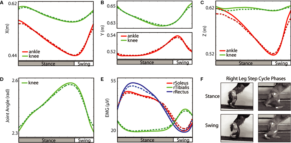
Figure 3. Average changes in walking parameters during the step cycle. The data from all experimental sessions during which the monkey walked in forward direction with EMGs recorded were averaged. The average portions of the stance and swing phases of the step cycle are shown below each plot. The hip movements are not illustrated because they were small. Solid lines show the actual values, and dashed lines show the values extracted from neuronal activity using the Wiener filter. Note the correspondence between the actual and extracted values. (A–C) X, Y, and Z position. (D) Knee angle. (E) EMG activity in the muscles of the right leg. (F) Examples of leg orientations classified as swing and stance.
The discharge rate for each of the cortical neurons peaked at a preferred phase of the step cycle (Figure 4
). The pattern of cortical activity during forward walking (Figure 4
A) was different for each recorded cortical area. In contralateral (left) M1, the number of neurons whose rates peaked during the stance was approximately equal to the number of neurons with the peak rate during the swing (61 ± 11 versus 63 ± 11, respectively, P > 0.05 Student’s t-test). However, since the swing was shorter than the stance, the density of peak rates per unit of the step cycle (the slope of the red line in Figure 4
A, 1st row) was lower for the stance phase (87.2 ± 18.6 peaks/s during stance versus 261.0 ± 29.0 peaks/s during swing, P < 0.001 Student’s t-test), especially for its initial phase preceding the stance to swing transition. Ipsilateral (right) M1, showed a different pattern of neural activity in this analysis which used the movements of the right leg to designate the step cycle, with more neurons peaking during the stance phase than the swing phase (38 ± 6 versus 20 ± 6, respectively, P < 0.001 Student’s t-test; Figure 4
A, second row), evidently because neural modulations there represented the out of phase movements of the left leg. Activity in S1 neurons was heavily concentrated at the swing phase, especially during the stance to swing transition (55.0% of S1 neurons had their peak activity in the 20% of the step cycle centered at the stance to swing transition; Figure 4
A, third row), when the foot was lifted from the treadmill surface.
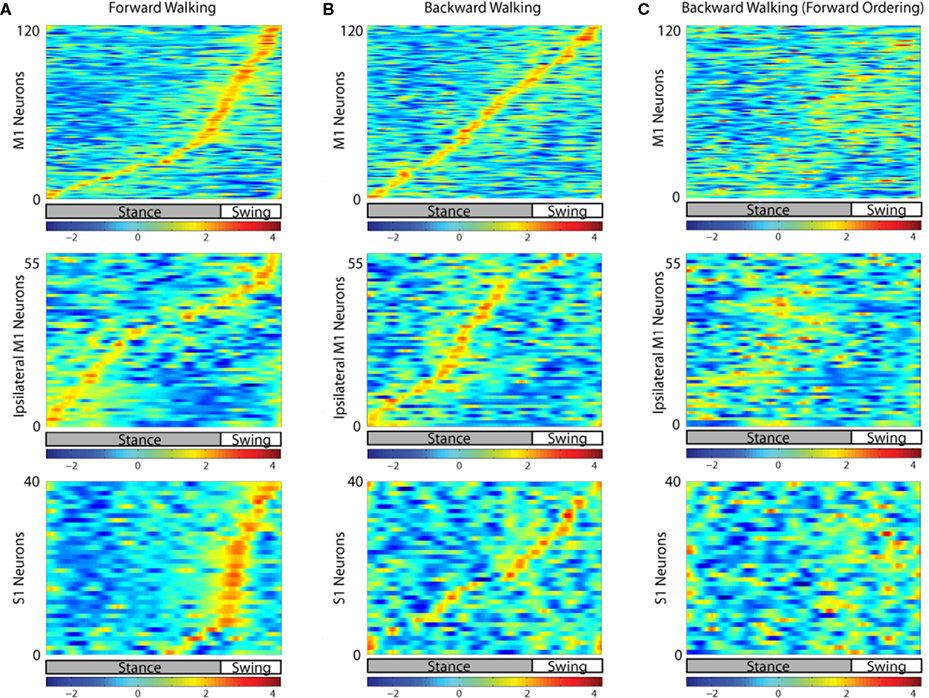
Figure 4. Neural activity in each cortical area during the step cycle. The neural data from experimental sessions during which the monkey walked in the forward and backward direction were separately averaged for many step cycles. Each horizontal line corresponds to the firing rate of a single neuron normalized by standard deviation (i.e. z-score). Each cortical area was analyzed separately (left M1 – top row, right M1 – middle row, left S1 – bottom row). The neurons were sorted by the phase of the step cycle during which they exhibited peak activity. The average durations of the stance and swing phases of the step cycle are shown below each plot. Swing was slightly longer during backwards walking. (A) Average neural activity during forward walking, ordered via peak activity during forward walking. (B) Average neural activity during backward walking, ordered via peak activity during backward walking. (C) Average neural activity during backward walking, ordered via peak activity during forward walking [i.e. neurons are ordered the same way in (A) and (C)].
A different pattern of ensemble modulations was revealed during backward walking (Figures 4
B,C). Notably, firing of the neurons tended to be more evenly spaced over the step cycle, especially in M1 (176.4 ± 29.4 peaks/s during stance versus 196.0 ± 19.6 peaks/s during swing, P > 0.05 Student’s t-test). When the cortical activity during backwards walking was sorted according to where the cells were most active in forward walking (compare Figures 4
A,C), it was apparent that there was little correspondence between individual cells’ activity peaks between forward and backward walking. However, there was still a slight tendency for the neurons that were active in the swing phase during forward walking to remain active during the swing during backward walking (44.4% of the neurons with peak rate during the swing) and the same tendency for the stance-phase neurons (80.1%). This tendency was statistically significantly greater (P < 0.005 Student’s t-test) than the percentage of neurons expected to stay in the same phase (29.9% and 70.1%) if there was no correlation between the neurons’ peak firing phases in forward versus backward walking. Thus, although leg kinematics were similar during forward and backward walking, the underlying neuronal patterns were substantially different.
Extracting Characteristics of Walking From Cortical Ensemble Activity
Multiple locomotion parameters were extracted using linear decoders which expressed the parameters as weighted sums of the neuronal firing rates (Carmena et al., 2003
; Haykin, 2002
; Lebedev et al., 2005
; Wessberg et al., 2000
). We decoded X (horizontal), Y (vertical), and Z (lateral) Cartesian coordinates of the leg joints, state of foot contact with the treadmill, step length and frequency, walking speed, and the EMGs of multiple leg muscles. Figures 4 and 5
E represent modulations of M1 and S1 discharges as “waves” of neuronal activity that occurred during each step. While the individual neuronal firing rates were highly variable from step to step at the millisecond scale (Figure 5
E), combining the activity of many neurons in 100 ms bins using the linear decoder produced accurate predictions of leg movements, as evident from average traces for joint coordinates (Figures 3
A–C), joint angle (Figure 3
D) and EMGs of leg muscles (Figure 3
E), as well as step frequency (Figure 1
D) and step length (Figures 1
E,F) derived from predictions of joint positions. Figures 5
A–E illustrates a 5 s epoch of forward walking during which 18 motor parameters were simultaneously extracted: joint coordinates (Figure 5
A), joint angles (Figure 5
B), state of foot contact (Figure 5
C) and EMGs (Figure 5
D). Figure 5
F depicts direct extraction of step length and walking speed (characteristics modulated at a slower pace) from a different 50 s epoch.
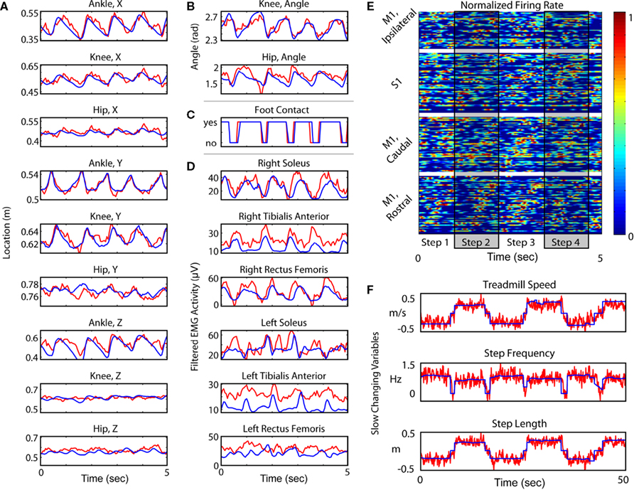
Figure 5. Extraction of multiple characteristics of walking. In all traces, blue shows actual and red shows extracted value. All variables are shown over the same 5 s window, except in (F), where slow changing variables are shown over a longer 50 s window. (A) Three dimensional position variables. The X axis is in the direction of motion of the treadmill; the Y axis is off the surface of the treadmill (axis of gravity); and the Z axis is lateral to the surface of the treadmill, but orthogonal to the direction of motion. (B) Joint angle variables. Hip angle is calculated assuming a fixed torso. (C) Foot contact, a binary variable defining the swing versus stance phase. (D) EMG variables. (E) Neuronal activity of 220 single units sorted via cortical area and by phase within the step cycle. Firing rate is normalized for every unit. (F) Slow changing state variables (walking speed, step frequency and step length) plotted over a 50 s time window.
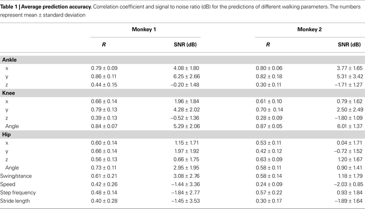
The average extraction performance is summarized in Table 1
. Overall, accuracy in predicting motor parameters was in line with that previously obtained for extracting arm movements from M1 activity (Carmena et al., 2003
; Lebedev et al., 2005
; Wessberg et al., 2000
). We observed SNR in the range –2 to 7 dB and correlation coefficients, R, in the range 0.2–0.9. In both monkeys, the best extracted parameters were those related to the X and Y coordinates of the ankle, and knee angle (SNR in the range 3.8–6.0 dB and R in the range 0.79–0.87). The Z coordinate (lateral movements) was not predicted as well, because of minimal lateral movements of the joints during walking sessions. Likewise, the small amount of hip movement produced during walking may have contributed to low prediction accuracy for the hip’s Cartesian coordinates compared to those of the knee and ankle. The X and Y coordinates of the knee and the hip were extracted with an average SNR in the range –0.7 to 4.3 dB and average R around 0.42–0.79. The average SNR and R for hip angle ranged from 0.9–3.0 and 0.58–0.73, respectively. Meanwhile, extraction accuracy for foot contact state (swing or stance) ranged from 1.2–3.1 in SNR and 0.58–0.61 in R, whereas the average SNR and R for the slowly modulated parameters were in the range –2.0 to 1.4 and 0.24–0.42 for walking speed, –1.8 to 0.9 and 0.48–0.57 for step frequency and –1.5 to 1.9 and 0.30–0.40 for step length. The low average accuracy of predicting the walking speed, especially in Monkey 2, reflected the fact that in many experiments the treadmill speed was constant for long periods of time and thus had very low variance. Predictions of EMGs (Figures 3E and 5D
) were better (P < 0.001, Student’s t-test) for the musculature of the right leg (SNR of 1.55 ± 0.39) than for the left leg (0.76 ± 0.17), likely because more neurons were recorded in the left hemisphere. Indeed, when prediction performance of equal size samples of neurons drawn from left versus right M1 was compared, contralateral M1 outperformed (P < 0.001, Student’s t-test) ipsilateral M1 in predicting either leg EMG.
Neuron Dropping Analysis
Figures 6
A–F depicts NDA for the extraction of walking parameters. Each dot in the scatter plots represents prediction accuracy (quantified as SNR) calculated for a randomly selected neuronal subset. The plots are fitted with exponential curves. NDA revealed that the prediction accuracy of joint coordinates monotonically increased with neuronal sample size (Figures 6
A–C). In the particular case of predicting foot contact, NDA revealed a pattern consistent with the known phenomenon of overfitting (Babyak, 2004
; Santucci et al., 2005
), i.e. the SNR increased as the sample grew to 50 neurons, and it decreased thereafter (Figure 6
D). In agreement with Table 1
, the Y-coordinates (vertical movements) for the ankle (Figure 6
A) and knee joints (Figure 6
B) were the most accurately predicted of all Cartesian coordinates. X was the second best extracted coordinate. Prediction accuracy for the knee and hip angles was comparable to the prediction of X and Y coordinates for these joints (Figures 6
B,C).
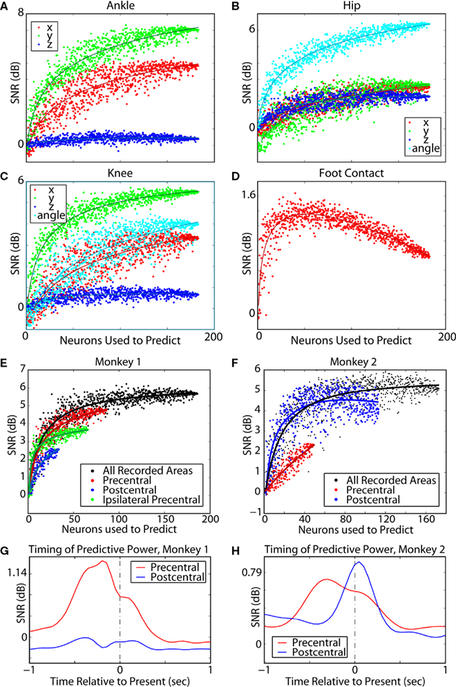
Figure 6. Neuronal dropping curves for simultaneously extracted variables. Dots represent SNR for the extraction of walking parameters using models trained on randomly selected neuronal populations of different sizes. In (A–C) red dots correspond to X coordinate, green dots to Y, and blue dots to Z. In (B,C) cyan dots correspond to joint angles for the respective joint. This analysis showed that prediction accuracy increased with the neuronal sample size [but see (D)]. Extraction analysis by cortical area was also performed for Monkey 1 (E,G) and Monkey 2 (F,H). In Monkey 1, more cells were recorded in M1 than in S1, whereas in Monkey 2 more cells were recorded in S1. (A) 3D coordinates of the ankle. (B) Joint angle and 3D coordinates of the knee. (C) Joint angle and 3D coordinates of the hip. (D) Foot contact, that is whether or not the monkey’s foot was on the ground. Foot contact was well predicted for smaller numbers of neurons but experienced overfitting for large numbers of neurons. (E,F) Neuronal dropping curves for the entire neuronal population and separate areas with extrapolated fits. (G,H) Prediction accuracy for M1 (red curves) and S1 (blue curves) as a function of time lag between the time of prediction and the time at which neuronal activity was sampled. In Monkeys 1 and 2, precentral neurons best predicted current kinematics using neuronal data in the past, indicating that neuronal modulations preceded motion. Monkey 2’s postcentral neurons had a peak in predictive power using future data, indicating that activity was a replica of the kinematics. In Monkey 1, the postcentral subpopulation did not have particularly strong predictive power in this analysis.
Neuron dropping analysis for predictions of the ankle X coordinate was also performed separately for different cortical areas (Figures 6
E,F). In both monkeys, walking parameters could be predicted using neuronal activity recorded in either M1 or S1 contralateral to the right leg, as well as ipsilateral M1 in Monkey 1, but none of these areas taken alone reached the prediction performance level of the entire population. Predictions using random populations drawn from each individual cortical area were statistically significantly worse than predictions from equivalently sized random populations drawn from all cortical areas (Student’s t-test, P < 0.001). For each area, the prediction performance improved with increases in population size. Slight overfitting was observed for S1 in Monkey 2 for ensemble sizes greater than 80 neurons (Figure 6
F, blue dots and curve). In Monkey 1, predictions from contralateral M1 neurons (Figure 6
E, red) were better than the predictions from ipsilateral M1 neurons (Figure 6
E, green) or contralateral S1 neurons (Figure 6
E, blue). In Monkey 2, predictions from S1 neurons were better than the predictions from M1 neurons (Figure 6
F).
The performance of the extraction algorithm, using M1 versus S1 neurons, was further examined using a timing analysis in which a single 50 ms time window was used to measure extraction accuracy at various lags with respect to the present time (time 0; Figures 6
G,H). Peaks in prediction accuracy for the lags preceding the present time (negative lags) indicated that neuronal modulations were predictive of future movements, suggesting a causal link between neuronal modulations and movements. Such a relationship was expected for M1 neurons and confirmed for both Monkey 1 (Figure 6
G) and Monkey 2 (Figure 6
H). Peaks for lags succeeding the present (positive lags) indicated a reverse relationship: present movements were the cause of future neuronal modulations. This was expected for S1 neurons, and confirmed in Monkey 2; the peak S1 extraction occurred at a positive lag (Figure 6
H). S1 activity was generally not strongly predictive at any lag in Monkey 1. There were minor peaks in S1 predictive power for both positive and negative lags (Figure 6
G). Still, the distinction between M1 and S1 was not clear cut because S1 modulations were capable of predicting motor parameters in the future (Figures 6
E–H).
Generalization Properties and a Switching Model
A linear decoder trained on a single walking paradigm (e.g. forward walking only or backward walking only) was able to accurately extract walking parameters during the same paradigm (SNR = 5.29 dB for the forward model applied to forward walking and SNR = 3.53 dB for the backward model applied to backward walking; Figures 7
A, left and 7B, right). However, predictive power was not retained when applied to predict a different paradigm (SNR = –2.91 dB for the forward model applied to backward walking and SNR = –2.77 dB for the backward model applied to forward walking; Figures 7
A,left panel and 7B,right panel). These results were confirmed by NDA (Figure 7
D).
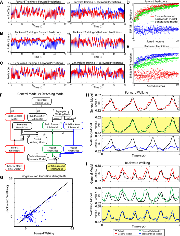
Figure 7. Generalized Training and the switching model. Panels A–C each represent a separate predictive model. In each, the left panel shows each model’s ability to predict the kinematics of walking during sessions where the monkeys walk forward while the right panel shows each model’s predictions of limb kinematics during periods of backward walking. The models accurately predicted conditions the same as the data they were trained upon but did not generalize well to conditions not contained within the training data set. The generalized model predicted either walking paradigm, but less accurately compared to paradigm-specific models. In response to these effects, a switching model (F–I) was designed that increased prediction accuracy for many kinematic parameters. (A) Actual and extracted traces of the X coordinate of the ankle for the forward walking model. Blue curves represent the actual position, and red curves represent the extracted position. (B) Traces for backward walking model. (C) Traces for generalized model. (D) Neuron dropping curves calculated by predicting forward walking using randomly selected neuronal populations with each model. (E) Neuron dropping curves calculated by predicting backward walking using randomly selected neuronal populations with each model. (F) Block diagram comparing the “switching” model with a generalized training model. Instead of using the same neuronal weights for all walking paradigms, the switching model uses two separate kinematic submodels running in parallel. Each model is optimized for a separate walking paradigm: forward and backward walking. A state predictive model determines walking mode and selects which of the two kinematic submodels becomes the final output. (G) Comparison of prediction strength of individual neurons during forward (abscissa) versus backwards (ordinate) walking. The prediction strength (R) was determined for single-neuron predictions of the X position of the ankle. While there is a general correlation between the Rs for these walking paradigms, there is a clear subpopulation of neurons with high Rs for forward, but not for backward walking. (H) Representative records of the X position of the ankle illustrating the predictive power of the switching model (the panel highlighted in yellow) versus generalized model (red curve) during forward walking. Note that the specialized model selected by the state predictive model (green curve) matches the original record (black curve) better than the generalized model (red curve) and the submodel for backward walking (blue curve). (I) Representative records for backward walking. The backward paradigm submodel selected by the state predictor (blue curve in the panel highlighted in yellow) matches the actual position (black curves) better than the generalized model (red curve) and the submodel for forward walking (green curve).
At the same time, general models trained on a mixture of both forward and backward walking (walking forward 45.1 ± 1.4% and backward 54.9 ± 1.4% of the time) accurately predicted both forward (Figure 7
C, left panel; SNR = 4.74 dB) and backward (Figure 7
C, right panel; SNR = 2.24 dB) walking separately, albeit slightly worse compared to the single paradigm models. This was also evident from NDA (Figure 7
D).
To recapture the lost prediction accuracy when using general models versus single paradigm models, we generated a multi-layer switching model (Figures 7
F–I). The switching model classified the subject’s walking as a number of sub-behaviors. That is, while the monkey was performing variable direction walking, walking was sub-classified into forward walking and backward walking periods. The switching model had two layers. The primary layer contained several independent submodels for kinematic variables, each one trained on data from a single sub-behavior. The secondary layer was a director layer that predicted the current behavioral mode (here, walking direction) for the subject and selected the appropriate kinematic submodel. The switching model outperformed the standard linear model trained during sessions with both forward and backward walking. The switching model improved the predictions of all kinematic variables on average by 13.8.
Predicting Multiple Parameters Simultaneously
Simultaneous extraction of many parameters essentially depended on the size of the neuronal population (Figures 8
A–C). Random subpopulations were pooled from the entire neuronal ensemble and used to predict several parameters simultaneously. For each parameter, prediction accuracy was normalized by its maximum value. The accuracy of simultaneous predictions was characterized by the normalized accuracy for the least well predicted parameter. Neuron dropping curves for this metric had less steep slopes when larger parameter sets were predicted (Figure 8
A). In other words, smaller neuronal populations could predict a few parameters simultaneously, and larger populations were required for predicting many parameters. This is illustrated in Figure 8
B, which shows that the number of neurons required to achieve a given minimum accuracy (75%, 85% or 95% of maximum prediction accuracy) increased with the number of simultaneously predicted parameters.
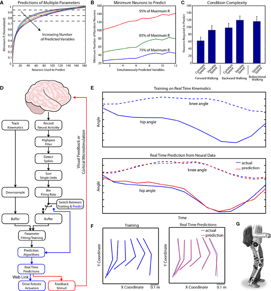
Figure 8. Simultaneous extraction of multiple parameters and real-time parameter extraction. (A) Neuronal dropping curves for extracting multiple parameters of walking. Each point on the curve represents the number of neurons needed to achieve a certain minimum level of prediction accuracy for each parameter (expressed as R normalized by the maximum value). The curves were fitted to the data for random groups of neurons used to predict random combinations of variables. This analysis revealed a slower rise for the multiple parameter dropping curves, indicating that larger neuronal populations were needed to predict multiple parameters simultaneously. (B) Number of neurons needed to attain a certain level of prediction accuracy (75%, 85% and 95% of maximum R) as the function of the number of simultaneously predicted variables. The curves were calculated from the neuron dropping curves shown in (A) These graphs show that the number of neurons needed for accurate prediction increased with the number of simultaneously extracted parameters of walking. (C) A comparison of the necessary number of neurons needed to accurately predict parameters in a variety of walking modes of different complexity. 95% of maximum R was set as the accuracy requirement. Bars show standard error. (D) Diagram outlining the operation of the real-time BMI. Real-time recordings of kinematic parameters and neural activity are filtered, binned and combined to train a series of Wiener models. Once the training is complete, the binned neural activity is sent into the models and kinematic output is generated. This kinematic output is used to drive robotic actuators. Feedback is sent back to the monkey using a visual display, or potentially, microstimulation pulses. (E) Training and prediction stages of the BMI. The panels show the average angles of hip and knee. In the top panel, training was occurring and there was not yet any predicted output. In the bottom panel extracted data was calculated (red), which matched actual kinematics (blue). (F) Training (left) and extraction (right) periods shown as the snapshots of leg configuration in treadmill surface centered coordinates. The configurations are projected onto the X–Y plane at 33 ms time steps to show a single step. Actual configurations of the leg are shown in blue, and predictions are shown in red. (G) Schematics of a future walking assist, exoskeletal BMI.
Similar to the result for the simultaneous extraction of multiple parameters, larger neuronal populations were required to predict complex patterns of walking compared to more simple walking patterns. For example, the number of neurons required to achieve 95% of maximum prediction accuracy for the X position of the ankle clearly increased when walking conditions of increasing complexity were employed (Figure 8
C). On average, 60 neurons were sufficient for predicting constant-speed walking in the forward direction. However, 90 neurons were needed to achieve this level of accuracy for variable-speed, forward walking. As complexity increased, more neurons were needed to maintain the same prediction accuracy. Thus, 95 neurons were required for predicting backward walking at constant speed, while 115 neurons were required for predicting backward walking at variable speed. Predicting variable-speed bidirectional walking required 110 neurons.
Real-Time Predictions of Leg Kinematics Using Cortical Neuronal Ensembles
Real-time prediction of kinematic variables (Figure 8
D) was performed in 22 daily recording sessions in Monkey 1. In each session, the first 5 min of walking were used for model training data. These data were sent to a buffer which was used to calculate a set of linear models for the leg kinematic parameters. These models were then used to generate real-time predictions from neural spike data alone. The actual and extracted joint angles are shown in Figure 8
E, and the actual and extracted leg configurations are shown in Figure 8
F. Real-time predictions were not statistically different from offline predictions (real-time SNR = 2.38 ± 1.14, offline SNR 2.46 ± 1.57, P > 0.05, Student’s t-test). The real-time system included a web link that could send the extracted kinematics to robotic appendages and return visual feedback (Figure 8
D). The operation of robotic devices under these conditions has been reported in abstract form (Cheng et al., 2007
; Lebedev et al., 2007
) and will be covered in detail in a future article.
In this study, we extracted bipedal walking patterns from the modulations of discharge rates of monkey S1 and M1 neuronal ensembles. While such modulations were expected from previous studies in quadrupeds (Armstrong and Marple-Horvat, 1996
; Beloozerova and Sirota, 1998
; Drew, 1993
; Prilutsky et al., 2005
; Widajewicz et al., 1994
), it was not clear until the present study whether cortical activity would be sufficient for accurate predictions of leg kinematics and EMGs during bipedal walking in primates. These findings have several implications. First, we have demonstrated the utility of using nonhuman primates for elucidating the neurophysiological mechanisms of bipedal locomotion. As such, we propose that chronic, multi-site cortical recordings could be used in the future to elucidate the neuronal mechanisms involved in upright posture control and bipedal walking. Second, as an implication for the BMI field, our findings provide the first proof of concept demonstration that, in the future, a neuroprosthetic for restoring bipedal walking in severely paralyzed patients can be implemented.
Cortical Neuronal Modulations During Bipedal Locomotion
Using cortical activity rather than subcortical locomotion centers for extracting walking patterns is not without controversy (Prochazka et al., 2000
). Although locomotion is conventionally recognized as a highly automated motor activity, subserved by spinal central pattern generators (Dietz, 2001
; Grillner, 2006
; Grillner et al., 2008
; Hamm et al., 1999
; Kiehn et al., 2008
; McCrea and Rybak, 2008
; Yamaguchi, 2004
), the involvement of the cerebral cortex in gait control has been reported in studies conducted in rodents (Hermer-Vazquez et al., 2004
), cats (Armstrong and Marple-Horvat, 1996
; Beloozerova and Sirota, 1993
), and monkeys (Courtine et al., 2005b
). Moreover, cortical involvement in locomotion seems to increase during more demanding tasks, especially those that require visual feedback (Armstrong and Marple-Horvat, 1996
; Beloozerova and Sirota, 1993
; Drew et al., 2008
).
Sampling from large populations of M1 and S1 neurons allowed us to analyze activity modulations in hundreds of simultaneously recorded neurons. Both M1 and S1 neurons modulated their firing rate in relationship to the stepping cycle. Firing for each neuron peaked at a particular phase of the stepping cycle. Given the large number of neurons that we recorded, it was unrealistic to examine in detail the properties of each neuron in order to determine which motor or sensory responses determined its step cycle modulations. Therefore, we used a population based approach in which cycle modulations of individual neurons each contributed to the extraction of the step cycle at every time step, and more precise extractions were obtained by combining the information from many neurons. We also showed the benefits of utilizing multi-site recordings to predict locomotion kinematic parameters. This approach was beneficial because neuronal modulations from different cortical areas provided the diversity and richness of cortical signals needed for the accurate extraction of motor parameters under different behavioral conditions. In this context, we consistently observed superior performance of neuronal populations drawn from several cortical areas compared to the performance of populations drawn from a single area.
Extracting of Multiple Parameters of Bipedal Walking
Walking patterns were extracted using multiple linear models. As in previous studies in which predictions of arm movements were obtained, NDA showed that large neuronal ensembles were needed for accurate predictions of leg kinematic parameters. Thus, larger neuronal samples were required for simultaneous extraction of multiple walking parameters. Small populations of relatively specialized neurons could accurately extract only a subset of locomotion parameters, and additional neurons were required to improve the extraction of the other parameters. As a corollary to this finding, larger neuronal populations were required as task complexity increased. These results support our previous suggestion that, to efficiently control a multiple degree of freedom neuroprosthetic, recording the activity of large ensembles of cortical neurons will be necessary (Carmena et al., 2003
; Lebedev et al., 2007
; Wessberg et al., 2000
).
M1 Versus S1 Contributions to the Prediction of Leg Kinematics
Both M1 and S1 neurons contributed significantly to the predictions of leg kinematics. As expected, M1 modulations were more informative for predicting future values in the parameters of walking, whereas S1 modulations better predicted the past values of the parameters. However, this distinction was not absolute, particularly in Monkey 2 in which accurate predictions of future values of locomotion parameters could be obtained from S1 activity. While repetitive nature of the movement may be one contributor to S1 predictive power, predictions obtained from S1 activity could also reflect centrally generated signals related to communication between motor and sensory areas and efferent copies (Chapin and Woodward, 1982
; Fanselow and Nicolelis, 1999
; Lebedev et al., 1994
).
Generalized Training
The computational models of a BMI take advantage of correlations between neuronal firing modulations and behavioral parameters to generate their predictions. These correlations do not necessarily reflect a direct relationship or causation between neuronal discharges and the predicted parameters (Lebedev and Nicolelis, 2006
). Consequently, a model trained under one set of conditions may not perform well when the conditions are changed and the correlation between the neuronal discharges and behavioral parameters are altered. We observed this effect when we attempted to predict different locomotion patterns (Figure 7
). Models trained on forward walking did not accurately predict backward walking and vice versa. This drop in prediction performance occurred because of the differences in neuronal modulations during the step cycles of forward walking versus backwards walking (Figure 4
). Such an effect was expected because leg dynamics change dramatically during backwards walking despite relatively small changes in leg kinematics (Thorstensson, 1986
). It was only when the models were trained on a wider variety of patterns that they improved their ability to predict more diverse behaviors. Given that motor cortical neurons may represent muscle activity, limb kinematics and their combinations (Kakei et al., 1999
), which all change in complex ways when behavioral paradigms are altered, this result is not entirely surprising. For instance, the pattern of muscle activation may become different for a given leg orientation in a new walking condition, and muscle-representing neurons would introduce errors in predicted kinematics. It is only when the linear models are trained on several behaviors that the kinematics can be accurately extracted. These results suggest that in order to build a neuroprosthetic that is both accurate and versatile in restoring locomotion patterns, it will be necessary to generate a training protocol which is varied enough so that the employed models learn to predict a large set of behaviors.
Switching Model
While generalized training had the advantage of producing models that provided accurate predictions of the various behavioral paradigms included in the training data set, generalized models predicted with less accuracy than specific models designed for a single walking paradigm. To recapture some of this lost accuracy, we developed a switching model that selected the appropriate specific model once a switch in the walking paradigm was detected. Algorithms based on the idea of switching state spaces have been previously proposed for extracting arm movements from neuronal modulations (Kim et al., 2003
; Wu et al., 2004
). While the switching model has many advantages and it increased the accuracy of predictions throughout this experiment, it does carry some potential drawbacks. For variables that do not behave differently between behavioral paradigms, there is little lost accuracy to recapture, and segregating the data in the training set into smaller sections for each submodel can have a detrimental effect, that is, the lower quantity of training data can produce a less accurate model. Additionally, the performance of the switching model is heavily dependent on the performance of the state predicting model that chooses which kinematic submodel is selected
Real-Time Bmi for Reproduction of Locomotion Patterns
Since one of the long-term goals of this research is to build a neuroprosthetic device for the restoration of locomotion in paralyzed subjects, we tested the performance of our decoding algorithm using a real-time BMI suite that incorporated MAP recording hardware (Plexon Inc., TX, USA), a custom wireless video tracking system and a set of real-time prediction algorithms. The BMI suite sampled the activity of up to 512 neuronal units and converted this neuronal activity into the predictions of multiple degree of freedom kinematic and behavioral parameters. The BMI suite streamed the predictions using an internet protocol. The successful implementation of this apparatus allowed us to obtain a proof of concept that a real-time BMI for the reproduction of locomotion can be implemented in the future as the core of a neuroprosthetic device aimed at restoring bipedal locomotion in severely paralyzed patients.
Restoration of Locomotion Behaviors Using a BMI
Based on these results, we propose an approach to restore locomotion in patients with lower limb paralysis that relies on using cortical activity to generate locomotor patterns in an artificial actuator, such as a wearable exoskeleton (Figure 8
G; Fleischer et al., 2006
; Hesse et al., 2003
; Veneman et al., 2007
). This approach may be applicable to clinical cases in which the locomotion centers of the brain are intact, but cannot communicate with the spinal cord circuitry due to spinal cord injury. The feasibility of employing a cortically driven BMI for the restoration of gait is supported by fMRI studies in which cortical activation was detected when subjects imagined themselves walking (Bakker et al., 2007
, 2008
; Iseki et al., 2008
; Jahn et al., 2004
) and when paraplegic patients imagined foot and leg movements (Alkadhi et al., 2005
; Cramer et al., 2005
; Hotz-Boendermaker et al., 2008
). Event-related potentials also demonstrated cortical activations in similar circumstances (Halder et al., 2006
; Lacourse et al., 1999
; Muller-Putz et al., 2007
). Further support for this idea comes from recent studies of EEG-based brain-computer interfaces for navigation in a virtual environment in healthy subjects (Pfurtscheller et al., 2006
) and paraplegics (Enzinger et al., 2008
).
While a cortical BMI based neuroprosthesis that derived all its control signals from the user would have to cope with the lack of signals normally derived from subcortical centers, such as the cerebellum, basal ganglia and brainstem (Grillner, 2006
; Grillner et al., 2008
; Hultborn and Nielsen, 2007
; Kagan and Shik, 2004
; Matsuyama et al., 2004
; Mori et al., 2000
; Takakusaki, 2008
), these problems may be avoided by an approach which only derives higher level leg movement signals from brain activity, while allowing robotic systems to produce a safer, optimum output. The challenge of efficient low-level control could be overcome by implementing “shared brain–machine” control (Kim et al., 2006
), i.e. a control strategy that allows robotic controllers to efficiently supervise low-level details of motor execution, while brain derived signals are utilized to derive higher-order voluntary motor commands (step initiation, step length, leg orientation).
A cortically driven BMI for the restoration of walking may become an integral part of other rehabilitation strategies employed to improve the quality of life of patients. In particular, it may supplement the strategy based on harnessing the remaining functionality and plasticity of spinal cord circuits isolated from the brain (Behrman et al., 2006
; Dobkin et al., 1995
; Grasso et al., 2004
; Harkema, 2001
; Lunenburger et al., 2006
). Indeed, cortically driven exoskeletons may facilitate spinal cord plasticity, helping to recover locomotion automatisms. Additionally, cortically driven neuroprostheses may work in cohort with rehabilitation methods based on functional electrical stimulation (FES; Hamid and Hayek, 2008
; Nightingale et al., 2007
; Wieler et al., 1999
; Zhang and Zhu, 2007
). In such an implementation, the BMI output could be connected to a FES system that stimulates the subject’s leg muscles. Finally, there is the intriguing possibility of connecting the BMI to an electrical stimulator implanted in the spinal cord, a strategy that may help induce plastic reorganization within these circuits.
Altogether, our results indicate that direct linkages between the human brain and artificial devices may be utilized to define a series of neuroprosthetic devices for restoring the ability to walk in people suffering from paralysis.
The authors declare that the research was conducted in the absence of any commercial or financial relationships that could be construed as a potential conflict of interest.
This work was supported by the Anne W. Deane Endowed Chair Fund and by Telemedicine and Advanced Technology Research Center (TATRC) W81XWH-08-2-0119 to MALN. We are grateful to Gary Lehew for building the experimental treadmill, Timothy Hanson, Zheng Li and Joseph O’Doherty for programming the BMI software, Dragan Dimitrov, Laura Oliveira and Aaron Sandler for conducting the implantation surgery, Weiying Drake, Tamara Phillips, Benjamin Grant and Jenna Maloka for experimental support, and Susan Halkiotis for help with manuscript preparation.
Enzinger, C., Ropele, S., Fazekas, F., Loitfelder, M., Gorani, F., Seifert, T., Reiter, G., Neuper, C., Pfurtscheller, G., and Muller-Putz, G. (2008). Brain motor system function in a patient with complete spinal cord injury following extensive brain-computer interface training. Exp. Brain Res. 190, 215–223.
Sanchez, J. C., Kim, S. P., Erdogmus, D., Rao, Y. N., Principe, J. C., Wessberg, J., and Nicolelis, M. A. (2002). Input-output mapping performance of linear and nonlinear models for estimating hand trajectories from cortical neuronal firing patterns. In: Proceedings of the 2002 12th IEEE Workshop on Neural Networks for Signal Processing, Valais, Switzerland, pp. 139–148.
Wood-Dauphinee, S., Exner, G., Bostanci, B., Exner, G., Glass, C., Jochheim, K. A., Kluger, P., Koller, M., Krishnan, K. R., Post, M. W., Ragnarsson, K. T., Rommel, T., and Zitnay, G. (2002). Quality of life in patients with spinal cord injury – basic issues, assessment, and recommendations. Restor. Neurol. Neurosci. 20, 135–149.