Recurrent network for multisensory integration-identification of common sources of audiovisual stimuli

We perceive our surrounding environment by using different sense organs. However, it is not clear how the brain estimates information from our surroundings from the multisensory stimuli it receives. While Bayesian inference provides a normative account of the computational principle at work in the brain, it does not provide information on how the nervous system actually implements the computation. To provide an insight into how the neural dynamics are related to multisensory integration, we constructed a recurrent network model that can implement computations related to multisensory integration. Our model not only extracts information from noisy neural activity patterns, it also estimates a causal structure; i.e., it can infer whether the different stimuli came from the same source or different sources. We show that our model can reproduce the results of psychophysical experiments on spatial unity and localization bias which indicate that a shift occurs in the perceived position of a stimulus through the effect of another simultaneous stimulus. The experimental data have been reproduced in previous studies using Bayesian models. By comparing the Bayesian model and our neural network model, we investigated how the Bayesian prior is represented in neural circuits.

1. Introduction

We are surrounded by many sources of sensory stimulation, i.e., many sights and sounds. Moreover, we can recognize who is speaking in a conversation even when there are many people and sounds around us. To perform such recognition, we have to integrate correct pairs of stimuli; the movements of a person's mouth and the sound of his/her voice. Thus, it is important to determine how we judge which pairs of audiovisual stimuli are related and how we integrate related cues. That is, we must study multisensory integration in order to elucidate how our brains link multiple sources of information. There is a good example of audiovisual integration known as the ventriloquism effect in which the perceived location of a ventriloquist's voice is altered through the movement of a dummy's mouth (Howard and Templeton, 1966). It is also known that the ventriloquism effect can be elicited under artificial experimental conditions such as a spot of light or a beep (Bertelson and Aschersleben, 1998; Pavani et al., 2000; Lewald et al., 2001; Hairston et al., 2003; Alais and Burr, 2004; Wallace et al., 2004). Several theoretical models based on Bayesian inference have been proposed to explain the data from psychophysical experiments on the ventriloquism effect (Körding et al., 2007; Sato et al., 2007). Although Bayesian inference gives a normative account as to the computational principle, it does not indicate how the nervous systems actually implement the computation.

To provide insights into the neuron dynamics related to sensory integration, several studies have constructed neural network models that implement Bayesian inference (Pouget et al., 1998; Ma et al., 2006). When stimuli have a common cause, their models are able to extract encoded information from the activities of large populations of neurons as reliably as the maximum likelihood is able to do (Deneve et al., 1999; Latham et al., 2003). However, when stimuli have distinct sources, the models cannot work correctly because they bind cues even when the stimuli do not have the same source. When the stimuli have distinct causes, the brain has to estimate the causal structure of the stimuli and extract information separately from each stimuli. We constructed a recurrent network model that can implement computations related to multisensory integration by changing the method of divisive normalization in the model of Deneve et al. (1999). We found that our model could estimate not only the locations of the sources of the stimuli but also the number of sources. By using computer simulation, we showed that the model accounts for the data of psychophysical experiments that have been explained by the Bayesian model. To elucidate how our brains implement a Bayesian prior distribution, we tried to determine which neural connectivities represent the prior distribution.

2. Model

We constructed a single layer recurrent network consisting of N = 1000 analog neurons with identical spatial receptive fields. Here, we will label a neuron, i, by an angle θ_i and express the firing rate as a function of θ; therefore, a neural state, u_i, describes the firing rate of the neuron population (including both excitatory and inhibitory neurons) with the preferred angle, i. In order to reduce the number of parameters and facilitate analysis of the system's behavior, we will study a simpler model, in which the excitatory and inhibitory populations are collapsed into a single equivalent population. To model a cortical hypercolumn consisting of a single layer of neurons, we assumed that the preferred orientations are evenly distributed from −50 to 50 deg and divided 100 deg into N = 1000 sections, that is, θ_i = 0.1 × i − 50 deg. The neural state, u_i, is determined by inputs, a_i, as

$\begin{array}{cc}{a}_i(t)=h_i+{\displaystyle \sum _j^N{J}_{ij}}{u}_j(t),& (1)\end{array}$

where h_i represents an external input and the second term of the right-hand side of the equation represents a recurrent input. Using a_i, we defined the firing rate u_i as

$\begin{array}{cc}{u}_i(t+1)=\frac{{[a_i(t)]}_{+}}{1+\frac{1}{N}{\displaystyle {\sum }_j^N{[a_j(t)]}_{+}}}.& (2)\end{array}$

To keep u_i positive, we used the threshold linear function [a_i]₊ ([a_i]₊ = a_i if a_i > 0, [a_i]₊ = 0 if a_i ≤ 0). To control the gain of the firing rate u_i, we used divisive normalization Carandini et al. (1997). The interaction in the network turns noisy input into a smooth hill shape. The cap coordinate of the hill gives an estimate of the orientation. In a previous study, Deneve et al. (1999) defined a function u_i(t) in terms of the square of the input a_i

$\begin{array}{cc}\widehat{u}(t)=\frac{a_i{(t)}^2}{1+\frac{1}{N}{\displaystyle {\sum }_j^N{a}_j}{(t)}^2}.& (3)\end{array}$

In order to collapse the excitatory and the inhibitory populations into a single equivalent population, we assumed that the synaptic weight, J_ij, is a Mexican-hat-type connectivity: excitations are given to nearby neurons, inhibitions to distant neurons (Figure 1; Amari, 1977; Shadlen et al., 1996). We defined:

$\begin{array}{cc}{J}_{ij}=\frac{M_1}{\sqrt{2\pi {\sigma }_1^2}}\exp \left(\frac{-{({\theta }_i-{\theta }_j)}^2}{2{\sigma }_1^2}\right)-\frac{M_2}{\sqrt{2\pi {\sigma }_2^2}}\exp \left(\frac{-{({\theta }_i-{\theta }_j)}^2}{2{\sigma }_2^2}\right).& (4)\end{array}$

The parameters σ₁, σ₂, respectively define the range of the excitatory connection and lateral inhibition. Here, we set M₁ = 28, M₂ = 10, σ₁ = 1.5 [deg], and σ₂ = 3 [deg]. The two features in our model, i.e., weak normalization and lateral inhibition, make differences between ours and Deneve's model, and they enable our model to reproduce the results of psychophysical experiments (as discussed in the Results).

FIGURE 1

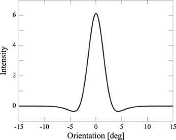
Figure 1. Mexican-hat-type connectivity J_ij: excitations are given to nearby neurons, inhibitions to distant neurons.

Let us consider an external input, h, from either a preceding layer or from the external world. The external input of neuron i, h_i, is dependent on the orientation encoded in the previous layer and is Gaussian distributed with mean 〈h_i〉 and variance σ²_i. We define

$\begin{array}{cc}{h}_i\text{}=\text{}\frac{M_V}{\sqrt{2\pi {\sigma }_V^2}}\exp \left(-\frac{\text{}{({\theta }_i-x_V)}^2}{2{\sigma }_V^2}\right)\text{}+\frac{M_A}{\sqrt{2\pi {\sigma }_A^2}}\exp \text{}\left(-\frac{{({\theta }_i-x_A)}^2}{2{\sigma }_A^2}\right)\text{}+\text{}{z}_i,\text{}& (5)\end{array}$

where z_i denotes noise. We set σ²_i to the mean activity, i.e., σ²_i = 〈h_i〉, which better approximates the noise measured in the cortex Shadlen and Newsome (1994). The standard deviations σ_V and σ_A respectively represent the uncertainties of the visual and audio input. Note that the strength of the input activity, $\frac{M}{\sqrt{2\pi {\sigma }^2}}$, is determined not only by M but also by the uncertainty of the input, σ, in our model. We assumed that the visual input is more reliable than the audio input. To investigate the effect of the difference in uncertainty between visual and audio input, we fixed M_V = M_A = 10, σ_V = 1 [deg], and σ_A = 2 [deg]. Thus, the input strength of visual input is larger than that of audio input, i.e., $\frac{M_V}{\sqrt{2\pi {\sigma }_V^2}}>\frac{M_A}{\sqrt{2\pi {\sigma }_A^2}}$. An example of external input to the network is given in Figure 2.

FIGURE 2

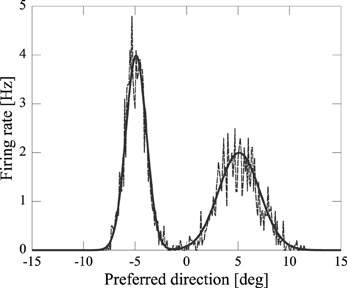
Figure 2. Example of input to the network (broken line) and mean input (solid line).

Now let us explain x_V and x_A in Equation 5. x_V and x_A represent the input locations of audiovisual stimuli. We assume that the audio and visual stimuli are Gaussian distributed:

We fix σ_Vx = 3 [deg] and σ_Ax = 6.5 [deg]. Here, (μ, σ_p) means a Gaussian distribution with mean μ and standard deviation σ. The external input, h_i, is given in the initial five steps (0 ≤ t ≤ 4). The noisy input, h_i, determines the initial state of u_i [a_i(0) = h_i]. Because of the recurrent connections and neural dynamics (See Equation 1 and Equation 2), the noisy neural states become a smooth hill whose peak indicates the estimated position of the audiovisual stimuli (Figure 3).

FIGURE 3

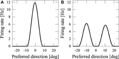
Figure 3. Output of network model. (A) Common cause; (B) independent cause.

3. Results

By using computer simulations, we showed that our network model can estimate the position(s) of the sources of audiovisual stimuli with a disparity between the stimuli. We found that while previous models could not reproduce psychophysical experiments of the audiovisual integration, our results are consistent with both experimental observations and Bayesian inference. If the disparity of the input stimuli was small (x_A − x_V = 5 [deg]), the stimuli were integrated with a high rate (about 70%) (Figure 3A). If the disparity was large, they were estimated as distinct stimuli (Figure 3B), something which could not be reproduced in previous models where the normalization term in Equation 2 is determined by the square sum Deneve et al. (1999). We found that in the previous network model, they were estimated not as distinct stimuli but as a united stimulus for any spatial disparity. The failure of Deneve's model to reproduce the phenomenon is partly the result of the strong divisive normalization they used (Equation 2), because the strong divisive normalization prunes weak multiple input peaks and extracts the maximum peak. Another reason for the failure of reproduction is the lateral inhibition between neurons. Figure 4 compares the models in the case of independent causes. Similarly to the Deneve's model, in a weak normalization model without lateral inhibition, they were estimated not as distinct stimuli but as a united stimulus for any spatial disparity, as shown in Figure 4B Marti et al. (2013). Thus, both weak normalization and lateral inhibition in our model are important for reproducing the results of the psychophysical experiments on audiovisual integration.

FIGURE 4

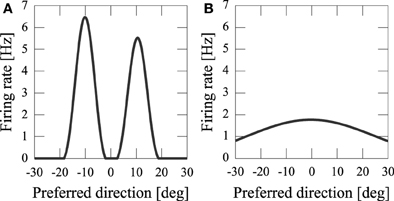
Figure 4. Model comparison in the case of independent cause. (A) Our network model; (B) weak normalization model without lateral inhibition.

3.1. Effect of Sensory Noise

We assumed that information about the orientations of the audiovisual stimuli from sense organs, x_V, x_A, are corrupted with sensory noise. This noise makes the output probabilistic (Figure 5A). If we didn't add noise, the number of sources would be completely determined by the spatial disparity D (Figure 5B). Experiments have shown that people estimate the number of sources stochastically Wallace et al. (2004).

FIGURE 5

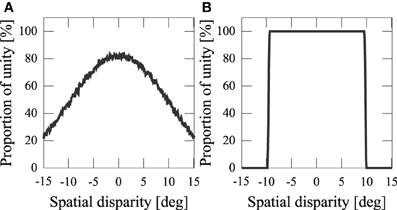
Figure 5. Frequency of the network model estimating stimuli having a common cause. (A) Proportion of unity with sensory noise [x_V ~ (S_V, σ²_Vx), x_A ~ (S_A, σ²_Ax)]. (B) Proportion of unity without noise (S_V = x_V, S_A = x_A).

3.2. Bias

Psychophysical experimental research has reported that when audiovisual stimuli were estimated as distinct stimuli, the estimated position of the auditory stimuli was away from the actual position of the auditory input Wallace et al. (2004). To examine how the perception of common versus distinct causes affects the estimation of the auditory stimuli position, Ŝ_A, we calculated the localization bias,

$\begin{array}{cc}bias=\frac{{\widehat{S}}_A-S_A}{S_V-S_A}.& (7)\end{array}$

We performed 500 simulations and averaged the localization bias for each disparity between the audiovisual stimuli and for each case, i.e., common and distinct. We compared our model and the previous model of Deneve et al. (1999). In the previous model, the stimuli were unified with any spatial disparity (Figure 6A). The value of the localization bias was nearly 100% with all spatial disparities. This means their model estimated the audio stimulus as noise. Our model made estimates about whether stimuli have a common cause or distinct causes stochastically (Figure 6B). When two stimuli were unified, the localization bias was nearly 80%. This indicates that when there was a common cause, the estimated auditory stimulus would be at a position that was on average very close to that of the visual stimulus. On the other hand, in the case of distinct causes, the localization bias took a negative value and was increasingly negative for smaller disparities. These results indicate that the estimated auditory position seems to be pushed away from the location of the visual stimulus, as was experimentally observed Wallace et al. (2004).

FIGURE 6

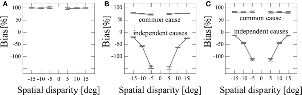
Figure 6. Localization bias with spatial disparity D. Error bars represent SEMs. (A) Previous model Deneve et al. (1999). (B) Proposed model. (C) Bayesian model Körding et al. (2007); Sato et al. (2007). “Common cause” refers to the situation in which the model regarded that two sensory signals have a common cause (i.e., the network converged to a single bump state) and “independent cause” refers to the situation in which the network regarded that two sensory signals have independent causes (i.e., the network converged to a state of two single bumps or the MAP estimate of the Bayesian model corresponds to two sources). The negative bias indicates that the perceived auditory position is on the opposite side of the true position with respect to the position of the visual stimulus.

4. Bayesian Prior in a Neural Network

Bayesian inference is a method of reasoning that combines prior knowledge about the world with current input data. To be more precise, from experience we may learn how likely two co-occurring signals (visual and auditory signals) are to have a common cause versus two independent causes. Using the Bayesian prior, a Bayesian inference model integrates those pieces of information to estimate if there is a common cause and to estimate the positions of cues. Previous studies have reported that Bayesian inference could explain the pattern of localization bias as reproduced by our model (Figure 6C) (Körding et al., 2007; Sato et al., 2007). Considering that our neural network model and the Bayesian model could explain the same psychophysical experiment, there should be a neural connection in our model that represents prior information. We searched for the parameter of our network model that corresponded to the prior information of the likelihood of sensory integration.

4.1. Multisensory Integration in the Neural Network

To simplify the comparison between the network model and Bayes model, let us consider a case in which we receive sensory inputs without noise (x_V = S_V, x_A = S_A). The distance between audiovisual stimuli D determines the causal structure in this case (Figure 5B), and we can determine the integration threshold D^Net₀ (the distance within which the auditory and visual signals are integrated). When D^Net₀ is determined, we can calculate the proportion of integration with noise as follows. When the distance between the audiovisual inputs, x_V − x_A = D_input, is lower than D^Net₀, stimuli integrate. D_input is drawn from a normal distribution with mean S_V − S_A = D, which is the distance between the original positions of the audiovisual stimuli, and standard deviation $\sqrt{{\sigma }_{Vx}^2+{\sigma }_{Ax}^2}$, which is the sum of the auditory and visual noise. Using D^Net, we obtain the proportion of integration as a function of D,

$I(D)={\displaystyle {\int }_{D-D_0^{Net}}^{D+D_0^{Net}}\frac{1}{\sqrt{2\pi ({\sigma }_{Vx}^2+{\sigma }_{Ax}^2)}}}\exp \left(-\frac{t^2}{2({\sigma }_{Vx}^2+{\sigma }_{Ax}^2)}\right)dt.$

D^Net₀ determines the likelihood of sensory integration. We investigated the relationship between the parameters of the neural connection J_ij and the Bayesian prior distribution regarding the integration threshold.

4.2. Integration Threshold in Bayesian Model

Using the Bayesian approach, we can also calculate the integration threshold D^Bay₀ (distance within which auditory and visual signals are integrated in the Bayesian view) as follows (Körding et al., 2007). We determine whether the stimuli originate from the same source (C = 1) or two sources (C = 2). The perceived locations of audiovisual stimuli x_V, x_A are shifted from their original position using Gaussian noise with standard deviations of σ_V, σ_A. Accordingly, we calculate the probability of C = 1 using Bayes' theorem (Körding et al., 2007):

$\begin{array}{l}p(C=1|x_V,x_A)\hfill \\ =\frac{p(x_V,x_A|C=1)p_{co}}{p(x_V,x_A)}(p(C=1)\equiv p_{co})\hfill \\ =\frac{p(x_V,x_A|C=1)p_{co}}{p(x_V,x_A|C=1)p_{co}+p(x_V,x_A|C=2)\left(1-p_{co}\right)}.\hfill \end{array}$

When the source locations from the audiovisual signals are uniformly distributed in the spatial range [−a/2, a/2], we obtain

$\begin{array}{cc}p(C=1|x_V,x_A)=\frac{aq(D)p_{co}}{aq(D)p_{co}+1-p_{co}}& (8)\end{array}$

where

$\begin{array}{cc}q(D)\equiv \frac{1}{\sqrt{2\pi ({\sigma }_V^2+{\sigma }_A^2)}}\exp \left\{-\frac{D^2}{2({\sigma }_V^2+{\sigma }_A^2)}\right\}.& (9)\end{array}$

We assume that the Bayesian model reports the same source when p(C = 1|x_V, x_A) > p(C = 2|x_V, x_A). We define D^Bay₀ as a distance D that satisfies p(C = 1|x_V, x_A) = p(C = 2|x_V, x_A). As shown in Equation 8, the Bayesian prior P_co affects the judgment of unity. We investigated how P_co affects D^Bay₀ (Figure 7).

FIGURE 7

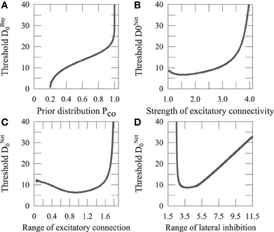
Figure 7. Threshold of integration. (A) The thresholds of the Bayesian model are plotted with the prior of sensory integration. (B) The thresholds of the network model are plotted showing the ratio of the strengths of the excitatory connection, M₁, and inhibitory connection, M₂, of the recurrent network. (C) The thresholds of the network model are plotted with the range of excitatory connection, σ₁. (D) The thresholds of the network model are plotted with the range of lateral inhibition, σ₂.

When the causal structure is defined, we can calculate the optimal estimate of the stimulus position for the cases of C = 1 and C = 2. When the audiovisual stimuli have independent causes, the optimal solutions are

$\begin{array}{cc}{\widehat{x}}_{V,C=2}=x_V,{\widehat{x}}_{A,C=2}=x_A.& (10)\end{array}$

When the audiovisual stimuli have a common cause, the optimal solution is

$\begin{array}{cc}{\widehat{x}}_{V,C=1}={\widehat{x}}_{A,C=1}=\frac{\frac{x_V}{{\sigma }_V^2}+\frac{x_A}{{\sigma }_A^2}}{\frac{1}{{\sigma }_V^2}+\frac{1}{{\sigma }_A^2}}.& (11)\end{array}$

We calculated the localization bias using the Bayesian model (Figure 6C). Here, we fixed P_co = 0.2, σ_V = 3 [deg], and σ_A = 6.5 [deg].

Both the Bayesian prior P_co and recurrent connectivity J_ij affect the integration threshold D₀. Thus, the integration threshold D₀ validates the idea that the Bayesian prior P_co corresponds to a recurrent connectivity J_ij in the cortical neural network.

4.3. Network Connectivity Represents Bayesian Prior P_co

Synaptic plasticity is thought to be the basic phenomena underlying learning. It could be said that a neural network learns a Bayesian prior by changing its connectivity. We investigated how the parameters of the network connectivity J_ij affect the integration threshold, as shown in Figure 7. D^Net₀ increases with the ratio between the strength of excitatory connection, M₁, and that of the inhibitory connection, M₂. It approximately increases with the range of excitatory connection, σ₁, similarly to the ratio between M₁ and M₂, whereas it varies with a non-monotonic shape for the range of lateral inhibition, σ₂, as illustrated in Figure 7D.

Let us focus on the excitatory connection that could be changed through Hebb's learning rule. As shown in Figures 7A, B, D^Net₀ increases with M₁ in the same way as D^Bay₀ increases with P_co. This means that the Bayesian prior P_co is represented as M₁ in the network model. This result suggests that the neural network achieves Bayesian inference through learning appropriate prior information by adjusting the excitatory connection M₁.

5. Discussion

We constructed a recurrent network model that distinguishes whether or not audiovisual stimuli have a common cause or distinct causes. We showed that our model not only estimates the number of sources, but also reproduces the localization bias, as observed in psychophysical experiments Wallace et al. (2004). Previous studies have revealed that the Bayesian ideal observer model could explain psychophysical data on sensory integration Körding et al. (2007); Sato et al. (2007). Although a Bayesian model gives a normative account of the computational principle, it does not provide a neural implementation of optimal causal inference. Our model is a biologically plausible one of cortical circuitry, and it provides information about how the nervous system can implement the computation Carandini et al. (1997). To reveal how the nervous system implements Bayes' inference, we investigated the relationship between the synaptic connection of the proposed model and the prior distribution in the Bayesian model. We found that the strength of the excitatory connection represents the prior distribution for the probability of integration.

Previous research has used divisive normalization for the firing rate, serving as a gain control. The network model extracted variables encoded by a population of noisy neurons Deneve et al. (1999). The neural activities converged to a smooth stable peak, and the position of the peak depended on the variables. Therefore, the position could be used to estimate these quantities in their model. Moreover, through proper tuning of the parameters, the model closely approximated the maximum likelihood, which would be used by an ideal observer in most cases of interest. However, two or more localized activities could not coexist in the previous network model. The model thus could not simultaneously estimate information about multiple sources, which is needed for living in a natural environment. We found that strong divisive normalization makes it hard for localized activities to coexist. Iteration of Equation 3 makes the ratio of local excitations large, and eventually, only the largest one can survive. This effect occurs if the exponent is greater than 1. We constructed a model in which an arbitrary number of local excitations could coexist by making the exponent equal to one. This simple normalization can be biologically implemented in a linear computation and shunting inhibition Carandini et al. (1997). Although our network may not achieve optimal inference for each source position, it is biologically plausible and can reproduce the properties of auditory-visual integration observed in psychophysical experiments. These results imply that normalization with a threshold linear function is important in multisensory integration with causal inference.

We reproduced the results of psychophysical experiments showing localization bias in audiovisual integration. Whenever stimuli were unified, the model estimated that the auditory position would shift to the location of the visual stimulus. This phenomenon is caused by the difference in the reliability of the stimuli. That is, because visual information for source localization is much more reliable than auditory information, vision dominates sound. Moreover, it is also known that when an auditory signal is more reliable than a visual signal, sound dominates vision Alais and Burr (2004). It is reported that localization bias is observed in some cross-modal cues Pavani et al. (2000). Our model represents the reliability of stimuli by the strength of the input activity. It can be generalized to other types of cue integration by changing the strength of the input activity.

The results of psychophysical experiments have been explained using Bayes' inference Körding et al. (2007); Sato et al. (2007). Bayes' inference is a method of reasoning that combines prior knowledge with current input data. In our brains, information about the external world is estimated on the basis of prior knowledge Doya et al. (2007). However, until now, it was unknown how prior knowledge can be represented in a neural circuit. We investigated how a neural network can implement prior knowledge. Our results suggest that neural networks learn an appropriate prior with synaptic plasticity.

In the Bayesian model, negative bias is assumed to be caused by sensory noise Körding et al. (2007); Sato et al. (2007). Stimuli are unified when the distance between the perceived locations of audiovisual stimuli which are shifted from their original positions is smaller than D^Bay₀; on the other hand, when it is larger than D^Bay₀, the stimuli are not unified. The averaged bias of the non-unified case takes on a negative value. In our neural network model, not only sensory noise but also the interaction of localized activities has an effect on the negative bias. Localized activities repel each other through the effect of a Mexican-hat type of connectivity (Figure 3). This corresponds to implementing the prior distribution such that of the likely positions of different input sources, which has not been implemented in the previous Bayesian models Körding et al. (2007); Sato et al. (2007). It is unclear where causal inference is performed in the brain. If the repulsive effect were to be observed in a brain region that performs multisensory integration, it would support the notion that our model is actually implemented in the brain.

Conflict of Interest Statement

The authors declare that the research was conducted in the absence of any commercial or financial relationships that could be construed as a potential conflict of interest.

References

Alais, D., and Burr, D. (2004). The ventriloquist effect results from near-optimal bimodal integration. Curr. Biol. 14, 257–262. doi: 10.1016/j.cub.2004.01.029

Pubmed Abstract | Pubmed Full Text | CrossRef Full Text

Amari, S. (1977). Dynamics of pattern formation in lateral-inhibition type neural fields. Biol. Cybern. 27, 77–87. doi: 10.1007/BF00337259

Pubmed Abstract | Pubmed Full Text | CrossRef Full Text

Bertelson, P., and Aschersleben, G. (1998). Automatic visual bias of perceived auditory location. Psychon. Bull. Rev. 5, 482–489. doi: 10.3758/BF03208826

CrossRef Full Text

Carandini, M., Heeger, D. J., and Movshon, J. A. (1997). Linearity and normalization in simple cells of the macaque primary visual cortex. J. Neurosci. 17, 8621–8644.

Pubmed Abstract | Pubmed Full Text

Deneve, S., Latham, P. E., and Pouget, A. (1999). Reading population codes: a neural implementation of ideal observers. Nat. Neurosci. 2, 740–745. doi: 10.1038/11205

Pubmed Abstract | Pubmed Full Text | CrossRef Full Text

Doya, K., Ishii, S., Pought, A., and Rao, R. P. N. (2007). Bayesian Brain: Probabilistic Approaches to Neural Coding. Cambridge, MA: MIT Press.

Hairston, W. D., Wallace, M. T., Vaughan, J. W., Stein, B. E., Norris, J. L., and Schirillo, J. A. (2003). Visual localization ability influences cross-modal bias. J. Cogn. Neurosci. 15, 20–29. doi: 10.1162/089892903321107792

Pubmed Abstract | Pubmed Full Text | CrossRef Full Text

Howard, I. P., and Templeton, W. B. (1966). Human Spatial Orientation. New York, NY: Wiley.

Hubel, D. H., and Wiesel, T. N. (1962). Receptive fields, binocular interaction and functional architecture in the cat's visual cortex. J. Physiol. 160, 106–154.

Pubmed Abstract | Pubmed Full Text

Körding, K. P., Beierholm, U., Ma, W. J., Quartz, S., Tenenbaum, J. B., and Shams, L. (2007). Causal inference in multisensory perception. PLoS ONE 9:e943. doi: 10.1371/journal.pone.0000943

Pubmed Abstract | Pubmed Full Text | CrossRef Full Text

Latham, P. E., Deneve, S., and Pouget, A. (2003). Optimal computation with attractor networks. J. Physiol. 97, 683–694.

Pubmed Abstract | Pubmed Full Text

Lewald, J., Ehrenstein, W. H., and Guski, R. (2001). Spatio-temporal constraints for auditory–visual integration. Behav. Brain Res. 121, 69–79. doi: 10.1016/S0166-4328(00)00386-7

Pubmed Abstract | Pubmed Full Text | CrossRef Full Text

Ma, W. J., Beck, J. M., Latham, P. E., and Pouget, A. (2006). Bayesian inference with probabilistic population codes. Nat. Neurosci. 9, 1432–1438. doi: 10.1038/nn1790

Pubmed Abstract | Pubmed Full Text | CrossRef Full Text

Marti, D., and Rinzel, J. (2013). Dynamics of feature categorization. Neural Comput. 25, 1–45. doi: 10.1162/NECO_a_00383

Pubmed Abstract | Pubmed Full Text | CrossRef Full Text

Pavani, F., Spence, C., and Driver, J. (2000). Visual capture of touch: out-of-the-body experiences with rubber gloves. Psychol. Sci. 11, 353–359. doi: 10.1111/1467-9280.00270

Pubmed Abstract | Pubmed Full Text | CrossRef Full Text

Pouget, A., Zhang, K., Deneve, S., and Latham, P. E. (1998). Statistically efficient estimation using population coding. Neural Comput. 10, 373–401. doi: 10.1162/089976698300017809

Pubmed Abstract | Pubmed Full Text | CrossRef Full Text

Sato, Y., Toyoizumi, T., and Aihara, K. (2007). Bayesian inference explains perception of unity and ventriloquism aftereffect: identification of common sources of audiovisual stimuli. Neural Comput. 19, 3335–3355. doi: 10.1162/neco.2007.19.12.3335

Pubmed Abstract | Pubmed Full Text | CrossRef Full Text

Shadlen, M. N., Britten, K. H., Newsome, W. T., and Movshon, J. A. (1996). A computational analysis of the relationship between neuronal and behavioral responses to visual motion. J. Neurosci. 16, 1486–1510. doi: 10.1016/0959-4388(94)90059-0

Pubmed Abstract | Pubmed Full Text | CrossRef Full Text

Shadlen, M. N., and Newsome, W. T. (1994). Noise, neural codes and cortical organization. Curr. Opin. Neurobiol. 4, 569–579.

Pubmed Abstract | Pubmed Full Text

Wallace, M. T., Roberson, G. E., Hairston, W. D., Stein, B. E., Vaughan, J. W., and Schirillo, J. A. (2004). Unifying multisensory signals across time and space. Exp. Brain Res. 158, 252–258. doi: 10.1007/s00221-004-1899-9

Pubmed Abstract | Pubmed Full Text | CrossRef Full Text