Extending stability through hierarchical clusters in Echo State Networks

Introduction

Echo State Networks (ESN) are a type of reservoir networks that have been demonstrated to be successful at predicating non-linear signals, especially those with strong spatiotemporal components (Skowronski and Harris, 2007; Tong et al., 2007; Verstraeten et al., 2007). Proposed by Jaeger (2001), they exploit a reservoir of analog units with random but fixed connections where training affects only weights that project from the reservoir to the output population units. This makes reservoir networks computationally cheap to train in comparison to methods such as backpropagation. The stability of ESNs is assured by fulfilling the echo state property, which ensures that the initial conditions are washed out at a rate independent of the input and prevents the accumulation of activity (Jaeger, 2001). Criteria for fulfilling the echo state property are outlined for a specific subclass of ESNs in Buehner and Young (2006) and for leaky integrator units (Jaeger et al., 2007).

Although their strength derives from the homogeneity of the reservoir and its ability to generate rich non-linear dynamics, the connectivity of ESN reservoirs is random and therefore sub-optimal. Previous reports investigated the idea of optimizing the network by modifying the reservoir connections, either by pruning connections (Dutoit et al., 2009) or training connections within the reservoir (Sussillo and Abbott, 2009). Other work has focused instead on modifying network architecture by either including a hierarchy of ESNs to extract features (Jaeger, 2007) or introducing reservoir substructures (Deng and Zhang, 2007; Xue et al., 2007). Both of the latter papers reported an improvement in performance against conventional ESNs for specific tasks with interesting additional properties: For the decoupled ESNs (DESN) presented by Xue et al., an input signal composed of sinusoidal terms was presented to a network where the reservoir consisted of laterally inhibited clusters. They observed that each cluster attenuated to a subcomponent of the input signal, improving performance. The Scale-Free Hierarchical ESNs (SHESN) of Deng and Zhang lack explicit decoupling and instead employ a hierarchically clustered reservoir architecture. These SHESNs perform better in predicting the Mackey-Glass sequence, which is often used as a benchmark for non-linear systems.

Deng and Zhang further noted that SHESNs appeared to be more robust to the choice of spectral radius as they remained stable for a larger range of spectral radius values. They observed stable behavior for ρ = 6, much higher than in similar ESNs that only displayed stable responses for ρ < 1. While this does not imply that the echo state property has been violated by increasing ρ > 1, it does, however, indicate that clustered ESNs may extend the range of permissible values for stable and transient states. In their report, only one set of reservoir parameters was examined for SHESNs and so how ρ varied with reservoir architecture was not quantified. Thus, it is unclear how the transition from a homogeneous reservoir to a hierarchically clustered network affects the stability of the system; in particular, is stability affected more by the presence of hierarchy or of clusters, or by a combination of both? Furthermore, is the transition from stable to unstable behavior independent of the degree of clustering and does the activity transition through an intermediate regime, such as those observed elsewhere (Ozturk and Principe, 2005)?

To address these issues, we use hierarchical ESNs (HESNs), a modified version of SHESNs, as a case study. We begin with a conventional ESN and introduce hierarchical clusters, charting how stability depends on both reservoir architecture and the spectral radius to determine the relative influence of each. To identify the relative contribution of clusters and hierarchy, we compare reservoirs that are clustered but lack hierarchy against those that have both.

Materials and Methods

Network Model

We first consider a generic ESN (Jaeger, 2001), which consists of an input population u, reservoir population x and output population y. These populations are coupled by connection weight matrices Wⁱⁿ for input to reservoir units, sparse connection matrix W^res for connections between reservoir units and W^out for reservoir to output units. Note that all matrices are directed, so generally W_ij ≠ W_ji. Additionally, ESNs can include feedback connections projecting from y back to x as well as connections directly from the input to output populations. Here, we chose to exclude both as we wanted to consider only the dynamics of the reservoir and their impact on the output population.

The governing equations, modified from the original description in Jaeger (2001), are given by

where f and g represent activation functions which are typically monotonic and bounded, such as sigmoidals. We chose both f and g as tanh and scaled and shifted the incoming signal from the input population in order to place it into the optimal operating range of the network. Here, the input signal always consisted of a sequence of impulses, each of unit amplitude. Noise n_a is added to the reservoir units in order to stabilize the network during the training process. Unless otherwise stated, noise was uniformly distributed for

The input and output populations were chosen to consist of 5 units each. The reservoir populations were set to be of size 50–1000 units (see following subsection for more details). These sizes were chosen for computational tractability. Connections in both Wⁱⁿ and W^res were randomly and independently assigned with connection probabilities conn_in and conn_res, respectively. The connectivities were set as Wⁱⁿ being fully connected with weights drawn with uniform probability from [−1, 1]. Since this study is concerned with reservoirs for feedforward ESNs, training was only performed for tasks where the output units were relevant, such as the calculation of memory capacity. As for all ESNs, Wⁱⁿ and W^res remain fixed for the duration of the network simulation so training, when performed, did not affect the structure of the reservoir.

Introduction of Hierarchy

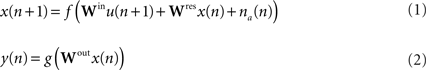
Different models of hierarchical networks exist which focus on different aspects of their structure: a clustered or modular architecture (Ravasz et al., 2002), existence of hubs (Sporns et al., 2007; Mueller-Linow et al., 2008), repetition of motifs across different scales (Ravasz and Barabasi, 2003; Sporns, 2006) or a combination of these features. For this study, we focus on a network model based on the SHESNs (Deng and Zhang, 2007), where sigmoidal units were replaced by ESN reservoirs. The resulting reservoir architecture differs from flat modular networks due to the presence of backbone units, which are units within a cluster that connect to backbone units in other clusters, in contrast to intracluster (local) units that only make connections within their own cluster (Figure 1A). Although no universally accepted definition of hierarchy exists, the majority of models examined in the literature focus on structures with a minimum of two levels of hierarchy. However, our aim was to establish the impact of hierarchy within a reservoir and contrast this effect against a structured but non-hierarchical architecture. Thus our modified SHESNs are minimally hierarchical networks, a property that is lost when the number of backbone units per cluster exceeds 1.

FIGURE 1

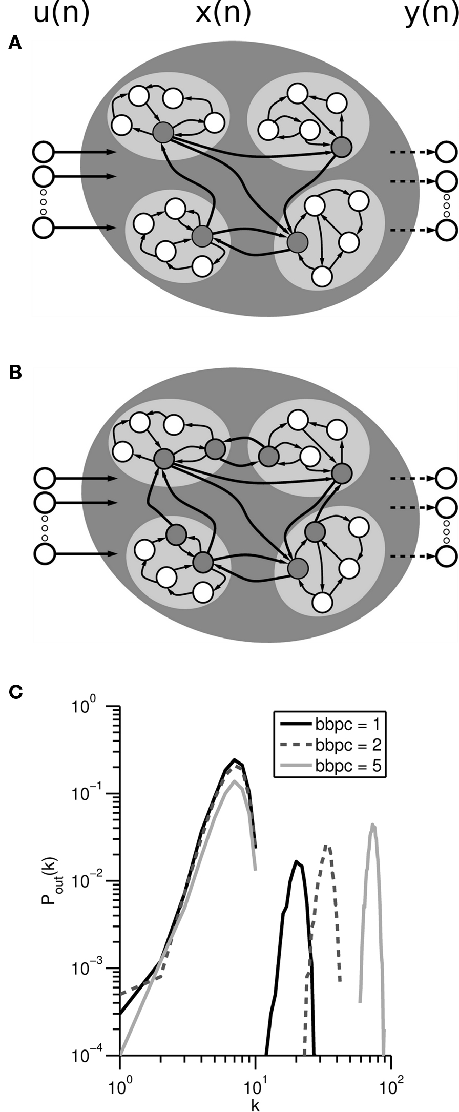
Figure 1. (A) Example of a HESN network with four clusters (light gray). Each cluster contains four local units (white circles) that only project within the cluster and one backbone unit (dark gray circles) that provide connections between clusters. Dashed lines indicate trainable weights. Each unit has a sigmoidal transfer function, bounded on [−1, 1]. (B) Non-hierarchical HESN with similar topology and two backbone units per cluster. By increasing the number of backbone units per cluster, the HESN becomes non-hierarchical and increasingly more homogeneous. (C) Average out-degree distribution P_out(k) for HESN with arbitrary configuration (200 units, 20 clusters, conn_inter = conn_intra = 0.7) against different values for backbone unit per cluster (bbpc), calculated over 50 independent realizations of reservoir. The connectivity does not follow a power law distribution and so is not scale-free, unlike the original SHESN model.

Four important changes were made in our networks as compared to the generation process outlined originally by Deng and Zhang to avoid some of the limitations present in their model with respect to the purpose of this case study: (1) Backbone units were originally detailed as being fully connected to one another. To enable us to decouple the intercluster and intracluster connectivities and examine the effect of varying them independently, we allowed the network of backbone units to have sparse connectivity; (2) To ensure that our network was topology independent, we did not assign a spatial location to the reservoir units; (3) To predetermine the network connectivities and cluster sizes, we kept the number of units per cluster constant within a network, using a seeding method outlined in more detail below; (4) To examine the transition from highly clustered to homogeneous architectures, we allowed more than one backbone unit per cluster which additionally allowed us to inspect non-hierarchically clustered networks (Figure 1B). These changes introduced three new parameters: intracluster connectivity conn_intra, intercluster connectivity conn_inter and number of backbone units per cluster bbpc.

The degree-distributions P_out(k) and P_in(k) (Albert and Barabási, 2002) followed a bimodal (Figure 1C) rather than the scale-free distribution observed for SHESNs. This can be attributed to our restriction of uniform cluster sizes and the fixed values for conn_intra and conn_inter. For this reason, we differentiate from SHESNs and instead refer to our model as hierarchically clustered ESNs (HESN).

A network was generated by first specifying the total reservoir size R, the number of clusters n, and the number of backbone units per cluster b. Each cluster was then created for size R/n and connectivity probability conn_intra, followed by the generation of the intercluster connectivity matrix. This was performed by identifying the first b units within each cluster as backbone units and then defining a matrix of size (bR/n) with connection probability conn_inter. The connectivity weights were drawn randomly from a uniform probability on [−1, 1]. The connectivity matrix of the reservoir W^res was then rescaled to set the largest eigenvalue to be equal to the defined spectral radius.

To establish the effect of reservoir size on cluster configuration, we defined several configurations of cluster number and size while keeping the total number of units within the reservoir constant. Reservoir size was limited to 1000 units for computational tractability. Note that a conventional ESN is obtained when cluster size is equal to either 1 or the total reservoir size. As a default configuration for HESNs, we assumed bbpc = 1 and conn_inter = conn_intra = 0.7. Connection probabilities were always incremented in steps of 0.05. bbpc was generally set to be multiples of 5, except if cluster size was below 10. In these instances, all possible values for bbpc were tested. These additional criteria allowed us to manipulate the reservoir structure and independently vary its degree of hierarchy and clustering. Importantly, we were able to test hierarchically clustered reservoirs against non-hierarchically clustered reservoirs by retaining a fixed total number of intercluster connections while changing their distribution. This was possible by specifying a larger number of backbone units per cluster and then decreasing the intracluster connectivity to compensate.

In conventional ESNs, the largest eigenvalue of W^res (spectral radius ρ) is used as an indicator of stability of network dynamics. Traditionally, ρ less than unity is sufficient for zero-input networks to ensure stable dynamics; Buehner and Young (2006), however, outlines an additional criterion necessary to ensure stability, as stability is also observable for ESNs when ρ > 1 (Ozturk and Principe, 2005; Verstraeten et al., 2007). We examined the effect of increasing ρ on stability and during our simulations the spectral radius was varied from 0.05 to 2 in increments of 0.05. For each cluster configuration, we determined ρ_max, which we defined as the largest permissible ρ for which the network remained stable under the criteria outlined in the following subsection.

Identification of Network Behavior

Different possibilities exist for characterizing a specific reservoir configuration (see Lukosevicius and Jaeger, 2007; Schrauwen et al., 2007 for discussion). Of specific interest to us was how sensitive the system was to noise and how reproducible its dynamics were. Here, we considered an approximation of the maximal Lyapunov exponent to determine stability, and the distribution of reservoir activity values upon multiple stimulation with the same sparse stimulus to assess reproducibility. We also calculated the network memory capacity to provide a measure for the functional performance.

A measure of stability is the Lyapunov exponent λ, which relates the divergence Δ between two trajectories after introducing a small perturbation δ to the elapsed time via Δ = e^λt. For stable systems, the deviation between the two trajectories should converge to 0, corresponding to a negative Lyapunov exponent. The existence of a positive Lyapunov exponent signifies that the trajectories exponentially diverge from each other with time, indicating that the system is sensitive to initial conditions and is thus likely to be chaotic. While the Lyapunov exponent cannot be easily calculated analytically for non-autonomous systems, different approaches for determining approximations of Lyapunov exponents for reservoir networks have been outlined, either based on experimental observation of a trajectory’s divergence following a perturbation (Skowronski and Harris, 2007) or theoretically by considering the deformation of an infinitesimally small hypersphere as the center follows a trajectory (Verstraeten et al., 2007). Here, we implemented an approximate numerical method, using the former approach (Wolf et al., 1985; Skowronski and Harris, 2007) and estimated the pseudo-Lyapunov exponent by introducing a perturbation δ to the reservoir state at time t_δ. Two identical networks, f and p, were created and driven with identical input and n_a = 0. At t_δ, only the second network p was perturbed, after which the simulation continued to run until t_end. The resulting divergences was then measured as the Euclidean 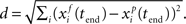distance The Lyapunov exponent was calculated as The networks were always driven by input consisting of a train of impulses, whose average rate was set to be equal to the rate used for the reservoir activity distribution task below. The perturbation δ was applied to the entire reservoir state, uniformly distributed with |δ| = 10⁻⁶ with t_end = 100 timesteps. As this technique does not lend itself to estimating the Lyapunov exponent by combining estimates of the same system (Wolf et al., 1985), we classified each network configuration by calculating the Lyapunov exponent for 100 independent realizations and determining the mean.

To relate this somewhat abstract notion of stability to a quantitative description of reservoir dynamics, the distribution of reservoir activity values in response to a sparse stimulus was also considered. This was determined by first defining a stimulus consisting of fixed pattern of input impulses presented multiple times at a constant interstimulus interval of either 10, 50, 100, or 1000 timesteps. We calculated the total reservoir activity for each timestep and normalized it by the number of reservoir units before computing the mean and standard deviation. This was repeated for 100 independent realizations of the same network configuration with n_a = 0.

The memory capacity MC for different HESN configurations was determined by presenting input signals to the network to be reproduced with increasingly longer delays between presentation and retrieval. MC is obtained by summing the correlation coefficient between the output signal and the input signal for each delay k, MC = Σ_k=1MC_k, where 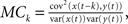as described in Jaeger (2002) and Verstraeten et al. (2007). Here, we calculated MC for k = 1–20 timesteps for an input signal consisting of train of exactly one delta input present at each timestep, distributed equally across all five input channels.

Results

The aim of the current study was to establish the impact of reservoir substructures – particularly hierarchical clustering – on the stability of ESNs. We begin by analyzing the effect of hierarchical clustering within reservoirs for a fixed spectral radius, considering underlying factors such as the number of backbone units per cluster and intercluster connectivity. We then test whether clustering by itself is sufficient to alter the upper bound of permissible values for the spectral radius. Lastly, we consider the memory capacity for various network configurations.

Impact of Clusters on Stability

We aim to determine the effect of hierarchical clustering on the limits for spectral radius values for stability and began by systematically examining the impact of cluster on dynamics for different cluster configurations while the spectral radius remained constant. We considered a simple HESN with a fixed ρ = 1.2, conn_inter = conn_intra = 0.7 and assumed only one backbone unit per cluster.

Various network configurations were examined by first fixing the total reservoir size and then increasing the number of clusters (Table 1). We determined the reservoir activity distribution, using very sparse input sequence repeated every 50 timesteps, and observed three response types across all simulations: (i) the network showed some activation, but this quickly died with exponential decay (Figure 2A). The corresponding reservoir activity values had both low mean and low standard deviation. (ii) The network either never stabilized or was unstable after the presentation of the first stimulus (Figure 2C), with large mean reservoir activity values with low standard deviation; or (iii) transient behavior, which was similar to stable behavior except that the reservoir activity does not return to 0, but rather to some non-zero baseline activity (Figure 2B). Although the non-zero baseline remained more or less constant within a trial, its value varied between trials, leading to a standard deviation of normalized reservoir activity values that was far higher than of either stable or unstable reservoirs, where the standard deviation of reservoir activity was <0.05.

TABLE 1

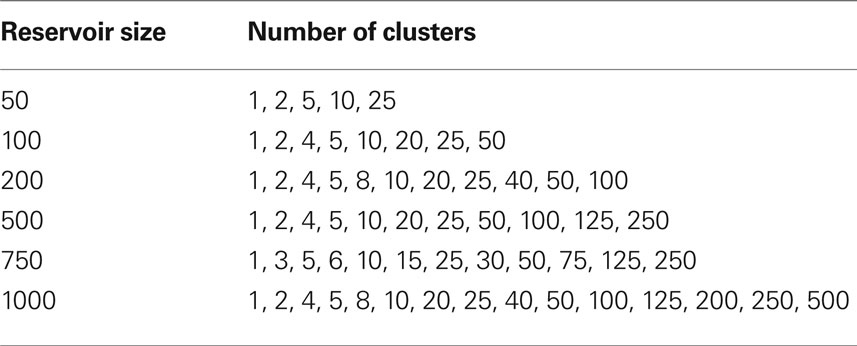
Table 1. Cluster configurations tested for different reservoir sizes.

FIGURE 2

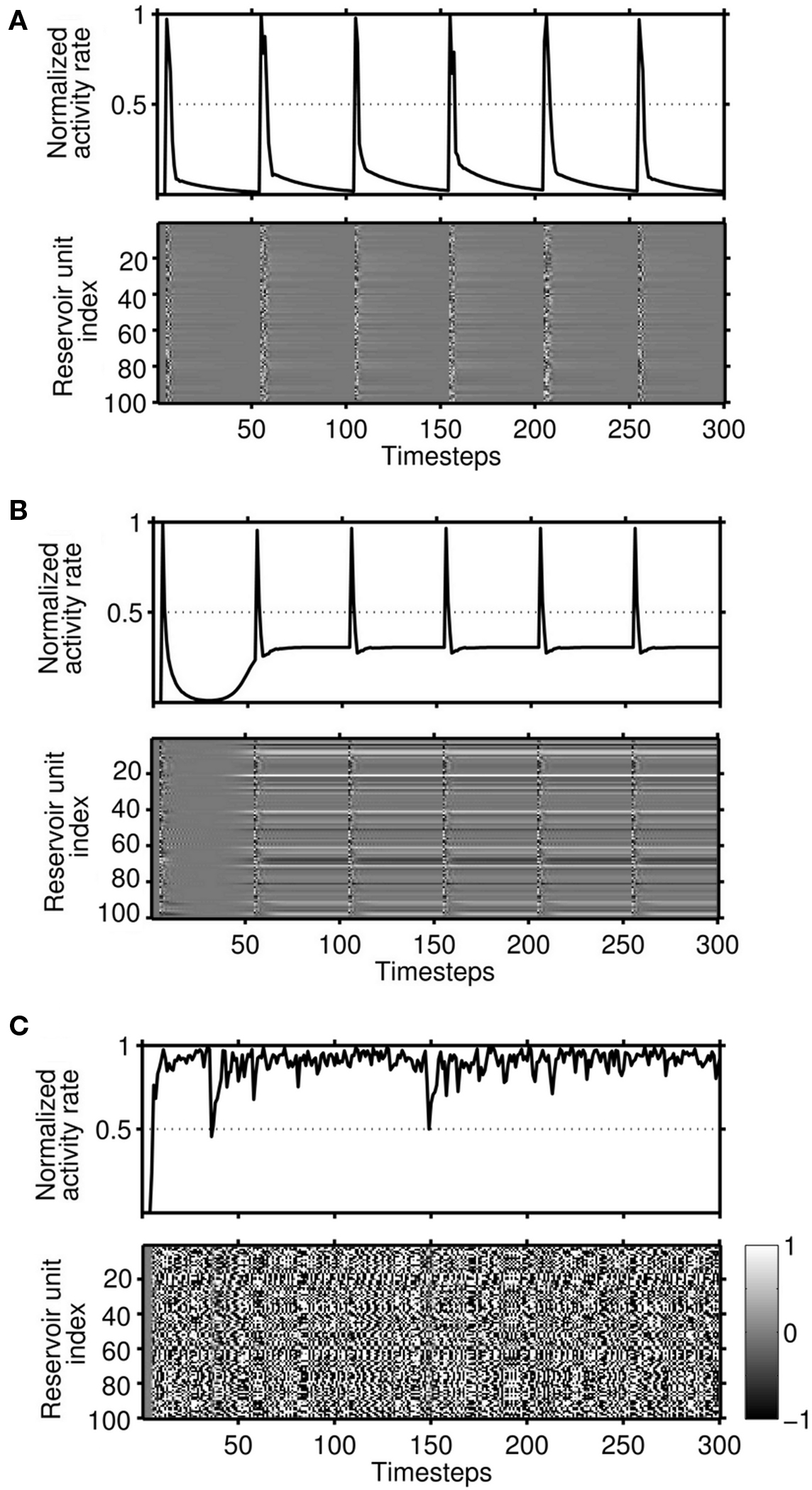
Figure 2. Responses of reservoirs to a repeated stimulus pattern for networks with R = 100 and different values of ρ. (A) For n = 2 clusters, stable dynamics occur where responses fade within a highly reproducible and fixed time-period, illustrating that the dynamics are input driven only. Shown is for both the normalized total activity rate (top) and reservoir activity (bottom). (B) With n = 20, transient dynamics were similar to stable but were characterized by activity decaying to a non-zero baseline. Baseline activity values for identical network configurations displayed high variability across trials. (C) Unstable dynamics for n = 50, where the system never returns to zero activity after the first input.

The stability of a network did not depend on absolute reservoir size, absolute cluster size or the number of clusters alone, but rather on the combination of these factors (Figures 3A,B). Unstable responses occurred in large networks with a small number of larger clusters, while stable responses were observed for configurations with smaller clusters. Transient responses occurred in a broad region between stable and unstable responses and for configurations of intermediate cluster size.

FIGURE 3

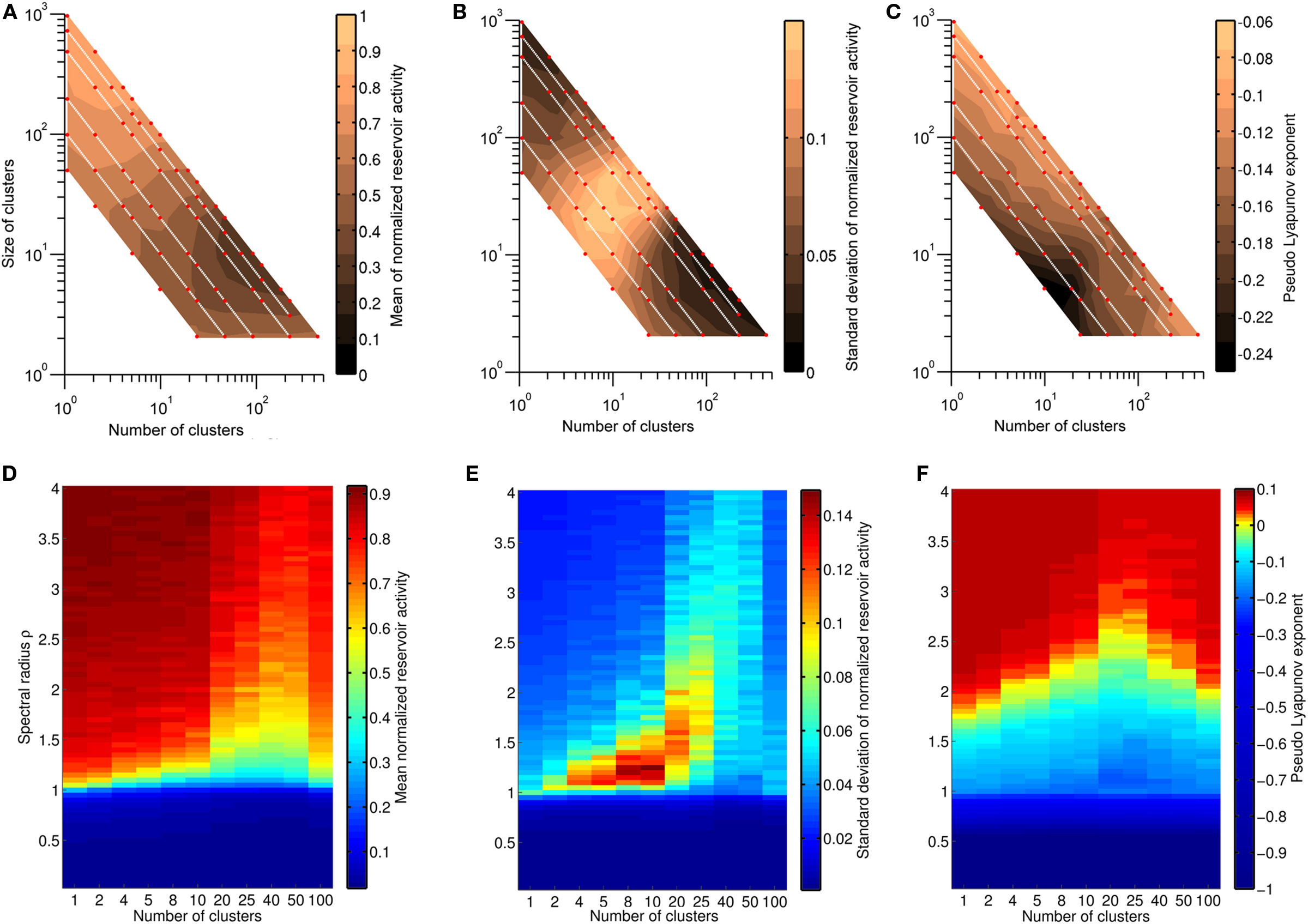
Figure 3. (A–C) Six different reservoir sizes were examined (R = 50, 100, 200, 500, 750, 1000) with varying number of clusters. All other network parameters were kept constant with ρ = 1.2, conn_intra = conn_inter = 0.7, and bbpc = 1. Mean and standard deviation of normalized reservoir activity (A,B) were determined for 100 realizations of each network configuration, with red dots indicating the location of each network configuration in parameter space and white lines indicating networks with identical reservoir size. The area between tested network configurations was interpolated to visualize the trend. Unstable responses are characterized by a high value for the mean reservoir activity and occurred for networks with a small number of large clusters. Transient responses can be distinguished by large fluctuations of normalized reservoir activity, while stable responses have low mean activity. The same network configurations were also used to calculate the pseudo-Lyapunov exponent (C). Negative values were observed for all networks, indicating that networks tested were non-chaotic. (D–F) Distributions of normalized reservoir activity values and the pseudo-Lyapunov exponent were calculated as the spectral radius ρ was varied between 0.05 and 4 in HESNs for R = 200 with different cluster configurations. ρ_max increased with increasing number of clusters up to n = 40, while the region of networks that generate transient responses also increases with increasing n.

The pseudo-Lyapunov exponent was also calculated for the same set of network configurations (Figure 3C). Only negative values were observed, indicating that all configurations were non-chaotic for ρ = 1.2. However, the magnitude of the exponent varied and revealed that configurations of intermediate cluster size had the lowest value for . This result also demonstrates that the responses of networks with a negative maximum pseudo-Lyapunov exponent do not necessarily decay to 0, and that ongoing activity in feedforward ESNs (Figures 2B,C) does not necessarily imply a chaotic regime.

To examine how these trends for stability and chaoticity developed as the spectral radius increased, we analyzed different cluster configurations for a HESN with a fixed reservoir size and considered both distribution of reservoir activity values and the largest pseudo-Lyapunov exponent (Figures 3D–F). We set R = 200 and kept all other parameters identical to those used in the previous task, but increased ρ from 0.05 to 4 in 0.05 increments. Our results clearly demonstrate that both the mean reservoir activity value and the pseudo-Lyapunov exponent were lower for the same spectral radius value when clusters were present, with the lowest values occurring for reservoirs with 20–50 clusters. This confirms that the addition of hierarchical clusters extends the permissible range of spectral radius values and is consistent with the trend observed in Figure 3C, with cluster configurations of intermediate size displaying the largest range of negative Lyapunov exponents.

Increasing the input population from 5 to 50 units for bbpc = 1 led to more network configurations with unstable responses (not shown), corresponding to an extension of the region of instability in Figure 3A toward networks with a larger number of clusters. We hypothesize that the larger input population provides more activation to the reservoir, which saturates network activity. Thus, networks with larger clusters are able to resist network activity saturation better than networks with smaller clusters.

Spectral Radius Range

To establish the effect of other network parameters on the range of permissible spectral radius values, we determined the maximal spectral radius value that resulted in a negative pseudo-Lyapunov exponent ρ_max for three different parameters related to reservoir architecture: reservoir size R, the number of backbones per cluster bbpc and intercluster connectivity conn_inter.

To determine how the span of ρ for stable networks was affected by total reservoir size, the simulation was repeated for R = 100, 200, and 500 (Figure 4A). As the reservoir size increased, ρ_max strongly decreased. The location of the peak value for ρ_max, however, remained relatively constant when plotted against relative cluster size (n/R) and occurred for clusters sizes 2–5% of the total reservoir size.

FIGURE 4

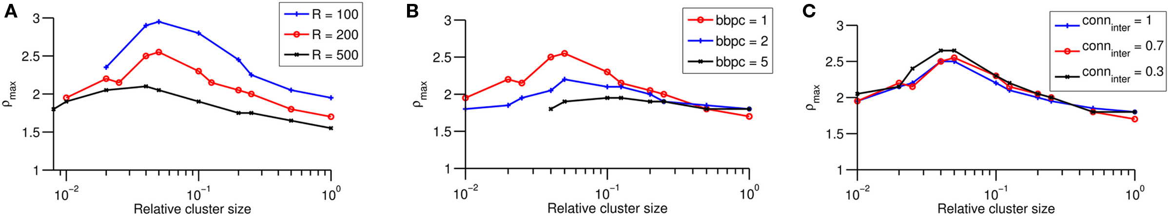
Figure 4. (A–C) Range of ρ_max as a function of relative cluster size for three different reservoir sizes (A), different number of backbone units per cluster (B) and different intercluster connectivities (C). (A) Increasing the reservoir size decreases ρ_max, while the location of the peak value remains unchanged. (B) Increasing bbpc drastically decreases the peak value of ρ_max, while (C) decreasing conn_inter only slightly increases ρ_max across different relative cluster sizes. Note that the default network configuration for this task is signified by red in all plots.

Increasing the number of backbone units per cluster makes the reservoir more homogeneous, which should have a greater impact on the spectral radius range for networks with smaller clusters. Increasing the number of backbone units per cluster to bbpc = 5 for R = 200 (Figure 4B) yielded a decrease in ρ_max and caused the distribution to become progressively more uniform. The location of the peak value for ρ_max appeared to remain unchanged for bbpc ≤ 2. To test whether increasing bbpc affects reservoir activity and the pseudo-Lyapunov exponent, we examined the various size networks previously tested using a fixed ρ = 1.2 and bbpc = 5 (Figures 5A–C). We observed that many previously stable networks now displayed higher values for both mean reservoir activity and the pseudo-Lyapunov exponent, confirming that this effect was a general property of increasing bbpc.

FIGURE 5

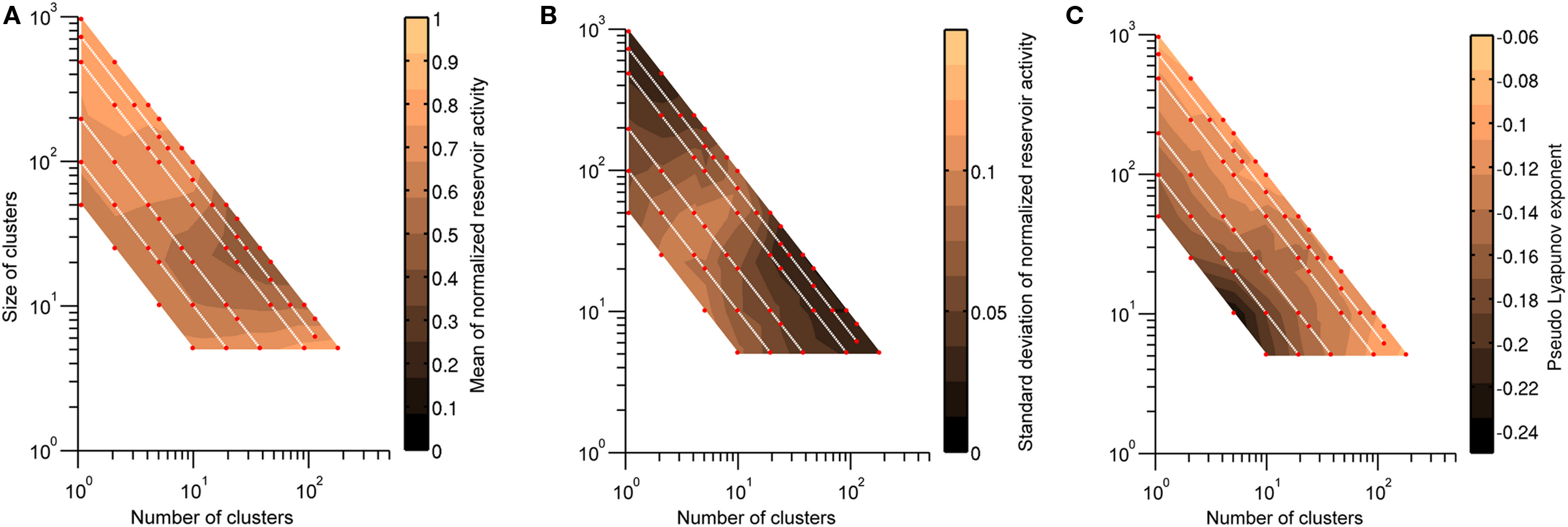
Figure 5. Mean and standard deviation of normalized reservoir activity values (A,B) and the pseudo-Lyapunov exponent (C) when the number of backbone units per cluster bbpc is increased to 5. This leads to an increase in the number of configurations with unstable responses. Details as for Figure 3.

It has been observed for ESNs that sparser connectivity results in lower error rates. If we treat each cluster as being comparable to a single unit within an ESN reservoir, then the performance of HESNs should increase with lower intercluster connectivity conn_inter. Since high performance requires stable network configurations, we expect some dependence of ρ_max on conn_inter. Our findings reflect this, with ρ_max increasing for network configurations with larger numbers of clusters as conn_inter was decreased (Figure 4C). The location of peak ρ_max at n = 20, however, remained unchanged by decreasing conn_inter.

As varying the spectral radius only changed the values but not the structure of the distribution of eigenvalues, we expected that any change in ρ_max for increasingly clustered networks is likely due to differences in the eigenvalue distribution, rather than the spectral radius itself. We therefore analyzed the eigenvalue spectra of 20 realizations of each cluster configuration previously examined. Eigenvalue spectra for configurations with a small number of clusters were homogeneous (Figure 6A), similar to those obtained for ESNs. The spectra became increasingly more focused around the origin as clustering was increased (Figure 6B). However, the eigenvalue spectra partially dispersed again for reservoirs with a high number of clusters, e.g., n = 500, and appears similar to Figure 6A, but now with approximately 40% of the eigenvalues located at the origin. The distribution of eigenvalues sorted by distance from the origin summarizes this for all cluster configurations (Figure 6C). The distributions increasingly deviated from a homogeneous distribution as the number of clusters increased, due to the progressively more significant contribution of the intercluster connections.

FIGURE 6

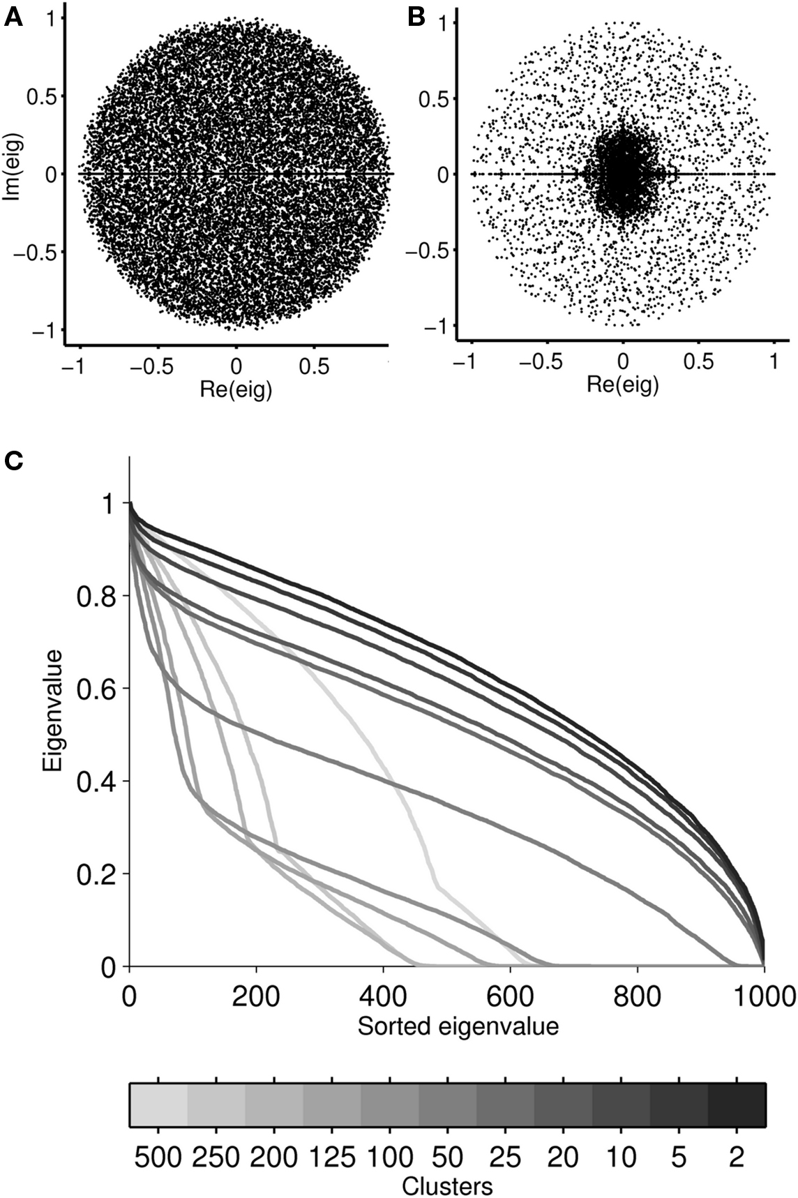
Figure 6. Eigenvalue spectra for 20 realizations of a reservoir with R = 1000 and 2 clusters (A) or 125 clusters (B). To visualize how the distribution of eigenvalues varied as clustering was increased, eigenvalues were sorted by their distance from the origin and plotted for ρ = 1 (C), with each curve representing the mean of 20 realizations for each cluster configuration. Reservoirs with n > 25 have a non-uniform eigenvalue distribution with more than 30% of their eigenvalues concentrated at the origin.

Hierarchical Clusters

Hierarchy is determined by the degree distribution while clustering is determined by the degree count. To establish the relative influence of each on network dynamics, we compared four network configurations with varying bbpc and conn_inter values. Specifically, we chose values for both parameters that would lead to identical degree counts but different degree distributions (Table 2).

TABLE 2

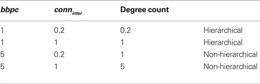
Table 2. Network configurations tested for the effect of varying both intercluster connectivity conn_inter and number of backbones per cluster bbpc. Degree count is calculated as the product of bbpc and conn_inter.

Our results in the previous section demonstrate that ρ_max is decreased by increasing bbpc (Figure 4B) or decreasing the intercluster connectivity. These trends were confirmed while testing the degree counts of networks (Figure 7). While we observed no significant difference for reservoirs with five clusters or less, as the number of clusters increased, so did the difference between ρ_max for hierarchical and non-hierarchically clustered networks. The range of ρ_max was higher for the hierarchically clustered networks than for the non-hierarchically clustered networks. We can conclude therefore that it is the degree distribution and thus hierarchy, rather than degree count and clusters, that exerts the larger influence on the range of ρ_max.

FIGURE 7

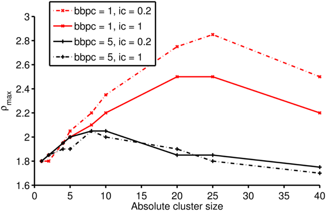
Figure 7. ρ_max for increasing number of clusters for four different combinations of values for bbpc and conn_inter. The corresponding increases in ρ_max are consistent with trends described above. The relative influence of hierarchy and clustering can be observed by considering the two networks with the same degree count but different distributions: bbpc = 1, conn_inter = 1, and bbpc = 5, conn_inter = 0.2. For n > 5 clusters, the former configuration has higher values of ρ_max, indicating a greater dependence of ρ_max on hierarchy rather than clustering.

Memory Capacity

So far, we considered only measures related to the stability using measures related to reservoir dynamics. To reconcile the affect of clustering with measures related to the performance of a ESN, we calculated the memory capacity MC of HESNs while varying the number of clusters n, intercluster connectivity conn_inter, and bbpc separately to establish their individual influence as ρ is increased (R = 200, conn_intra = conn_inter = 0.7, and bbpc = 1, unless otherwise specified). For each network configuration, MC was calculated as the mean of twenty independent realizations.

The cumulative memory capacity was determined for increasing delays t from 1 to 20 while ρ was fixed at 0.7 (Figure 8). MC increased with decreasing the number of clusters, with a maximum of 8.04 for n = 1. The higher plateau level indicates that there was no contribution to MC for delays higher than 10 timesteps.

FIGURE 8

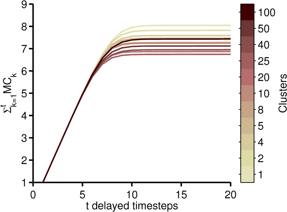
Figure 8. was calculated for a collection of clustered reservoirs with total reservoir size R = 200 and for delay t ranging from 1 to 20 timesteps.

We examined the effect of varying bbpc and conn_inter for four cluster configurations with n ≤ 40 to ensure we could use the same cluster configurations with bbpc = 5. Based on curves obtained for Figure 8, we selected n = 1, 5, 25, and 40 as a representative cross-section. For 0.05 ≤ ρ ≤ 4 using bbpc = 1, 2, and 5 and the cluster configurations as described above (Figure 9A), increasing bbpc had no difference for networks where n ≤ 5. The effect of increasing bbpc, however, was most obvious for networks with larger n, with the maximum MC increasing from 7.4 (bbpc = 1) to 9.8 (bbpc = 5) for n = 40. Overall, increasing bbpc led to a more homogeneous distribution of MC values, reflecting that a network with n = 1 can be approximated by networks with high n and high bbpc values.

FIGURE 9

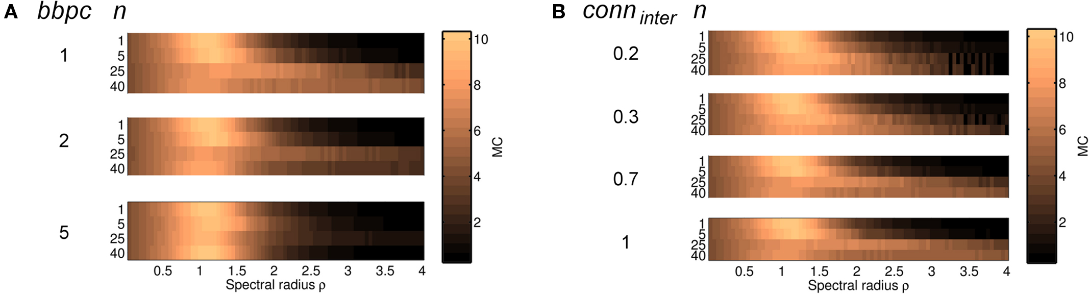
Figure 9. MC was calculated for four different cluster configurations as ρ was increased from 0.05 to 4 (R = 200, conn_intra = 0.7 with conn_inter = 0.7 and bbpc = 1, unless otherwise stated). The effect of increasing bbpc (A) and varying conn_inter (B) was most noticeable for networks where n ≥ 25 where MC was high over a broader range of ρ.

MC was compared for conn_inter = 0.2, 0.3, 0.7, and 1, which were chosen for comparison with previous simulations. Here we examined MC across the four cluster configurations with ρ increasing from 0.05 to 4 in increments of 0.05 (Figure 9B). MC was maximal for both n = 1 and 5 when ρ was slightly larger than 1. As expected, MC was independent of conn_inter, since conn_inter has little to no influence in networks with few clusters. While MC was low in networks with n = 25 and 40, their MC was also maximal for ρ > 1 but, importantly, decreased as conn_inter increased. This is likely because intercluster connections became more significant as the number of clusters increased and thus the dominance of intracluster connections decreased in favor of intercluster connections.

Discussion

ESNs with structured reservoirs have been suggested to perform better in predicting non-linear signals (Deng and Zhang, 2007; Xue et al., 2007). Furthermore, clustered reservoirs appear to extend the range of permissible spectral radius values and result in more robust reservoir networks. Our results demonstrate that the addition of clusters within a reservoir does increase the range of spectral radius values that can be chosen, but that this increase does not occur uniformly. Specifically, we charted how the upper limit for the range of the spectral radius ρ that resulted in stable dynamics depended on the reservoir structure and showed: (1) ρ_max varied with the number and size of clusters; (2) the range of ρ_max was flattened as the number of backbones per cluster was increased and the reservoir becomes more homogeneous; (3) decreasing the intercluster connection probability conn_inter increased ρ_max but did not affect the location of the peak value for ρ_max. These findings demonstrate that several factors interact to set the upper limit for spectral radius within HESNs. As we could examine only a small subset of all possible combinations of parameter values, however, varying multiple parameters simultaneously may have unpredicted effects on reservoir dynamics.

The criterion for stability within ESNs is that the echo state property is fulfilled; for purely feedforward ESNs, ρ < 1 is a sufficient but not necessary condition as it ensures that the eigenvalues are scaled such that the system always contracts for any possible input (Jaeger, 2001). This property is evident in our plots, as the estimated Lyapunov exponent and the activity levels are independent of clusters when ρ < 1. However, increasing ρ beyond 1 does not directly violate the echo state property and there has been recent interest in methods to identify the upper bound (Buehner and Young, 2006). As our results and those from others (i.e., Ozturk and Principe, 2005; Verstraeten et al., 2007) demonstrate, it is easily possible to choose ρ to be larger than 1 and still avoid unstable states. Understanding the interaction between different structural properties should assist in the identification by quantifying bounds for the spectral radius for different reservoir structures, although we were unable to determine a universal criterion for the echo state property in the networks we examined,

In homogeneous ESNs, larger ρ values result in a slower decay of the network’s response to an impulse (Jaeger, 2001) and strongly affect performance (Venayagamoorthy and Shishir, 2009). It is thus important to choose ρ appropriately. For example, a HESN with 200 units and four clusters was unstable when ρ = 1.2, but was stabilized when the number of clusters was increased. Thus, configurations that would previously have been dismissed due to instability can now be reconsidered, allowing greater flexibility in the design of clustered reservoirs. We were also able to demonstrate that the presence of clusters is reflected in the memory capacity MC. Clustered reservoirs displayed lower peak MC values; importantly however, MC values decreased more slowly as ρ increased for clustered reservoirs when compared to non-clustered reservoirs for ρ > 1.5. These factors together imply that clustered ESNs are more robust over a broader range of spectral radius values than traditional ESNs.

We were also able to map the transition between stable to unstable responses through an intermediate regime, where the reservoir activity decayed to a non-zero baseline after the first stimulus was presented, resembling the transient activity identified by Ozturk and Principe (2005). The baseline of reservoir activity was generally constant for each realization of an HESN. For all reservoir configurations, the mean reservoir activity increased as ρ grew larger. The level of ongoing activity can be thought of as corresponding to the elasticity of the system: as the ongoing activity increases, the potential energy of the system decreases. The gradient at which this transition to instability occurs as the spectral radius is increased, therefore, greatly affects the maximal spectral radius that can be chosen. Our findings indicate that this transition was slowest for 40–50 clusters in reservoirs with 200 units (Figures 4D,E), which is reflected in the slow decrease in MC for the corresponding network configurations.

Effect of Hierarchical Clusters on Dynamics

One question raised implicitly following the original observation of an extended range of ρ_max was whether it was increased by the introduction of hierarchy, or whether merely a clustered topology was sufficient. As hierarchically clustered reservoir are characterized by having only one backbone unit per cluster, we compared hierarchically clustered reservoirs against cluster configurations that had the same number of intercluster connections that were, however, distributed over more than one backbone unit per cluster. Our findings indicate that, while the choice of cluster configuration does influence the value of ρ_max, the range of spectral radius values for stable ESNs is affected more by the distribution of intercluster connections onto cluster units, rather than their number. Therefore, we conclude that the presence of hierarchy, rather than clustering per se, is responsible for the extended range of permissible ρ values.

This characteristic is likely due to the ability of hierarchically clustered networks to reduce the impact of unstable behavior: if one cluster becomes unstable, its influence on other clusters is minimized by a low number of backbone units, which act as bottlenecks. This behavior has been observed for tri-state networks (Kaiser et al., 2007). Consistent with this, increasing the number of intercluster connections decreased network stability. This is supported by analysis of reservoir unit activity traces in networks with transient responses, where the activity trace showed one cluster that was strongly active.

One question of special interest was whether there was “golden ratio” of cluster sizes: Given a total reservoir size, is there an optimal cluster size for that will maximize ρ_max? For the reservoir sizes we examined, the configuration that resulted in the maximal ρ_max for R = 200 was 25 clusters of 8 units each, corresponding to cluster sizes of 4% of reservoir size. For R = 100 and 500, these values were 20 clusters of 5 each (5%) and 50 clusters of 10 units (2%), respectively. These results suggest that cluster sizes of 2–5% of the total reservoir size are optimal. The benefit of having such small cluster sizes can be seen by considering a network with only a few large clusters: if one cluster becomes unstable, the instability of that cluster drives the baseline activity rate higher, reducing the elasticity of the reservoir. As successive clusters become unstable, the baseline rises and the computational potential of the reservoir decreases. For large cluster sizes, this increase happens quite quickly; in contrast, the loss of a small cluster results in smaller increments and therefore a slower transition to instability. Importantly, this interpretation holds true only when clusters have little impact on the activity of other clusters and so is only observed in hierarchically clustered networks, due to the presence of bottlenecks which allow the HESN’s performance to degrade gracefully.

Quantifying ESNs

One problem that has often been discussed is how to measure the “goodness” of a given ESN (Lukosevicius and Jaeger, 2007). While more primitive measures, such as the error rate, can be easily applied, they are task dependent and therefore highly subjective. Most importantly, they do not supply any additional information as to how the reservoir structure impacts on performance. Other measures that examine reservoir activity, such as cross-correlation of reservoir unit activity or entropy of reservoir states (Ozturk et al., 2007), have been used to relate performance to reservoir dynamics. Here, we used the normalized reservoir activity, a metric based on mean reservoir activation following a sparse input applied at a fixed frequency. While this measure has limited use, it was well-suited to indicate the level of ongoing activity, which was of particular interest to us.

A more sophisticated measure is the Lyapunov exponent, which indicates how chaotic a system is. However, this measure has strong shortcomings associated with it. Generally, Lyapunov exponents are difficult to estimate for non-autonomous systems, such as stable feedforward ESNs, which must be externally driven. Correspondingly, any estimate of the Lyapunov exponent is sensitive to the input used, making generalization difficult. On the other hand, there is no clearly better method to estimate the Lyapunov exponent: while the theoretical approach used by Verstraeten et al. (2007) allows for simultaneous consideration of all trajectories in the vicinity of the operating point, it can only estimate positive Lyapunov exponents. As we explicitly wanted to observe how quickly a network configuration moved from stable to chaotic behavior, we chose to approximate the Lyapunov exponent numerically. However, the disadvantage of numerically approximating the Lyapunov exponent is that it is inexact and time-consuming to calculate. Furthermore, determining the Lyapunov exponent by applying a reservoir perturbation is also subjective to the magnitude of the applied perturbation. We were able to demonstrate that for perturbations both two orders of magnitude larger and smaller than δ = 10⁻⁶, the same dependency of stability on the number of clusters was still present and with the same structure. This observation allows us to conclude that, although the location of the transition to a chaotic regime depends on input and perturbation magnitude, reservoir stability remains strongly determined by not only the presence but also the size of clusters within the reservoir.

Conclusion

The total reservoir size, number of clusters, backbone clusters per unit, and intercluster connectivity all affect the range of permissible spectral radius values and we demonstrated that their interplay determines the upper boundary for the spectral radius. Specifically, the range of permissible spectral radius values strongly depended on the ratio of cluster size to total reservoir size. Hierarchy, rather than clustering alone, had the largest impact on the range of spectral radius values for stable networks. Furthermore, increasing the intercluster connectivity extended the range of spectral radius values for stable ESNs, while increasing the number of backbone units per cluster had the opposite effect.

The transition from stable to unstable dynamics was characterized by responses with varying levels of ongoing activity, even in the absence of any stimulus. The amount of ongoing activity increased as the spectral radius was raised, leading to progressively more unstable reservoir dynamics. Importantly, the rate at which this transition occurred was slowest for hierarchically clustered reservoirs with clusters of size in the range 2–5% of the total reservoir size. We suggest that this is due to backbone units acting as bottlenecks that partition the reservoir, which minimizes the influence of any unstable units by limiting their impact to their own cluster. This effect is optimal when clusters sizes are small enough that the loss of any single cluster does not greatly affect the overall reservoir dynamics, leading to a graceful degradation of reservoir performance, but large enough for them to still contribute to reservoir dynamics. We conclude that hierarchy is a crucial feature for extending the range of permissible spectral radius values within feedforward ESNs.

Conflict of Interest Statement

The authors declare that the research was conducted in the absence of any commercial or financial relationships that could be construed as a potential conflict of interest.

Acknowledgments

We would like to thank H. Jaeger for extensive and valuable feedback and T. Gürel for helpful comments and discussion. This work was supported by the German BMBF (FKZ 01GQ0420, FKZ 01GQ0830) and by the EC (NEURO, No. 12788).

References

Albert, R., and Barabási, A.-L. (2002). Statistical mechanics of complex networks. Rev. Mod. Phys. 74, 47–97.

CrossRef Full Text

Buehner, M., and Young, P. (2006). A tighter bound for the echo state property. IEEE Trans. Neural Netw. 17, 820–824.

Pubmed Abstract | Pubmed Full Text | CrossRef Full Text

Deng, Z., and Zhang, Y. (2007). Collective behavior of a small-world recurrent neural system with scale-free distribution. IEEE Trans. Neural Netw. 18, 1364–1375.

Pubmed Abstract | Pubmed Full Text | CrossRef Full Text

Dutoit, X., Schrauwen, B., Van Campenhout, J., Stroobandt, D., Van Brussel, H., and Nuttin, M. (2009). Pruning and regularization in reservoir computing. Neurocomputing 72, 1534–1546.

CrossRef Full Text

Jaeger, H. (2001). The “Echo State” Approach to Analysing and Training Recurrent Neural Networks, Technical Report 148. Bremen: German National Research Center for Information Technology.

Jaeger, H. (2002). Short Term Memory in Echo State Networks, Technical Report 152. Bremen: German National Research Center for Information Technology.

Jaeger, H. (2007). Discovering Multiscale Dynamical Features with Hierarchical Echo State Networks, Technical Report 10. Bremen: Jacobs University Bremen.

Jaeger, H., Lukosevicius, M., Popovici, D., and Siewert, U. (2007). Optimization and applications of echo state networks with leaky-integrator neurons. Neural Netw. 20, 335–352.

Pubmed Abstract | Pubmed Full Text | CrossRef Full Text

Kaiser, M., Görner, M., and Hilgetag, C. C. (2007). Criticality of spreading dynamics in hierarchical cluster networks without inhibition. New J. Phys. 9, 110.

CrossRef Full Text

Lukosevicius, M., and Jaeger, H. (2007). Overview of Reservoir Recipes, Technical Report 11. Bremen: Jacobs University Bremen.

Mueller-Linow, M., Hilgetag, C. C., and Huett, M. T. (2008). Organization of excitable dynamics in hierarchical biological networks. PLoS Comput. Biol. 4, e1000190. doi: 10.1371/journal.pcbi.1000190.

Pubmed Abstract | Pubmed Full Text | CrossRef Full Text

Ozturk, M., and Principe, J. (2005). “Computing with transiently stable states,” in Proceedings of the IEEE International Joint Conference on Neural Networks, 2005 (IJCNN ’05) (Houston: IEEE), Vol. 3. 1467–1472.

Ozturk, M., Xu, D., and Principe, J. (2007). Analysis and design of echo state networks. Neural Comput. 19, 111–138.

Pubmed Abstract | Pubmed Full Text | CrossRef Full Text

Ravasz, E., and Barabasi, A. L. (2003). Hierarchical organization in complex networks. Phys. Rev. E. Stat. Nonlin. Soft Matter Phys. 67, 026112.

Pubmed Abstract | Pubmed Full Text | CrossRef Full Text

Ravasz, E., Somera, A. L., Mongru, D. A., Oltvai, Z. N., and Barabasi, A. L. (2002). Hierarchical organization of modularity in metabolic networks. Science 297, 1551–1555.

Pubmed Abstract | Pubmed Full Text | CrossRef Full Text

Schrauwen, B., Verstraeten, D., and Van Campenhout, J. (2007). “An overview of reservoir computing: theory, applications and implementations,” in Proceedings of the 15th European Symposium on Artificial Neural Networks (Bruges: ESANN). 471–482.

Skowronski, M. D., and Harris, J. G. (2007). Automatic speech recognition using a predictive echo state network classifier. Neural Netw. 20, 414–423.

Pubmed Abstract | Pubmed Full Text | CrossRef Full Text

Sporns, O. (2006). Small-world connectivity, motif composition, and complexity of fractal neuronal connections. BioSystems 85, 55–64.

Pubmed Abstract | Pubmed Full Text | CrossRef Full Text

Sporns, O., Honey, C. J., and Kotter, R. (2007). Identification and classification of hubs in brain networks. PLoS ONE 2, e1049. doi: 10.1371/journal.pone.0001049.

Pubmed Abstract | Pubmed Full Text | CrossRef Full Text

Sussillo, D., and Abbott, L. F. (2009). Generating coherent patterns of activity from chaotic neural networks. Neuron 63, 544–557.

Pubmed Abstract | Pubmed Full Text | CrossRef Full Text

Tong, M. H., Bickett, A. D., Christiansen, E. M., and Cottrell, G. W. (2007). Learning grammatical structure with Echo State Networks. Neural Netw. 20, 424–432.

Pubmed Abstract | Pubmed Full Text | CrossRef Full Text

Venayagamoorthy, G. K., and Shishir, B. (2009). Effects of spectral radius and settling time in the performance of echo state networks. Neural Netw. 22, 861–863.

Pubmed Abstract | Pubmed Full Text | CrossRef Full Text

Verstraeten, D., Schrauwen, B., D’Haene, M., and Stroobandt, D. (2007). An experimental unification of reservoir computing methods. Neural Netw. 20, 391–403.

Pubmed Abstract | Pubmed Full Text | CrossRef Full Text

Wolf, A., Swift, J., Swinney, H., and Vastano, J. (1985). Determining Lyapunov exponents from a time series. Physica D 16, 285.

CrossRef Full Text

Xue, Y., Yang, L., and Haykin, S. (2007). Decoupled echo state networks with lateral inhibition. Neural Netw. 20, 365–376.

Pubmed Abstract | Pubmed Full Text | CrossRef Full Text