
 Fuat Balci1,2
- 1 Princeton Neuroscience Institute, Princeton University, Princeton, NJ, USA
- 2 Psychology Department, Koç University, Istanbul, Turkey
Classic psychological models of interval timing track time by counting – or integrating – pulses emitted by a stochastic pulse generator. However, the neural plausibility of this approach has frequently been questioned, despite the key role played by neural integrators in well-supported models of perceptual decision-making. Although response times on the order of 1–2 s are routinely observed in the decision-making domain, tuning an integrator’s parameters precisely enough to time intervals of much greater duration strikes many researchers as implausible. Behavioral and physiological data from timing tasks nonetheless frequently appear consistent with such precision. In this article, we propose that chains of integrators constructed from mechanisms exhibiting a range of intrinsic time constants (ranging from slow protein synthesis processes to rapidly ramping neural firing rates) may be used collectively to perform robust interval timing over a broad range of durations.
Since the 1960s, many psychological models have exploited Poisson-like firing rates of cortical neurons to account for variability in measured behavior Luce (1986). They have also typically applied counters to these spike trains to achieve behavioral functionality (e.g., counting spikes up to a threshold to trigger a timed behavior). In this respect, such models embody the notion that counting, or integration, is as easy for the brain as it is for a digital timer – a notion that strikes many neuroscientists as implausible. We hypothesize that the level of robust integration needed to model interval timing in this way over many orders of temporal magnitude (from fractions of a second to many minutes) can be achieved by physical spike generators and counters with a range of intrinsic spike rates and time constants.
Unlike perfect integration, leaky integration is known to be a fundamental feature of brain function: for example, it is exhibited by voltage dynamics on an individual neuron’s capacitive membrane. Equation 1 is a stochastic differential equation that decomposes how a leaky integrator with time constant τ and output x(t) responds to deterministic inputs I(t) (the dt term) combined with additive white noise (the dW term):

The x-value of a deterministic (c = 0) leaky integrator jumps at the time of a large transient input I, then decays exponentially back to 0 as  if I remains 0 thereafter. Small τ implies large jumps and rapid decay in x(t); x is likewise highly responsive to noise when it is included (c > 0).
Although individual membrane potentials reset to a baseline level after conversion into an action potential, populations of neurons are thought capable of continuously representing a leaky integrator’s state using a firing rate code Shadlen and Newsome (1994). Recurrent connections within such a model population produce reverberating activity that emulates a leaky integrator with a large time constant. Any leaky integrator’s leakiness can in fact be completely canceled by recurrent self--excitation, in which the output of a leaky integrator is added to its inputs. In this way, x disappears from the first term on the righthand side of Equation 1, implying that x(t) is the integral of I(t). This balancing is the basis of one form of neural integrator model e.g., Seung (1996), and it is fundamental to the design of analog electronic integrators. When noise is included, Equation 1 defines a stochastic integrator, implying that x(t) is a drift–diffusion process – a process that forms the basis of an influential model of two-alternative decision-making (Ratcliff and Rouder, 1998).
What troubles some researchers is the level of precision-tuning required for self-excitation to cancel the leak: if self-excitation replaces x in the righthand side of Equation 1, not by zero, but by kx, with k ≠ 0, then the system will remain leaky (k > 0) or become unstable (k < 0). The impact of non-zero k, however, can be reduced by increasing τ to τ′ = ατ, α ≫ 1, and increasing I to I′ = αI in Equation 1. By using a drift–diffusion process with a large intrinsic value of τ′ – say, a process that models protein synthesis within neurons – the impact of failures to balance exactly is relatively minor, since x will now integrate (I′ − kx)/τ′ = (αI − kx)/(ατ) ≈ I/τ. Shorter time intervals can be timed with larger values of I′, but this entails increasing energetic costs. Thus, pressure to use larger time constants to enhance performance may trade off against pressure to conserve energy.
A number of other robust integration schemes have been proposed in the literature, but we propose a particularly simple solution: using a chain of leaky integrators with a decreasing sequence of intrinsic time constants to implement our feedback-based integrators (other time constant orderings would produce identical results). Each element in this chain triggers the subsequent timing process when it crosses its threshold. With this approach, one can model robust timing and decision-making functionality that obeys the law of time scale invariance so often observed in interval timing tasks: response time distributions superimpose when the response times are divided by the mean response time Gibbon (1977).
We have shown Simen et al. (2011) that a time-scale-invariant drift–diffusion model of timing arises from counting up the spikes of a Poisson process (rate λ1), and subtracting off the spikes of an opponent Poisson process with proportionally lower rate γλ1, λ < 1. When the net spike count exceeds a fixed threshold, responses are generated; adjusting λ1 allows different intervals to be timed. The net spike count variance equals the sum of individual spike count variances, which implies a drift–diffusion approximation with (I – x) in Eq. 1 replaced by a constant drift term and A = (1−γ)λ1 and  . Scale invariance occurs because
  for a constant
  , the expected response time is z/A for a constant threshold z, and the variance is m2z/A2 (Rivest and Bengio, 2011; Simen et al., 2011).
If we then add the threshold-crossing times of sequential drift–diffusion processes with different intrinsic time constants, but with drift values inversely proportional to the timed duration (see Figure 1), we find that the coefficient of variation (CV) of the summed threshold-crossing times is constant for changing durations (here Ci and  are proportionality constants):

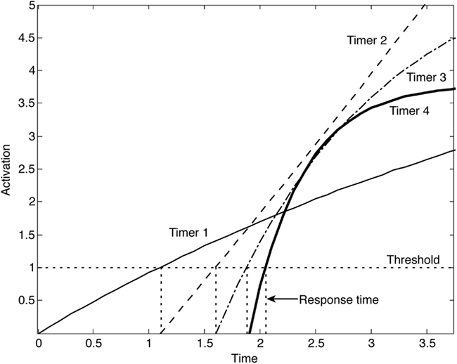
Figure 1. Activation time histories for four sequentially triggered interval timers, based on imperfectly balanced integrators (for each timer, k is selected from a normal distribution with mean and SD of 0.1). Here τ1 = 1, τ2= 0.5, τ3 = 0.25, τ4 = 0.125. Below threshold, these activations are approximately linear.
The mystery of robust temporal integration may therefore reduce to distributing integration tasks to a suite of mechanisms with a range of intrinsic time constants. Each integrator in this scheme triggers the next integrator (with a smaller τ) to ramp up over a time span most appropriate for it. Within each time span, deviations from perfect integration thus remain within tolerable levels. Robust integration may therefore require less in the way of special mechanisms than is sometimes thought, suggesting that theories of timing and perceptual decision-making based on perfect integration are not neurally implausible a priori.
Acknowledgments
This work was supported by the National Institute of Mental Health (P50 MH062196, Cognitive and Neural Mechanisms of Conflict and Control, Silvio M. Conte Center), by the Air Force Research Laboratory (FA9550-07-1-0537), and by an FP7 Marie Curie IRG 277015 to Fuat Balci.
References
Gibbon, J. (1977). Scalar expectancy theory and Weber’s law in animal timing. Psychol. Rev. 84, 279–325.
Luce, R. D. (1986). Response Times: Their Role in Inferring Elementary Mental Organization. New York: Oxford University Press.
Ratcliff, R., and Rouder, J. N. (1998). Modeling response times for two-choice decisions. Psychol. Sci. 9, 347–356.
Rivest, F., and Bengio, Y. (2011). Adaptive drift-diffusion process to learn time intervals. arXiv, 1103.2382v1.
Seung, H. S. (1996). How the brain keeps the eyes still. Proc. Natl. Acad. Sci. U.S.A. 93, 13339–13344.
Shadlen, M. N., and Newsome, W. T. (1994). Noise, neural codes and cortical organization. Curr. Opin. Neurobiol. 4, 569–579.
Citation: Simen P, Balci F, deSouza L, Cohen JD and Holmes P (2011) Interval timing by long-range temporal integration. Front. Integr. Neurosci. 5:28. doi: 10.3389/fnint.2011.00028
Received: 01 June 2011; Accepted: 13 June 2011; Published online: 01 July 2011.
Copyright: © 2011 Simen, Balci, deSouza, Cohen and Holmes. This is an open-access article subject to a non-exclusive license between the authors and Frontiers Media SA, which permits use, distribution and reproduction in other forums, provided the original authors and source are credited and other Frontiers conditions are complied with.
*Correspondence:cHNpbWVuQG1hdGgucHJpbmNldG9uLmVkdQ==