Study on a simulation method for photovoltaic power output series based on the headroom model

Existing photovoltaic (PV) output simulation methods often rely on artificial neural networks for short-term forecasting, and there has been a struggle to capture long-term patterns and stochastic fluctuations when using Markov Chain Monte Carlo techniques. To address these limitations, this paper proposes an improved headroom model-based approach that enhances traditional methods in three key aspects. First, unlike traditional headroom models that ignore temporal dependencies in output fluctuations, the approach integrates probabilistic distributions with soft sequential constraints to preserve time-dependent patterns. Second, whereas previous studies often overlooked seasonal weather variations, here PV output curves are classified into representative weather types and seasonally adaptive Markov chains are constructed to model radiation dynamics and transition probabilities. Third, to address the oversimplification of sunrise and sunset transitions, the method introduces a specialized statistical correction tailored to these critical periods. The method accurately models PV output patterns and fluctuations, demonstrating < 1% deviation in annual duration (4,121 h) and utilization (1,297 h), with a 7.80%−14.59% lower root mean square error and 10.27%−14.07% reduced mean absolute error vs. conventional methods. It efficiently generates realistic long-term sequences from limited data, enhancing the accuracy and efficiency of PV power sequence simulation.

1 Introduction

Energy is the foundation of sustainable economic and social development and is an indispensable power guarantee for human production and life (Liu C. C. et al., 2022). As an important part of renewable energy (Li P. D. et al., 2022), photovoltaic (PV) power generation in China has been developing rapidly in recent years, effectively alleviating both the energy crisis and environmental pressures (Liu J. et al., 2023). However, the output power of PV power generation systems is easily affected by environmental factors such as irradiation and temperature, and it exhibits significant randomness and uncertainty compared to traditional power sources (Zhou et al., 2023). These issues pose a huge challenge to the safety and reliability of power system operations. Simulating the output curve of PVs is important for the optimal design of PV power plants, grid configuration planning, and the formulation of new energy policies (Lee et al., 2021).

PV output curve modeling methods can be divided into two main categories based on the modeling object (Dong et al., 2023). The first category is the modeling method based on solar irradiation intensity, also known as the indirect method, which generally uses physical methods, statistical methods, or learning methods to establish a model of solar irradiation, and then the appropriate photovoltaic cell model for photovoltaic conversion to obtain the photovoltaic output model (Wang et al., 2022). The relevant literature is based on this idea, which first establishes the optimal probability model for radiation intensity, and then obtains the PV output according to the PV conversion rate (Benchrifa et al., 2023; Mishra et al., 2023). This method can clearly reflect the physical meaning and better reflect the regular changes, but it requires a large amount of detailed meteorological data and it is difficult to accurately fit the PV conversion relationship of different PV cell inversion processes, making it difficult to put into practical use most of the time (Liu, 2022).

The second category is the power-based modeling method, also known as the direct method, which uses algorithms to find the mathematical relationship between measured PV historical output data, and directly simulates new PV output sequences based on that historical data (Zhi et al., 2023). The main algorithms used in the current research approaches are artificial neural networks (ANNs), deep learning models, and Monte Carlo Markov Chains. Kallio and Siroux (2023) developed prediction models using multiple linear regression and ANNs, demonstrating that the ANN model trained on individual PV output data achieved the highest accuracy. While ANNs excel at capturing non-linear relationships in short-term PV forecasting, their performance strongly depends on the quality and quantity of training data. Additionally, ANN models are prone to overfitting when applied to medium- and long-term simulations, limiting their generalization capability. Meng et al. (2021) adopted a deep learning-based approach to identify highly correlated meteorological variables under different weather conditions. This method improved the mapping between meteorological factors and power output while reducing computational training time. However, deep learning models require extensive hyperparameter tuning and large datasets. Yang et al. (2023) proposed a hybrid PV power prediction method combining similar days selection, gray-Markov models, and AdaBoost. Their approach used Markov chains to correct gray-Markov prediction errors and integrated them via the BP-AdaBoost algorithm. While this method improved prediction robustness by combining multiple techniques, the gray-Markov model itself struggles with highly stochastic PV output fluctuations, particularly in long-term simulations where weather variability introduces significant uncertainty.

The modeling of PV output time based on the headroom model combines the above two methods, better simulating the generation of sequences of any length with a small amount of data, and so is suitable for the medium- and long-term simulation of PV output sequences. However, current research on the simulation of PV output sequences based on the headroom model often ignores the time-series characteristics of fluctuations in historical sequences. At the same time, it is difficult to reflect the fluctuating characteristics of PV output with seasonal and weather changes. Therefore, in this paper we choose to improve the traditional simulation method based on the headroom model. Li (2015) estimated the maximum value of solar radiation under ideal conditions using the headroom model and modeled the deterministic and uncertain components of the PV output separately to reflect regular changes and accurately simulate the PV output time series. Therefore, in this paper we will demonstrate the effectiveness of the proposed method by comparing it with the method in Li (2015).

Using the traditional simulation method based on the headroom model, we propose a new PV output simulation method. First, the relative PV output is decomposed into a base value and an offset value, and probability models are established for different weather types. Then, the weather transfer probability is calculated separately for each season, and a weather Markov chain is generated at random. Finally, the base value and offset value are sampled using a method that takes into account the volatility of the time series. After correcting the sunrise and sunset times, the PV output sequence is restored according to the headroom model. The simulation is based on data from a specific location in Guangdong Province in 2023. The results show that compared with the traditional method used in Li (2015), the simulation sequence generated by the method in this paper more effectively retains the probability distribution and autocorrelation of the historical PV output sequence, while also inheriting the seasonality of the historical sequence. It can provide a basis for the dispatching plan and operation mode arrangement of the power grid.

2 Analysis of PV output based on the headroom model

The active output of a PV system is affected by light, including both deterministic (e.g., periodic variations in solar radiation) and stochastic factors (e.g., air quality, cloud cover). Therefore, the PV output can be divided into deterministic and stochastic parts; the deterministic part can be simulated by a headroom model, while the stochastic part needs to be described by other models to more accurately reflect the output variations.

2.1 Principles of the headroom model

2.1.1 Solar phototransport process

Energy on Earth comes primarily from the sun—it travels through the atmosphere to the surface in the form of radiation, which is categorized into direct and diffuse radiation (Xu et al., 2024). For any point on Earth, the intensity of radiation directly from the sun onto Earth's atmosphere can be calculated using Equation 1 (Erol and Filik, 2022):

$\begin{array}{ll}{I}_{\text{0}}=S_{\text{0}}\left[1+0.033cos\left(\frac{2\pi (N+10)}{365}\right)\right]& (1)\end{array}$

where I₀ is the intensity of solar radiation perpendicular to the atmosphere, S₀ is the solar constant (which represents the total amount of solar radiation received per unit area perpendicular to the rays of light entering Earth's atmosphere, and takes the value of 1,367 W/m²), and N is the date sequence number of the year, starting from 1 January.

2.1.2 Solar position model

The solar incidence angle, i.e., the angle between the solar incidence ray and the normal to the inclined plane, can be calculated using Equations 2–5, assuming that the attenuating effect of the atmosphere on the intensity of solar irradiation is not taken into account (Masevhe and Maluta, 2022):

$\begin{array}{ll}sin\alpha =sin\delta sin\varphi +sin\delta sin\varphi cos\omega & (2)\end{array}$

$\begin{array}{ll}\omega =(12-t)15^{•}+(120^{•}-\psi )& (3)\end{array}$

$\begin{array}{ll}\delta \approx 2\pi \frac{23.45^{•}}{360^{•}}sin\left(2\pi \frac{284+N}{365}\right)& (4)\end{array}$

$\begin{array}{cc}cos{\theta }_i=cos\beta sin\alpha +sin\beta sin\gamma cos\delta sin& \omega +sin\beta cos\gamma cos\delta \\ (sin\varphi cos\omega -sin\delta )& (5)\end{array}$

where α denotes the solar altitude angle, ω the solar time angle, ϕ the local latitude, δ the declination angle, and β is the tilt angle and γ the azimuth angle of the PV array panels.

2.1.3 Effect of the atmosphere on the intensity of solar radiation

The atmospheric transparency coefficient is the percentage of Earth's atmosphere that allows the passage of solar radiation. Denoting the atmospheric mass by M_hand the atmospheric transparency factor for direct radiation by τ_b, the atmospheric transparency coefficient for direct solar radiation under full sunny conditions can be calculated using Equations 6, 7 (Zhou et al., 2022):

$\begin{array}{ll}{\tau }_{\text{b}}=0.56(e^{-0.56M_{\text{h}}}+e^{-0.096M_{\text{h}}})& (6)\end{array}$

$\begin{array}{ll}{M}_h\text{'}={\left[1229+{\left(614\sin \alpha \right)}^2\right]}^{\frac{1}{2}}-614\sin \alpha & (7)\end{array}$

For higher elevations, we correct for the atmospheric quality of the area using Equation 8:

$\begin{array}{ll}{M}_{\text{h}}\text{'}=M_{\text{h}}\frac{P\left(z\right)}{P_0}=M_{\text{h}}{\left(\frac{288-0.065z}{288}\right)}^{5.256}& (8)\end{array}$

where $M_{\text{h}}\text{'}$ is the corrected atmospheric quality,z is the altitude of the area, and $\frac{P(z)}{P_0}$ is the atmospheric quality correction factor.

The instantaneous direct solar radiation I_b is obtained from Equation 9 (Ding et al., 2024):

$\begin{array}{ll}{I}_{\text{b}}=I_{\text{0}}{\tau }_{\text{b}}cos{\theta }_{\text{i}}& (9)\end{array}$

Approximating the atmospheric transparency coefficient of diffuse radiation, τ_d, by assuming a linear relationship between it and direct radiation (Liu et al., 2022) gives us Equation 10:

$\begin{array}{ll}{\tau }_{\text{d}}=0.271-0.274{\tau }_{\text{b}}& (10)\end{array}$

According to Equation 11, the intensity of solar radiation is Ding et al. (2024)

$\begin{array}{ll}{I}_{\text{d}}=\frac{1}{2}sin\alpha \frac{1-{\tau }_{\text{d}}}{1-1.4ln\frac{{\tau }_{\text{d}}}{M_{\text{h}}}}& (11)\end{array}$

where k is a parameter related to atmospheric quality. When the atmospheric quality is poor, k takes a value between 0.6 and 0.7; when the atmospheric quality is normal, k takes a value between 0.7 and 0.8; when the atmospheric quality is better than normal, k takes a value between 0.8 and 0.9.

In summary, the total solar radiation intensity at a location on Earth at time t can be calculated from Equation 12 without considering random factors (Sheng et al., 2022):

$\begin{array}{ll}{I}_{\text{t}}=I_{\text{b}}+I_{\text{d}}& (12)\end{array}$

The intensity of solar radiation received under headroom conditions on the PV panels at any location and moment on Earth can be calculated using (Equation 12).

From this analysis, it can be seen that the level of PV output is affected by both deterministic and stochastic factors. Therefore, to improve the accuracy of the PV output model, it is divided into two parts (Equation 13):

$\begin{array}{ll}P(i,t)=P_{\text{DCI}}(i,t)*P_{\text{N}}(i,t)& (13)\end{array}$

where P_N(i, t), P(i, t), and P_DCI(i, t) are the PV relative output, PV actual output, and headroom output, respectively, at moment t of day i. The headroom output is the PV output generated by the intensity of solar radiation in the absence of any shading in the headroom condition, which is an analytical function of time, geographic location, and the tilt angle of the PV panels (Wang et al., 2020). The specific solution process can be referred to in the literature (Li, 2015), and will not be repeated here.

The relative output is decomposed into a power baseline value P_S(i) and a power offset value ΔP_N(i, t) through Equations 14, 15:

$\begin{array}{ll}{P}_{\text{N}}(i,t)=P_{\text{S}}(i)+\Delta P_{\text{N}}(i,t)& (14)\end{array}$

$\begin{array}{ll}{P}_{\text{S}}(i)=\frac{1}{n}{\displaystyle \sum _{i=1}^n}{P}_{\text{N}}(i,t)& (15)\end{array}$

where the baseline value corresponds to the average value of daily output, reflecting the intensity of solar radiation throughout the day, and the offset value is the output minus the average value at each moment, reflecting the fluctuation of solar radiation. In what follows, the uncertainty part of the PV is modeled based on the reference value and offset value respectively.

3 Method for PV output simulation

The specific flow of PV simulation is shown in Figure 1, which summarizes the following steps:

Figure 1

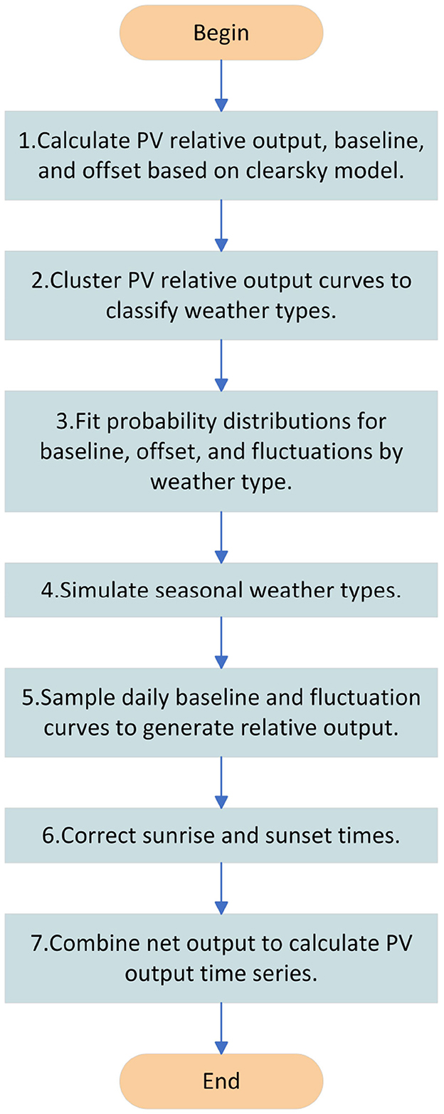
Figure 1. Flowchart showing the PV output simulation procedure.

Step 1. Calculate the PV relative output, the baseline value, and the offset value based on the headroom model. The principle of calculating the PV relative output based on the headroom model and splitting it into the base value and offset value was specifically introduced in Section 1.

Step 2. Cluster PV relative output curves to classify weather types. By adopting a self-organizing map (SOM; see Section 3.1.1), the PV output curve is divided according to the clustering result, and each curve corresponds to the weather type.

Step 3. Fit probability distributions for baseline, offset, and fluctuations by weather type. A kernel density estimation method is used to fit the probability distribution of the normal output moment benchmark value, offset value, and fluctuation value for each type of weather. The statistics for each time period relative to the previous time period relative power difference, are called the fluctuation value.

Step 4. Simulate weather types by season. The weather clustering results in seasons, respectively, the number of weather types and transfer probability, generate a weather Markov chain, which randomly generates the weather type of each day.

Step 5. Sample daily baseline and fluctuation curves to generate relative output. According to the weather type, sample simulation each day's benchmark value and fluctuation coefficient curve to obtain the PV relative output curve.

Step 6. Correct sunrise and sunset times. Consider 1 h after the start of daily PV output and 1 h before the end of output as the sunrise and sunset time of each day, and correct the relative output of this time.

Step 7. Combine the net outputs to calculate the PV output time series. The PV relative output obtained from the simulation is multiplied by the headroom output to obtain the actual PV output.

3.1 Weather type classification and weather type simulation

3.1.1 Comparison of security efficiency

Weather factors affect the amount of solar radiation received by the PV power plant, which in turn affects its output (Hui et al., 2022). The relative PV output curves are significantly different for different weather factors (Wang et al., 2024). Since the fluctuation characteristics of the PV output are only related to the thickness of cloud cover, it is not necessary to classify many weather types for PV output time-series modeling, and it is only necessary to classify the generalized weather types obtained through the clustering analysis of PV output curves.

An SOM is a kind of unsupervised learning network, the complex can realize the dimensional mapping from the input space (n-dimensional) to the output plane (2-dimensional), and the mapping has topological feature preservation properties (Liu S. Q. et al., 2023). In this paper, we adopt an SOM method to select four feature quantities of one day's output data to form feature vectors instead of the relative output curve vectors of photovoltaic power plants for clustering analysis, and divide the photovoltaic output curves according to the clustering results. Each class of curves corresponds to a different type of weather. The four selected eigenquantities are the base value, standard deviation, first-order difference absolute mean, and first-order difference absolute maximum, and they are calculated as follows:

• Baseline value, d₁. This index reflects the level of output throughout the day, e.g., high on sunny days and low on rainy days, and can be calculated from Equation 16:

$\begin{array}{ll}{d}_1=\frac{1}{n}{\displaystyle \sum _{i=1}^n}{P}_{\text{N}}(i)& (16)\end{array}$

where P_N(i) represents the relative PV output at the ith moment of the day.

• Standard deviation, d₂. This index reflects the level of fluctuation throughout the day, e.g., low on sunny and rainy days and high on cloudy days, and can be calculated from Equation 17:

$\begin{array}{ll}{d}_2=\sqrt{\frac{1}{n}{\displaystyle \sum _{i=1}^n}{(P_{\text{N}}(i)-d_1)}^2}& (17)\end{array}$

• Mean of the absolute value of fluctuation value, d₃. This index reflects the level of temporal fluctuations, e.g., high on cloudy days, and can be calculated from Equation 18:

$\begin{array}{ll}\begin{array}{c}{v}_0=|P_{\text{N}}(i+1)-P_{\text{N}}(i)|\\ d_3=\frac{1}{n-1}{\displaystyle \sum _{i=1}^{n-1}}{v}_0\end{array}& (18)\end{array}$

where v₀ is the relative output difference of each time period relative to the previous time period; that is, the first-order difference of the offset value, which is called the fluctuation value.

• Maximum of the absolute value of fluctuation value, d₄. This index reflects the intensity of fluctuations, e.g., high on cloudy or sudden weather, and can be calculated from Equation 19:

$\begin{array}{ll}{d}_4=max{v}_0& (19)\end{array}$

To ensure that the weights of the eigenvalues are the same, the input to the neural network needs to be normalized.

3.1.2 Simulation of weather transfer characteristics

After the weather types are obtained from clustering, the sequence of weather types throughout the year needs to be further determined. For any stochastic process, when the state at a certain moment is known, the subsequent states are only related to the state at that moment, but not to the state before that moment; this transfer property that the probability distribution of the next state can only be determined by the current state is known as the Markov property. A Markov chain is the discrete-time stochastic process model with the Markov property for the stochastic process in the state space after the transition from one state to another (Ying and Lin, 2024).

When studying the transfer characteristics of weather, it can be assumed that today's weather state only relates to yesterday, and the simulation of the sequence of weather types throughout the year can be regarded as a Markov stochastic process (Kolios et al., 2023). That is, by using Markov chains to simulate the transition between various types of weather, the clustering of the weather types can be statistically obtained from the historical weather process transfer probability matrix.

According to Section 2.2.1, the daily output profiles have been classified into a number of weather types, Z = 1, 2, …, k, using the SOM method. The transitions between weather types can be represented by a state transfer matrixP_z and a cumulative state transfer matrix Q_z, both of which can be expressed as a k×k square matrix:

$\begin{array}{ll}{P}_z=\left[\begin{array}{cccc}{p}_{11}& p_{12}& \dots & p_{1k}\\ p_{21}& p_{22}& \dots & p_{2k}\\ ⋮& ⋮& \ddots & ⋮\\ p_{k1}& p_{k2}& \dots & p_{kk}\end{array}\right]& (20)\end{array}$

$\begin{array}{ll}{Q}_z=\left[\begin{array}{cccc}{p}_{11}& p_{11}+p_{12}& \dots & {\displaystyle \sum _{i=1}^k}{p}_{1i}\\ p_{21}& p_{21}+p_{22}& \dots & {\displaystyle \sum _{i=1}^k}{p}_{2i}\\ ⋮& ⋮& \ddots & ⋮\\ p_{k1}& p_{k1}+p_{k2}& \dots & {\displaystyle \sum _{i=1}^k}{p}_{ki}\end{array}\right]& (21)\end{array}$

where p_ij = P(Z_n+1 = j|Z_n = i) denotes the conditional probability that today is of type i and tomorrow is of type j. After establishing the state transfer matrix P_z and the cumulative state transfer matrix Q_z based on the historical weather data, a first-order Markov chain Z = {Z₁, Z₂, …, Z_N} can be generated to simulate the transfer characteristics of the weather changes within N days.

The probability distributions of the weather for different seasons are also different. Therefore, it is necessary to count the number of times and the transfer probability of each weather type separately by season, and generate the weather Markov chain to select the transfer matrix for the corresponding season.

3.2 PV output time-series simulation

3.2.1 Distribution fitting based on kernel density estimation (KDE)

The stochastic modeling of PV output requires the probability distribution of statistical PV output characteristics. The general research idea is to first assume that the solar irradiance or other influencing factors obey a certain parameter distribution, and then estimate the parameters of the distribution using historical data. This research method has certain limitations: parameter selection is subjective, and the theoretical basis is not sufficient. Moreover, most of the existing related research focuses on the parameter distribution of a specific influencing factor, and it is difficult to comprehensively reflect the stochasticity. Therefore, the preset parameter distribution cannot be applied.

Therefore, in this paper, we choose to use kernel density estimation (KDE) for parameter fitting, which is a method that does not require any a priori knowledge, instead taking the characteristics of the data distribution completely from the data samples; this method has been applied to load modeling and wind speed modeling (Li M. et al., 2022). Its specific principle is more complicated and has been demonstrated in the literature, so it will not be repeated here (see Hou et al., 2022).

For modeling PV stochasticity, we fit probability distributions to the baseline and offset values of the PV relative output. However, extracting only the offset value of each time period in turn does not enable a reflection of the time-ordered nature of PV series fluctuations. Therefore, it is necessary to count the relative output difference of each time period relative to the previous time period; that is, the fluctuation value v₀.

Bandwidth selection plays a critical role in non-parametric KDE modeling. Excessive bandwidth leads to oversmoothing of the probability density function, obscuring essential structural features, while insufficient bandwidth results in overfitting through the inclusion of spurious local fluctuations. In this study, the optimal bandwidth for each weather type is determined using an established formula (Rao et al., 2023). The impact of bandwidth selection on the simulated PV output sequences will be further examined in Section 4 (Case Study) to validate modeling robustness.

3.2.2 Sampling method considering the time-ordered nature of PV series fluctuations

After completing the extraction of the output characteristics and weather transfer characteristics of the original sequence, the simulation of the PV sequence can be performed. The overall simulation process is shown in Figure 2. The specific steps are as follows.

Figure 2

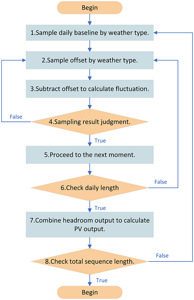
Figure 2. Flowchart showing the PV relative output sequence simulation procedure.

Step 1. Sample daily baseline by weather type. Simple sampling of daily baseline values based on randomly generated weather chains.

Step 2. Sample offset by weather type. Simple sampling of daily offset values based on randomly generated weather chains.

Step 3. Subtract offset to calculate fluctuation. Take the current moment's offset value and subtract it from the value at the previous moment to get a sample of the fluctuation value v₀.

Step 4. Judge sampling result. Denote the probability density distribution function of v₀ as f(v₀). Construct a new probability density function q(v₀), satisfying kq(v₀)>f(v₀), where k is a constant. Sample [0, kq(v₀)] uniformly to get u₀. If u₀<f(v₀), then accept this sampling and go to the next moment. Otherwise reject this sampling and resample the offset value distribution until the sampling is accepted.

Step 5. Proceed to the next moment. Accept this sampling to get the offset value for that moment.

Step 6. Check daily length. If sampling has been completed at all moments of the current day, calculate the relative PV output at all moments of the current day and proceed to the next day. Otherwise return to step 2.

Step 7. Combine headroom output to calculate PV output. Multiply the simulated relative PV output by the headroom output to obtain the actual PV output.

Step 8. Check total sequence length. If all days of the simulation sequence have been generated all day PV relative output, output PV relative output simulation sequence, otherwise return to step 1.

3.2.3 Sunrise and sunset time correction

The periods of 1 h after the start of the daily PV output and 1 h before the end of the output are regarded as the daily sunrise and sunset hours. Compared with the normal power time, the relative power of each weather type is shown to fluctuate around the benchmark value, and the relative power of the sunrise and sunset hours is shown to have an upward or downward trend. Therefore, it is necessary to correct this period of time using separate statistics, as shown in Figure 3. The specific steps are as follows.

Figure 3

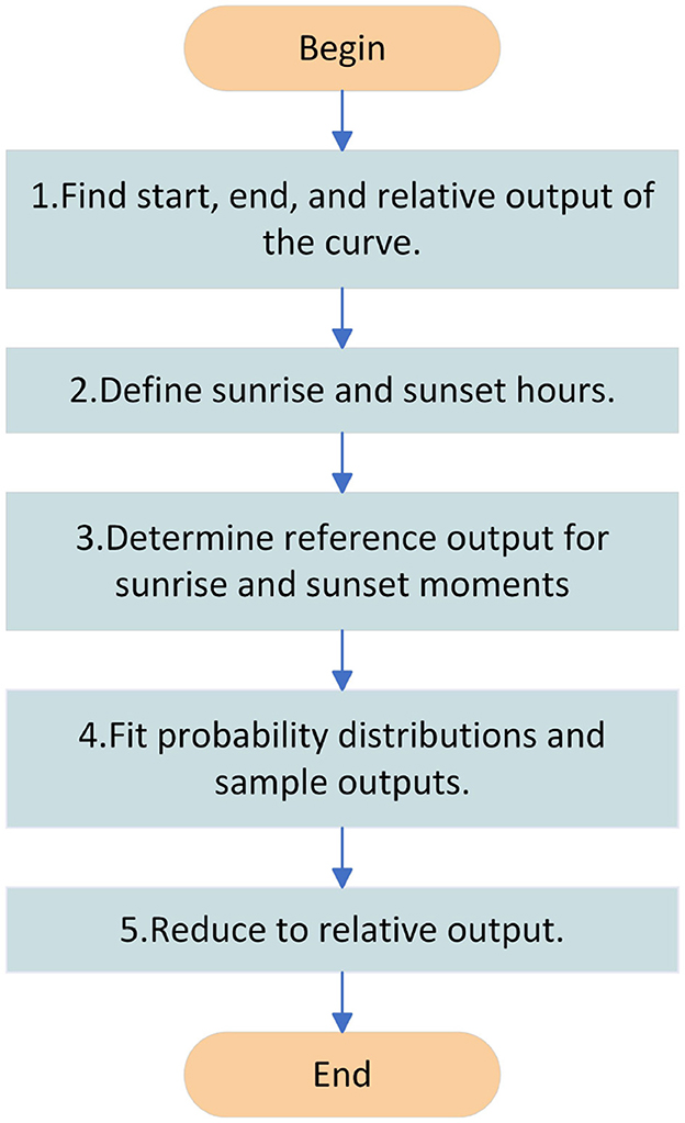
Figure 3. Flowchart showing the sunrise and sunset time correction process.

Step 1. Find the starting moment T_rise, ending moment T_set, and the corresponding relative output values P_Nrise and P_Nset of the relative output curve for each day.

Step 2. Define the sunrise and sunset hours. The five moments after the starting moment are defined as sunrise hours and the five moments after the ending moment are defined as sunset hours.

Step 3. Determine the reference output for each moment of the sunrise hour and each moment of the sunset hour, respectively. The ratio of the relative output to each moment of the sunrise period and the ratio of the relative output to each moment of the sunset period are used as reference outputs.

Step 4. Fitting probability distributions to reference outflows at each moment separately and sampling. Probability distributions were fitted to the reference outflows at each moment separately for the sub-seasons and sampled.

Step 5. Reduction to relative output. Reduction of the reference output obtained by sampling at each moment in time to the relative output.

4 Case study

4.1 Boundary conditions

In this paper, the effectiveness of the proposed method is modeled and verified based on the 2023 output historical data of a PV station in Yangjiang, Guangdong Province. The time resolution of this data is 10 min, which gives 144 pieces of data per day. The power station is located at approximately 21.8°N, 112°E, and the rated capacity is 100 MW. The simulation environment is MATLAB 2022a.

Figure 4 shows the historical data output for the whole year, where the deterministic data and uncertainty of the PV output can be observed. The deterministic data includes the daily characteristics of the daily output, which rises after sunrise, reaching an extreme value at noon, and then declines to zero output at sunset. The deterministic data also includes the regular variations of annual characteristics such as long output time in summer, followed by the second-longest output time in spring and fall, and the shortest output time in winter. Uncertainty includes random variations influenced by weather.

Figure 4

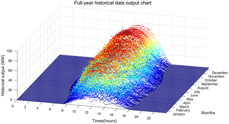
Figure 4. Full-year historical data.

4.2 Analysis of PV relative output

The modeling data are missing the tilt angle and horizontal angle of the photovoltaic array. For this situation, the specific principle of this paper for estimating installation information is that the headroom power is the ideal power, and the parameter is roughly estimated according to whether the power time period is covered, and then it is checked whether the specific daily power curve is enveloped for fine-tuning. Figure 5 shows the specific time periods of the historical annual PV output and the headroom output. As can be seen from the figure, the daily headroom output curve envelopes the historical output curve. Although there is a certain deviation from the actual situation due to the lack of the tilt and horizontal angles of the PV array, it will not have a significant impact on the simulation results because the headroom model is used during the simulation process to transform and invert the actual power and relative power. As long as the actual power can be completely enclosed by the headroom power during the normal power output period, it will have little impact on clustering, statistics, modeling, and sampling during the process.

Figure 5

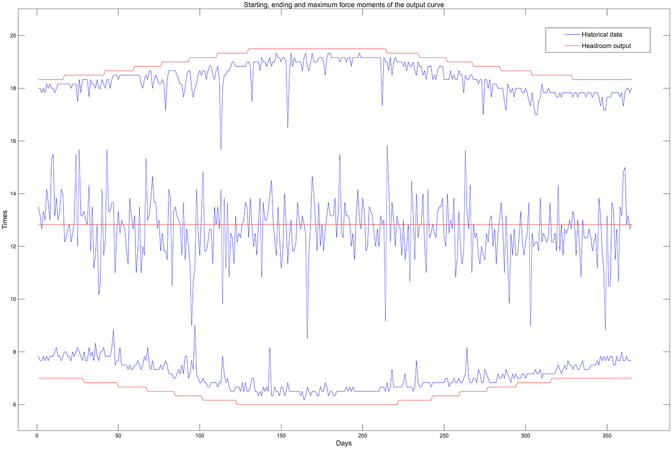
Figure 5. Headroom Output periods for historical and headroom sequences.

Observation of the labeled part of Figure 5 reveals that, unlike the netting sequence, the historical sequence power out time does not show a better symmetry, with the starting moment in January–March significantly later than the netting sequence, and the power out time being delayed as a whole, while in September–December, the sunset moment is earlier than that of the headroom sequence and the power output moment is advanced overall. This phenomenon may be due to the installation of each PV panel tilt angle and the horizontal angle is not the same as the result; if there is a large impact, using multiple sets of parameters to simulate the combination of each PV panel could be considered to obtain the target effect.

After obtaining the headroom model, the relative output of the historical series is calculated and split into the baseline and offset values. The last week of data is selected for display in Figure 6, where it can be seen that the daily curves are quite different, representing different weather types, and so it is necessary to model them separately. Meanwhile, it can be observed that at sunset on the last day, the relative output appears to climb abnormally; the reason and correction method for this are discussed in Section 3.2.3.

Figure 6

Figure 6. Historical and relative output during a one-week period.

4.3 Weather classification

We process the relative output of the historical series of normal hours, calculating the four characteristic values of the daily output curve (baseline value, standard deviation, mean of the absolute value of fluctuation value, and maximum of the absolute value of fluctuation value), and inputting them into the SOM neural network for clustering after normalization. Using the Davies–Bouldin Index (Li and Liu, 2022), it was determined that they could be classified into six classes. These classes are named according to their output characteristics: cloudy, rainy, sudden change, sunny, cloudy A, and cloudy B (cloudy A has a medium average output level but high fluctuation, while cloudy B has a high average output level and medium fluctuation). The typical output curves for each category are shown in Figure 7.

Figure 7

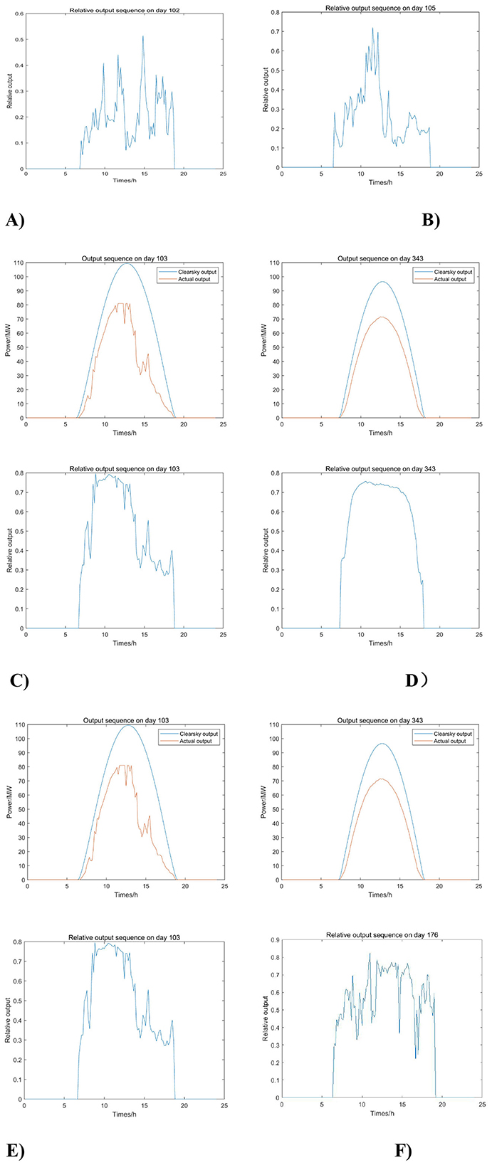
Figure 7. Historical output curves for the six types of weather. (A) Overcast, (B) Rainy, (C) Sudden change, (D) Sunny, (E) Cloudy A, and (F) Cloudy B.

As can be seen in Figure 7, the data among the various types of weather are still scattered, and parameter fitting may be difficult when fitting probability distributions of the output characteristics, so the KDE non-parametric estimation was chosen to rely only on fitting the data characteristics.

4.4 Simulation of weather type

For seasonal weather clustering, the state transfer matrix was generated by counting the number of times each weather type occurred and the respective transfer probability. Figure 8 shows a schematic diagram of the cumulative transfer matrix for the four seasons. The differences in the probability of weather transfer between seasons are quite large. Therefore, it is necessary for us to calculate the probability of weather transfer for each season separately and sampling to generate the weather chain. We then extract the baseline value for each day and the offset value for each moment according to the weather, and judge whether it is acceptable or not. After the extraction is completed, the correction to the output boundary and the sunrise and sunset hours is carried out. The relative output obtained from the correction is multiplied by the headroom output to obtain the simulated output sequence.

Figure 8

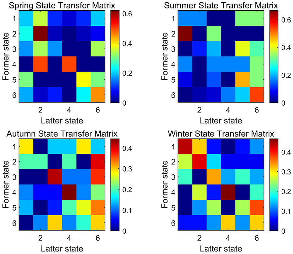
Figure 8. Cumulated transition matrixes for each of the four seasons.

4.5 Simulation results and evaluation

Figure 9 shows the annual simulated power output diagram. Compared with the historical power output in Figure 4, it can be seen that the simulated power output well restores the daily and annual characteristics of the photovoltaic power output. Additionally, the weather changes over a period of time show the seasonality of the historical series well; for example, there are many cloudy and rainy days in winter and spring, and there are many sunny days in summer and autumn.

Figure 9

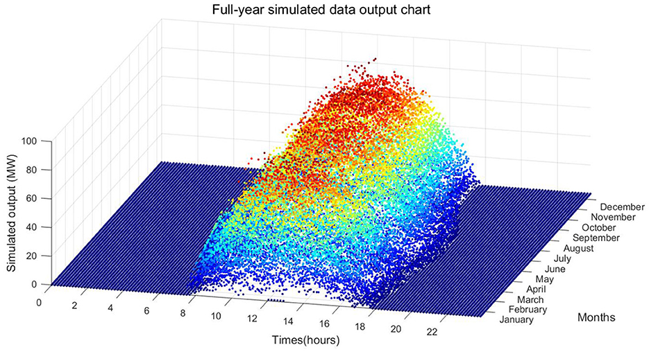
Figure 9. Full-year simulated data.

The overall evaluation of the simulation results, as shown in Table 1, provides further statistical comparison of historical output (Figure 4) and simulated output (Figure 9) for the annual output duration and annual utilization hours. The results show an annual output duration for the historical output of 4160.5 h, and an annual output duration for the simulated output of 4121.3 h (taking into account the Markov chain simulation of weather types and the randomness of sampling the daily baseline values and offset values, the fluctuation range is 4,100–4,190 h). There are 1283.2 annual utilization hours for the historical output and 1296.7 annual utilization hours for the simulated output (the fluctuation range is 1,260–1,340 h). Overall, the error of the key indicators of the two is within an acceptable range, and the annual weather distribution is also relatively consistent, so the simulation results are reliable and valid.

Table 1

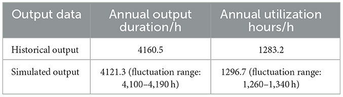
Table 1. Comparison of key indicators for historical and simulated output.

Figure 10 shows the simulated output curves for each type of weather. Observing the generation of specific daily output curves in Figure 10, it can be seen that the output characteristics of the different types weather are well-reflected. Moreover, the sampling method is consistent with the continuity of PV output because the simulated curves do not show frequent and drastic fluctuations within a short period of time due to the consideration of the temporal nature of the fluctuations. In terms of simulation speed, after repeated tests, it takes less than 10 s to generate a PV simulation output sequence with a length of 1 year, and the program runs efficiently.

Figure 10

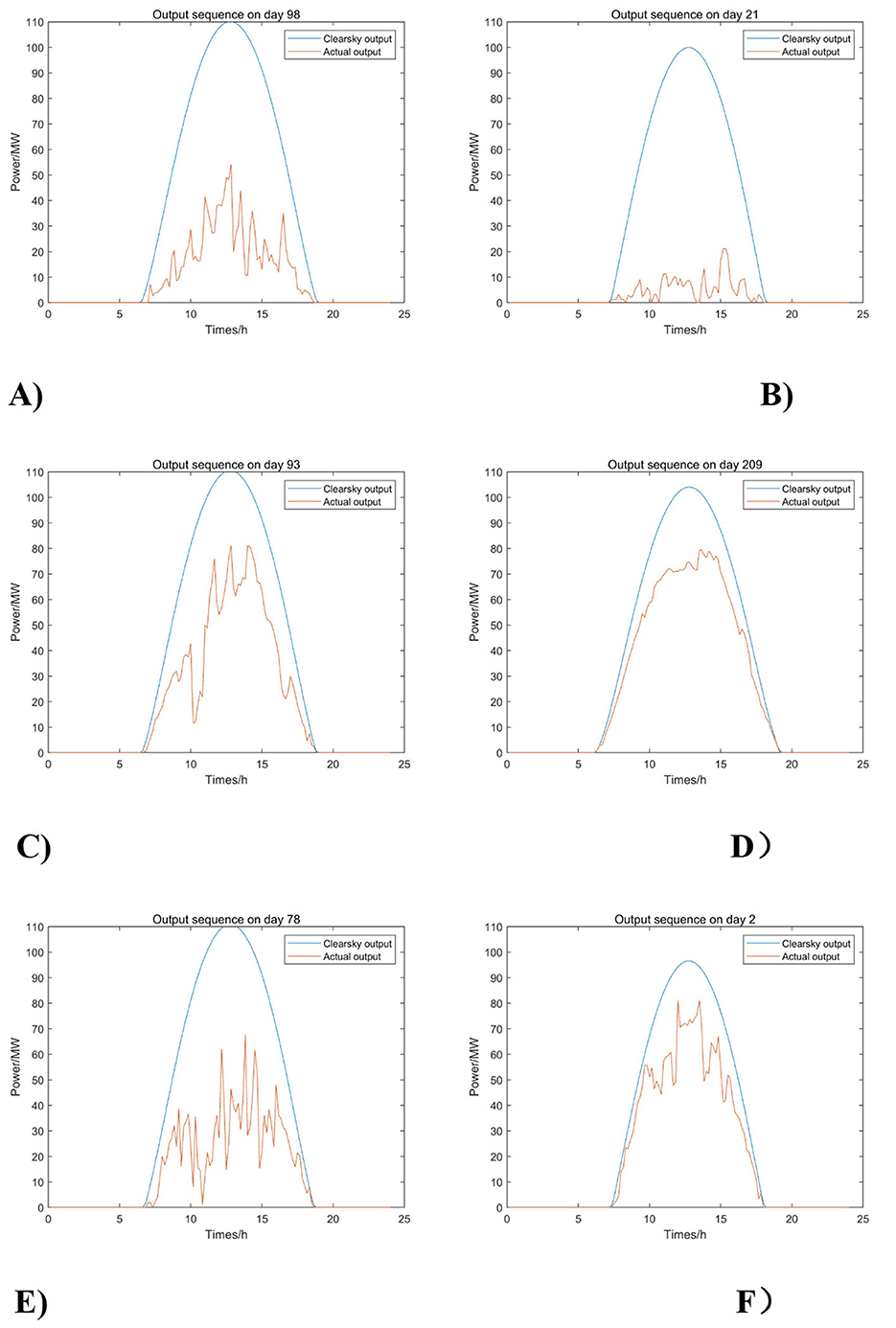
Figure 10. Six weather simulation output curves. (A) Overcast, (B) Rainy, (C) Sudden change, (D) Sunny, (E) Cloudy A, and (F) Cloudy B.

Since the proposed simulation method builds upon the traditional headroom model-based approach (referred to as the original method), its improvements include selective sampling of fluctuation amounts and a correction method for sunrise and sunset times to better restore the characteristics of the historical series. To further validate the effectiveness of the proposed method, the probability density function and autocorrelation function were used to assess whether the simulated results preserve the historical characteristics of the original series. A comparative analysis was conducted of the historical output, the simulated output generated by the original method, and the simulated output generated by the proposed method. The autocorrelation coefficients of the three outputs are presented in Figure 11, while the probability distributions relative to the rated capacity are shown in Figure 12. The results demonstrate that, in terms of both autocorrelation coefficients and probability distribution, the proposed method yields simulation results that align more closely with the historical output than the original method, thereby enhancing the fidelity of historical characteristic restoration.

Figure 11

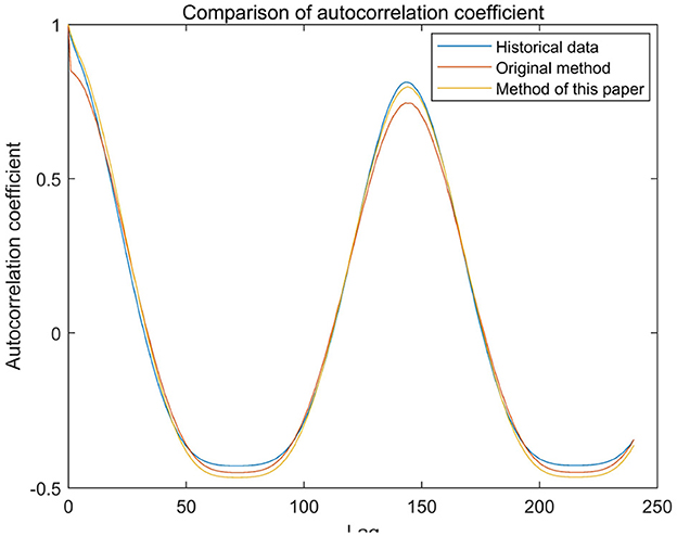
Figure 11. Comparison of the autocorrelation coefficient.

Figure 12

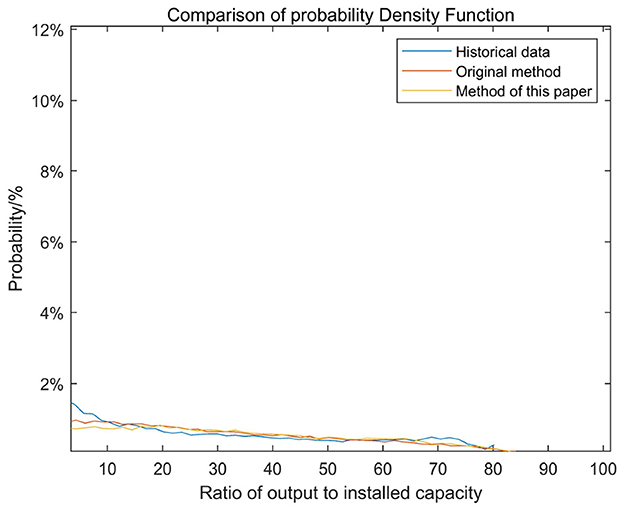
Figure 12. Comparison of the probability density function.

The root mean square error (RMSE), mean absolute error (MAE), and normalized RMSE (NRMSE) were computed for both methods across four distinct seasons. As summarized in Table 2, the proposed method consistently achieves lower RMSE, MAE, and NRMSE values compared to the original method in all seasonal cases. These results quantitatively confirm that the proposed simulation approach more accurately replicates the historical output characteristics than the original method.

Table 2

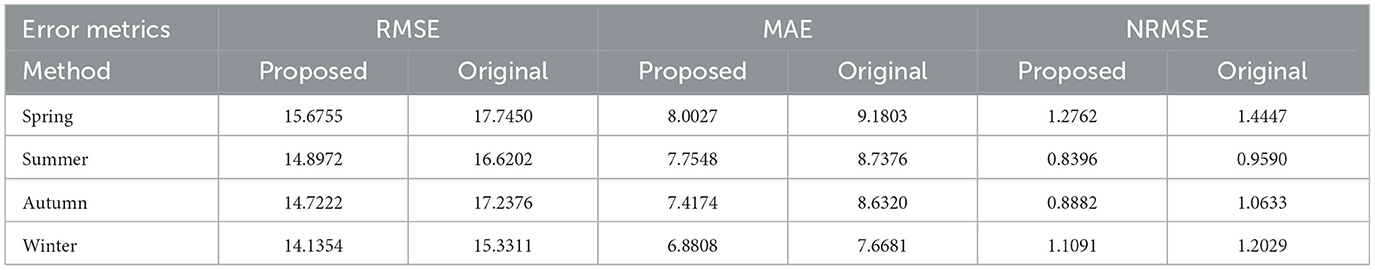
Table 2. Comparison of simulation errors between the proposed and original methods.

4.6 Parameter sensitivity analysis

To comprehensively evaluate the robustness of key parameters in the proposed model, systematic sensitivity analyses were conducted for both the KDE bandwidth selection and the sunrise/sunset correction window length.

For the KDE-based modeling approach, the bandwidth sensitivity was investigated by adjusting the original optimal bandwidth by ±20%, ±15%, ±10%, and ±5%. As illustrated in Figure 13, the resulting RMSE, MAE, and NRMSE metrics for all four seasons exhibit a distinct concave pattern, with minimum values consistently occurring at the original bandwidth setting. This behavior confirms that the bandwidth derived from the established optimal formula represents the most appropriate choice for minimizing simulation errors across different seasonal conditions.

Figure 13

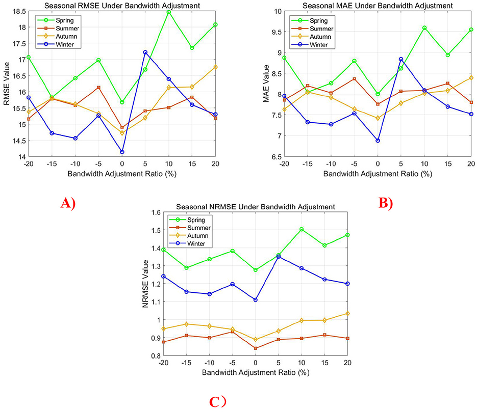
Figure 13. Seasonal error metric variations under bandwidth adjustment. (A) RMSE, (B) MAE, and (C) NRMSE.

Regarding the sunrise/sunset correction, the sensitivity analysis examined window lengths ranging from zero (no correction) to nine time intervals. Figure 14 demonstrates that all three error metrics reach their minimum values when implementing a five-interval correction window, validating the original parameter selection. This optimal window length effectively balances the transitional period characterization while avoiding overcorrection effects.

Figure 14

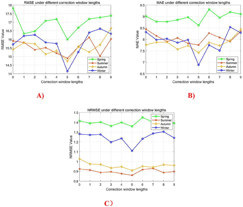
Figure 14. Impact of sunrise/sunset correction window length on simulation accuracy. (A) RMSE, (B) MAE, and (C) NRMSE.

5 Conclusions

This paper proposes a new simulation method for photovoltaic output based on the traditional headroom model. By introducing selective sampling of the fluctuation quantity and improving the correction method at sunrise and sunset, the characteristics of the historical series can be restored with high accuracy. At the same time, when simulating weather types, the probability of weather transfer is statistically analyzed by season to reflect the fluctuating characteristics of PV power output with seasonal and weather changes. Through the simulation of the output of an actual PV power plant, it is verified that the method proposed in this paper can effectively simulate the regular changes and random fluctuations of photovoltaic power generation. We draw the following conclusions.

First, improvements in the sampling method for temporal fluctuations and the correction method for sunrise and sunset times have enhanced the practicality of the model. This paper introduces a selective sampling of the fluctuation amount when sampling the benchmark and offset values of the relative photovoltaic output. Simulation results show that the simulated sequence generated by this sampling method closely matches the historical data in terms of probability distribution and autocorrelation, better reflecting the characteristics of the historical sequence. Validation with operational PV plant data demonstrates superior performance, with a 7.80%−14.59% reduction in RMSE, a 10.27%−14.07% lower MAE, and a 7.80%−16.4% improvement in NRMSE compared to the original method.

Second, the categorization of weather types and the use of Markov chains enhance the flexibility of simulation. Through SOM clustering of the historical data of the PV output, the weather is categorized into multiple types, and Markov chains are used to simulate the transfer probability of different weather, which effectively retains the fluctuating characteristics of the PV output with seasonal and weather changes. The method is able to accurately simulate the regularity and fluctuation of output power under different weather conditions, and is suitable for medium- and long-term simulation.

Last, the case study confirms that the proposed PV simulation method achieves high computational efficiency while accurately replicating actual output characteristics. Key metrics show excellent agreement: annual output duration (4,121 vs. 4,161 historical hours) and utilization hours (1,297 vs. 1,283 historical hours) both demonstrate less than 1% deviation. This precise performance makes the method particularly valuable for grid scheduling, plant design, and policy development applications.

Data availability statement

The raw data supporting the conclusions of this article will be made available by the authors, without undue reservation.

Author contributions

HD: Writing – original draft. YuG: Writing – original draft. LH: Writing – review & editing. YaG: Writing – review & editing. YX: Writing – original draft.

Funding

The author(s) declare that financial support was received for the research and/or publication of this article. This research was funded by the Science and Technology Project of Guangzhou Power Supply Bureau, Guangdong Power Grid Co., Ltd, (GDKJXM20222293 and 030100KK52222015).

Conflict of interest

HD, YuG, LH, and YaG were employed by Guangdong Power Grid Co., Ltd.

The remaining authors declare that the research was conducted in the absence of any commercial or financial relationships that could be construed as a potential conflict of interest.

Generative AI statement

The author(s) declare that no Gen AI was used in the creation of this manuscript.

Any alternative text (alt text) provided alongside figures in this article has been generated by Frontiers with the support of artificial intelligence and reasonable efforts have been made to ensure accuracy, including review by the authors wherever possible. If you identify any issues, please contact us.

Publisher's note

All claims expressed in this article are solely those of the authors and do not necessarily represent those of their affiliated organizations, or those of the publisher, the editors and the reviewers. Any product that may be evaluated in this article, or claim that may be made by its manufacturer, is not guaranteed or endorsed by the publisher.

References

Benchrifa, M., Mabrouki, J., and Tadili, R. (2023). Estimation of Global Irradiation on Horizontal Plane Using Artificial Neural Network. Cham: Springer International Publishing. doi: 10.1007/978-3-031-26254-8_56

Crossref Full Text | Google Scholar

Ding, X., Zhang, S., and Jin, C. (2024). Construction and application of a model for solar radiation in clear skies in complex terrain areas. Acta Energiae Solaris Sin. 45, 569–577. doi: 10.19912/j.0254-0096.tynxb.2022-1961

Crossref Full Text | Google Scholar

Dong, C., Wang, Z., Bai, J., Jiang, J., Wang, B., Liu, G., et al. (2023). Review of ultra-short-term forecasting methods for photovoltaic power generation. High Voltage Eng. 49, 2938–2951. doi: 10.13336/j.1003-6520.hve.20220974

Crossref Full Text | Google Scholar

Erol, Ö., and Filik, Ü. (2022). Improvement and evaluation of daily global solar radiation decomposition models using meteorological parameters: a case study for Turkey. Int. J. Green Energy 19, 1633–1648. doi: 10.1080/15435075.2021.2018592

Crossref Full Text | Google Scholar

Hou, W., Hou, L., Zhao, S., and Liu, W. (2022). A hybrid data-driven robust optimization approach for unit commitment considering volatile wind power. Electric Power Syst. Res. 205:107758. doi: 10.1016/j.epsr.2021.107758

Crossref Full Text | Google Scholar

Hui, L., Ren, Z. Y., Yan, X., Li, W. Y., and Bo, H. (2022). A multi-data driven hybrid learning method for weekly photovoltaic power scenario forecast. IEEE Trans. Sust. Energy 13, 91–100. doi: 10.1109/TSTE.2021.3104656

Crossref Full Text | Google Scholar

Kallio, S., and Siroux, M. (2023). Photovoltaic power prediction for solar micro-grid optimal control. Energy Rep. 9, 594–601. doi: 10.1016/j.egyr.2022.11.081

Crossref Full Text | Google Scholar

Kolios, A., Richmond, M., Koukoura, S., and Yeter, B. (2023). Effect of weather forecast uncertainty on offshore wind farm availability assessment. Ocean Eng. 285:115265. doi: 10.1016/j.oceaneng.2023.115265

Crossref Full Text | Google Scholar

Lee, D., Jeong, J., and Choi, G. (2021). Short term prediction of PV power output generation using hierarchical probabilistic model. Energies 14:2822. doi: 10.3390/en14102822

Crossref Full Text | Google Scholar

Li, C. (2015). Study on the Modeling Method of New Energy Power Time Series Based on Fluctuation Characteristies (Master).

Google Scholar

Li, J., and Liu, Q. B. (2022). Forecasting of short-term photovoltaic power generation using combined interval type-2 Takagi-Sugeno-Kang fuzzy systems. Int. J. Electr. Power Energy Syst. 140:108002. doi: 10.1016/j.ijepes.2022.108002

Crossref Full Text | Google Scholar

Li, M., Yang, M., Yu, Y., and Lee, J. W. (2022). A wind speed correction method based on modified hidden markov model for enhancing wind power forecast. IEEE Trans. Industry Applic. 58, 656–666. doi: 10.1109/TIA.2021.3127145

Crossref Full Text | Google Scholar

Li, P. D., Gao, X. Q., Li, Z. C., and Zhou, Y. X. (2022). Effect of the temperature difference between land and lake on photovoltaic power generation. Renew. Energy 185, 86–95. doi: 10.1016/j.renene.2021.12.011

Crossref Full Text | Google Scholar

Liu, C. C., Li, M., Yu, Y. J., Wu, Z. Y., Gong, H., Cheng, F., et al. (2022). A review of multitemporal and multispatial scales photovoltaic forecasting methods. IEEE Access 10, 35073–35093. doi: 10.1109/ACCESS.2022.3162206

Crossref Full Text | Google Scholar

Liu, J., Lin, S., Liang, W., Wang, Q., and Liu, M. (2023). Short-term probabilistic forecast for power output of photovoltaic station based on high order Markov chain and gaussian mixture model. Power Syst. Technol. 47, 266–275. doi: 10.00-3673/(2023)01-0266-09

Crossref Full Text | Google Scholar

Liu, S. Q., Zhou, X. Z., Li, B., He, X., Zhang, Y. X., Fu, Y., et al. (2023). Improving short-term streamflow forecasting by flow mode clustering. Stochastic Environ. Res. Risk Assess. 37, 1799–1819. doi: 10.1007/s00477-022-02367-z

Crossref Full Text | Google Scholar

Liu, X., Zhang, H., Yan, H., and Luo, J. (2022). Research on the estimation of solar radiation on clear days in complex regional terrain. Acta Energiae Solaris Sin. 43, 174–180. doi: 10.19912/j.0254-0096.tynxb.2021-0127

Crossref Full Text | Google Scholar

Liu, Y. Y. (2022). Short-term prediction method of solar photovoltaic power generation based on machine learning in smart grid. Math. Probl. Eng. doi: 10.1155/2022/8478790

Crossref Full Text | Google Scholar

Masevhe, L., and Maluta, E. N. (2022). Assessment of photovoltaic power output using the estimated global solar radiation at Vuwani Science Resources Centre. Cogent Eng. 9:2105031. doi: 10.1080/23311916.2022.2105031

Crossref Full Text | Google Scholar

Meng, A., Xu, X., Chen, J., Wang, C., Zhou, T., Yin, H., et al. (2021). Ultra short term photovoltaic power prediction based on reinforcement learning and combined deep learning model. Power Syst. Technol. 45, 4721–4728. doi: 10.13335/j.1000-3673.pst.2021.0319

Crossref Full Text | Google Scholar

Mishra, D. P., Jena, S., Senapati, R., Panigrahi, A., and Salkuti, R. S. (2023). Global solar radiation forecast using an ensemble learning approach. Int. J. Power Electr. Drive Syst.S) 14, 496–505. doi: 10.11591/ijpeds.v14.i1.pp496-505

Crossref Full Text | Google Scholar

Rao, Z., Wang, K., Tan, J., Li, J., Yang, Z., Meng, W., et al. (2023). Nonparametric kernel density estimation and analysis of Guangdong offshore wind power output based on optimal bandwidth. Acta Energiaesolaris Sin. 44, 274–282. doi: 10.19912/j.0254-0096.tynxb.2022-1325

Crossref Full Text | Google Scholar

Sheng, X. W., Shi, T., Zheng, W. Q., and Lou, P. (2022). Time-varying non-uniform temperature distributions in concrete box girders caused by solar radiation in various regions in China. Adv. Mech. Eng. 14:6458. doi: 10.1177/16878140221076458

Crossref Full Text | Google Scholar

Wang, J., Huang, Y., Li, C., Xiang, K., and Lin, Y. (2020). Time series modeling method for multi-photovoltaic power stations considering spatial correlation and weather type classification. Power Syst. Technol. 44, 1376–1384. doi: 10.13335/j.1000-3673.pst.2019.0729

Crossref Full Text | Google Scholar

Wang, X. Y., Sun, Y. L., Luo, D., and Peng, Q. J. (2022). Comparative study of machine learning approaches for predicting short-term photovoltaic power output based on weather type classification. Energy 240:122733. doi: 10.1016/j.energy.2021.122733

Crossref Full Text | Google Scholar

Wang, Y. G., Yao, Y. L., Zou, Q. Y., Zhao, K. X., and Hao, Y. (2024). Forecasting a short-term photovoltaic power model based on improved snake optimization, convolutional neural network, and bidirectional long short-term memory network. Sensors 24:3897. doi: 10.3390/s24123897

PubMed Abstract | Crossref Full Text | Google Scholar

Xu, L. T., Ding, P., Zhang, Y., Huang, Y. J., Li, J. M., Ma, H. R., et al. (2024). Sensitivity analysis of the shading effects from obstructions at different positions on solar photovoltaic panels. Energy 290:130229. doi: 10.1016/j.energy.2023.130229

Crossref Full Text | Google Scholar

Yang, X., Wang, S., Peng, Y., Chen, J., and Meng, L. (2023). Short-term photovoltaic power prediction with similar-day integrated by BP-AdaBoost based on the Grey-Markov model. Electric Power Syst. Res. 215:108966. doi: 10.1016/j.epsr.2022.108966

Crossref Full Text | Google Scholar

Ying, H., and Lin, F. (2024). Discrete-time finite fuzzy markov chains realized through supervised learning stochastic fuzzy discrete event systems. IEEE Trans. Fuzzy Syst. 32, 6088–6100. doi: 10.1109/TFUZZ.2024.3440184

Crossref Full Text | Google Scholar

Zhi, Y., Sun, T., and Yang, X. (2023). A physical model with meteorological forecasting for hourly rooftop photovoltaic power prediction. J. Build. Eng. 75:106997. doi: 10.1016/j.jobe.2023.106997

Crossref Full Text | Google Scholar

Zhou, X., Pang, C. X., Zeng, X. H., Jiang, L. H., and Chen, B. Y. (2023). A short-term power prediction method based on temporal convolutional network in virtual power plant photovoltaic system. IEEE Trans. Instrum. Measur. 72:3301904. doi: 10.1109/TIM.2023.3301904

Crossref Full Text | Google Scholar

Zhou, Y., Fu, X., Yang, F., and Wang, Y. (2022). Static security analysis of park-level agricultural energy internet considering spatial coupling. Power Syst. Technol. 46, 995–1004. doi: 10.003673/(2022)03-0995-10

Crossref Full Text | Google Scholar