Contrast Agent Quantification by Using Spatial Information in Dynamic Contrast Enhanced MRI

1 Introduction

MRI contrast agents (CAs) are used to improve the visibility of internal brain structures (Rinck, 2019). With dynamic contrast-enhanced MRI (DCE-MRI), the uptake and washout of an exogenous contrast agent can be monitored in certain tissues, e.g. tumors, vessels and white matter. By analysing the dynamics of the CA concentration using pharmacokinetics models (Sourbron and Buckley, 2013), it is possible to estimate physiology parameters such as blood flow, vessel density, capillary endothelial permeability, and extravascular extracellular space volume. These parameters are useful for characterising e.g. tumor angiogenesis (Verma et al., 2012), performing target delineation and evaluating treatment response in radiotherapy (Cao, 2011).

A crucial step for successful parameter estimation is accurate determination of the CA concentration. This is difficult since MR-signals have a complicated relationship with the CA concentration through the effect of the CA on the tissue relaxation time constants. Most commonly, CA concentration is estimated using the magnitude of the MRI images (Sourbron and Buckley, 2011), which is referred to as magnitude estimated CA in this paper. However, the accuracy of this method can be hampered by for instance issues like flip angle inhomogeneity (Cheng, 2007).

In addition to the magnitude information, MRI images also contain phase information and the phase is influenced by the CA concentration as well. This has been exploited for accurate blood CA estimates and Brynolfsson et al. (2014) combined the magnitude estimated CA and phase shift data to improve CA estimation in all types of tissue. In Brynolfsson et al. (2014), a maximum likelihood estimator (MLE) was used to find the most likely CA concentration given noisy and biased magnitude images and noisy phase images with the assumption that voxels are independent of each other.

In this work, we relax the restrictions in Brynolfsson et al. (2014) by assuming that voxels that are spatially close to each other are not independent. The main contribution of this work is that we utilised the spatial dependence information among voxels to improve the accuracy of CA concentration estimation. For this purpose, spatial statistical modelling approaches, in particular Bayesian hierarchical models (BHMs), are used together with phase shift data and magnitude estimated CA. Furthermore, with improved CA concentration estimation, we are able to increase the estimation accuracy of related physiology parameters and bring potential benefits to patients in terms of precision medicine in tumor treatment. At current stage, we limit our evaluations to simulation data. The DCE-MRI simulation is based on an anatomical model from BrainWeb (Aubert-Broche et al., 2006), where the tissue-specific true CA concentration in voxels is calculated using the modified Kety model (Tofts, 1997). Afterwards, the magnitude estimated CA and phase shift data are simulated through the models 1) and 2) in the next section, with tissue-specific bias and noise. See Brynolfsson et al., 2014 for the simulation details.

The structure of the paper is organized as follows. The models with and without spatial information will be introduced in Section 2. In Section 3, the methods used in this work will be specified. Results will be presented in Section 4. The paper will be closed with conclusion and discussion.

2 Theory

2.1 Magnitude and Phase Models

This work uses the model developed by Brynolfsson et al. (2014) as its starting point. Briefly, the model assumes that a measurement of the CA concentration c = (c₁, … , c_N), where N is the number of voxels in the image, can be obtained using magnitude estimated CA data ${\mathbf{c}}_m=(c_1^m,\dots ,c_N^m)$. In addition to that, the measurement can be also deduced using phase shift data Δφ = (Δφ₁, … , Δφ_N). The statistical model connecting the underlying CA concentration c and the measured data, i.e. magnitude estimated CA and phase shift, has the form

${\mathbf{c}}_m=D_{\mathit{\xi }}\mathbf{c}+{\mathit{\epsilon }}_m(1)$

$\mathrm{\Delta }\mathit{\phi }=\mathrm{\Psi }\mathbf{c}+{\mathit{\epsilon }}_{\phi },(2)$

where ε_m, ε_φ are two Gaussian white noise vectors and D_ξ is a diagonal matrix with diagonal elements ξ which is a Gaussian white noise vector with mean value 1. Ψ = F⁻¹GF represents a matrix after Fourier transform, where F is the Fourier transform matrix and G is a known diagonal matrix. Thus, the magnitude estimated CA is both noisy and biased, while the phase shift data is only noisy. Furthermore, Ψ corresponds to how the magnetic properties of the CA perturb the measured phase shift data. An important feature of Ψ is that it is singular and thus not invertible. Equivalently, the matrix vector notation Equation 2 can be written in voxel-wise by

$\mathrm{\Delta }\phi \left(\mathbf{s}\right)=F^{-1}\left(G\left(\mathbf{k}\right)\cdot F\left(c\left(\mathbf{s}\right)\right)\right)+{ϵ}_{\phi }\left(\mathbf{s}\right),(2\ast )$

where s is the voxel location vector in the image, k is the coordinate position vector in k-space (Brynolfsson et al., 2014). Note that the drawback of Eq. 2 compared with (2*) is that Ψ could be too huge to be stored into computer’s memory for large image size.

2.2 Model I: No Spatial Dependence

No spatial dependence is assumed to c in this model implying no spatial prior is added to the model Eqs 1, 2 for c. In this case c_m and Δφ are assumed to be independent of each other and the MLE for c, i.e.

$\widehat{\mathbf{c}}=\underset{\mathbf{c}}{\mathrm{argmin}}\left\{{\left({\mathbf{c}}_m-\mathbf{c}\right)}^T{\mathrm{\Sigma }}_m^{-1}\left({\mathbf{c}}_m-\mathbf{c}\right)+{\left(\mathrm{\Delta }\mathit{\phi }-\mathrm{\Psi }\mathbf{c}\right)}^T{\mathrm{\Sigma }}_{\phi }^{-1}\left(\mathrm{\Delta }\mathit{\phi }-\mathrm{\Psi }\mathbf{c}\right)\right\}$

is used to estimate CA concentration (Brynolfsson et al., 2014).

2.3 Model II: Bayesian Hierarchical Models

To incorporate spatial dependence into the model Eqs 1, 2, BHM is employed to model the spatial relationship. BHM is a statistical model consisting of multiple stages, where the parameters of interest are estimated by using Bayesian method. It is common to have three stages in the model. The first stage is data model for modelling the observed data, and the second stage is process model for modelling the unknown parameters of interest from the first stage, while the third stage is hyper-parameter model used to model unknown hyper-parameters. There are many well developed process models, e.g. Besag model (Besag et al., 1991), BYM model (Besag et al., 1991), Cressie model (Stern and Cressie, 2000), and Leroux model (Leroux et al., 2000), two of which are adopted in this work and described as follows.

2.3.1 Besag Model

Besag model is the simplest and most popular model, which has a special form of a generalised model (Besag, 1974) given by

$\mathbf{c}\sim \mathcal{N}\left(\mathbf{0},{\sigma }^2{\left(D\left(I-\rho W\right)\right)}^{-}\right),(3)$

where σ² is a variance parameter of random vector c, I is a identity matrix, $D=diag\left(d_1,\dots ,d_N\right)$ is a known diagonal matrix with d_i denoting the number of neighbours of voxel i,—represents generalised inverse, ρ is a spatial dependence parameter, and W = (W_ij) is the proximity matrix,

$W_{ij}=\left\{\begin{array}{cc}1/d_i,\hfill & i\sim j\hfill \\ 0,\hfill & \text{otherwise}\hfill \end{array}\right.$

where i ∼ j indicates that the two voxels i and j are neighbours. It can be shown that it suffices to let ρ ∈ (1/min_iλ_i, 1) to ensure the covariance matrix of Eq. 3 to be positive definite, where λ_i, i = 1, … , N, are eigenvalues of W (Reber, 1999). However, since ρ = 1 is set in Besag model, the covariance matrix of Eq. 3 exists only in terms of generalised inverse.

In terms of full conditionals, the model Eq. 3 can be expressed as

$c_i|{\mathbf{c}}_{j{|}_{i\sim j}},\sigma ,\rho \sim \mathcal{N}\left(\frac{\rho }{d_i}\sum _{i\sim j}{c}_j,\frac{1}{d_i}{\sigma }^2\right),(4)$

where ${\mathbf{c}}_{j{|}_{i\sim j}}$ represents the elements which are neighbours of c_i. The conditional mean is affected by its neighbours, and the conditional variance is proportional to the variance parameter σ². As mentioned above, ρ = 1, thus it may not have a proper joint distribution from which Eq. 4 can be derived. However, a sum to zero constraint, ∑c_i = 0, can be added to c to guarantee the identifiability of this random field (Assunção and Krainski; Rue and Held, 2005; Rue and Held, 2009). The inference process to obtain the estimates will be described in Subsection 2.3.3.

2.3.2 Leroux Model

Although being invariant to the addition of any constant is a very important property (Rue and Held, 2005), Besag model has some undesired properties, e.g. the covariance matrix is not positive definite and it leads to a negative pairwise correlation for regions located further apart (MacNab, 2010). A proper prior is introduced here which was proposed by Leroux et al. (2000) and was the most appealing from both theoretical and practical standpoints (Lee, 2011). The joint distribution of Leroux model is given by

$\mathbf{c}\sim \mathcal{N}\left(\mathbf{0},{\sigma }^2{\left(\left(1-\lambda \right)I+\lambda R\right)}^{-1}\right),(5)$

where R is the structure matrix which equals to D(I − W), λ is a spatial dependence parameter taking values within the interval of (0, 1). As λ → 1⁻, the model converges to Besag model and as λ → 0⁺, it converges to $\mathcal{N}(0,{\sigma }^{2}I)$.

In terms of full conditionals, the model of Eq. 5 can be expressed as

$c_i|{\mathbf{c}}_{j{|}_{i\sim j}},\sigma ,\lambda \sim \mathcal{N}\left(\frac{\lambda }{1-\lambda +\lambda d_i}\sum _{i\sim j}{c}_j,\frac{1}{1-\lambda +\lambda d_i}{\sigma }^2\right).$

The major difference between model I and model II is that c is considered as a deterministic unknown vector in model I while as a random unknown vector in model II by assuming that it is a Gaussian Markov random field (GMRF), commonly used for lattice image data analysis. A GRMF is a multivariate Gaussian distribution which satisfies certain Markov assumption. The main property of the GMRF is that the neighborhood relationship can be reflected through the precision matrix Q which is the inverse of covariance matrix. In other words, Q_ij = 0 if and only if c_i is not the neighbor of c_j given the remaining voxels.

2.3.3 INLA: Integrated Nested Laplace Approximations

To estimate the random unknown vector in BHMs, an algorithm based on INLA has been applied, which is adapted for GMRF. The specific BHMs, described above, are fit into this frame and built with three stages. For simplicity, a new set of notations of random vectors is introduced, which has no connection with the notations used before. The first stage is the data model π(y|x), where π denotes probability density, y is the observation vector, x is the GMRF and y_i, i = 1, … , N, are independent conditional on x. The second stage is the GMRF, π(x|θ), where θ is the hyper-parameter vector, and π(θ) is the third stage. INLA can provide accurate estimations for the GMRF and hyper-parameters. The inference process is described briefly as follows:

The main interest is to estimate the marginal posterior distributions of the GMRF

$\pi \left(x_i|\mathbf{y}\right)={\int }_{\mathit{\theta }}\pi \left(x_i|\mathbf{y},\mathit{\theta }\right)\pi \left(\mathit{\theta }|\mathbf{y}\right)\mathrm{d}\mathit{\theta }.(6)$

Note that the second term of the integrand can be approximated by

$\widehat{\pi }\left(\mathit{\theta }|\mathbf{y}\right)\propto \frac{\pi \left(\mathbf{x},\mathbf{y},\mathit{\theta }\right)}{{\widehat{\pi }}_G\left(\mathbf{x}|\mathbf{y},\mathit{\theta }\right)}{|}_{{\mathbf{x=x}}^{*}(\mathit{\theta })},$

where the denominator ${\widehat{\pi }}_G(\mathbf{x}|\mathbf{y},\mathit{\theta })$ denotes the Gaussian approximation to the full conditional distribution of x, and x*(θ) is the mode of the full conditional of x for a given θ. Gaussian approximation means the distribution of a variable is approximated by a normal distribution by matching the mode and the curvature at the mode (Rue and Held, 2005).

The simplified Laplace approximation method is used to approximate the other component of the integrand of Eq. 6 (Rue et al., 2009). This method is a trade-off between accuracy and computational time and is commonly used in practice. It is also the default method in R-INLA. In order to perform a numerical integration of Eq. 6, a number of good evaluation points θ_k of θ can be obtained by Newton like algorithms (Rue et al., 2009). Finally, an approximation of the posterior marginal density Eq. 6 is given by

$\pi \left(x_i|\mathbf{y}\right)=\sum _k\widehat{\pi }\left(x_i|\mathbf{y},{\mathit{\theta }}_k\right)\widehat{\pi }\left({\mathit{\theta }}_k|\mathbf{y}\right)\mathrm{\Delta }{\mathit{\theta }}_k$

2.4 Maximum a Posteriori

Due to the limitations of R-INLA described in the next section, an exploratory analysis is conducted by using MAP estimator given by

$\widehat{\mathbf{c}}=\underset{\mathbf{c}}{\mathrm{argmin}}\left\{{\left({\mathbf{c}}_m-\mathbf{c}\right)}^T{\mathrm{\Sigma }}_m^{-1}\left({\mathbf{c}}_m-\mathbf{c}\right)+{\left(\mathrm{\Delta }\mathit{\phi }-\mathrm{\Psi }\mathbf{c}\right)}^T{\mathrm{\Sigma }}_{\phi }^{-1}\left(\mathrm{\Delta }\mathit{\phi }-\mathrm{\Psi }\mathbf{c}\right)+{\mathbf{c}}^{T}Q\mathbf{c}\right\},(7)$

where Q is the precision matrix of c (Cousineau and Hélie, 2013). The linear conjugate gradient algorithm is employed for finding c (Atkinson, 1989).

3 Methods

3.1 Data Preparation

In this simulation study, the data was generated by using simulated GRE based DCE-MRI scans at 3T with a noise level equivalent of a 12-channel head coil (rSNR = 5) and with a noise level of a 2-channel body coil (rSNR = 1), respectively. rSNR is defined as rSNR = η⋅SNR_bodycoil and η ∈ [1, 5]. See Brynolfsson et al., 2014 for details.

R-INLA is used to implement BHMs, as mentioned in subsection 2.3.3. Unfortunately, it is not adapted for Fourier transform function used in (2*), thus our BHMs have to be applied to smaller images (10, ×, 10, ×, 10) such that Ψ in Eq. 2 can be stored into the computer’s memory. Afterwards, exploratory analysis is conducted for larger images (64 × 64 × 64) by utilising the estimates from smaller images. 30 simulations for smaller images and 50 simulations for larger images were generated and estimates of CA concentration were obtained with 2-s temporal resolution for the first 30 s and 5-s temporal resolution for the last 30 s. In other words, there are 22 time points for each simulation.

3.2 Common Settings for all the Models

Time is assumed to be independent. The covariance matrixes of ε_m and ε_φ are approximated from the simulated data, ξ is assumed to be $\mathcal{N}(\mathrm{1,0.09}I)$ (see Brynolfsson et al., 2014 for details).

3.3 Specific Settings for BHMs

Eqs 1, 2 are used as data model. The prior for log(1/σ²) is set to be $\text{Log}-\text{Gamma}\left(\mathrm{1,5}\times 10^{-5}\right)$ for Besag and Leroux models, which gives higher probability to relatively smaller variance. The prior for logitλ is set to be Logitbeta(1, 1) for Leroux model, which represents a non-informative prior.

The first order neighbourhood is used in the proximity matrix W. Two different assumptions are made to construct W for Besag model. The first is that two voxels next to each other are not neighbours if they are from different tissues. However, in reality we have no information about tissue classification, thus in the second assumption we do not give tissue restriction to W, i.e. two voxels next to each other are always neighbours. Only the second assumption is used for Leroux model. Under each assumption, the precision matrix Q has at most six non-zero elements in the off-diagonal positions for each row so that Q is a very sparse matrix.

3.4 From Smaller to Larger Images

Although we use R-INLA to analyse smaller images, larger images are more meaningful in clinical practice. MAP estimator is used for larger images based on Leroux model, which implies $Q^{-1}={\widehat{\sigma }}^2{((1-\widehat{\lambda })I+\widehat{\lambda }R)}^{-1}$ in Eq. 7. By assuming that the spatial dependence λ is invariant over different image sizes, the same estimates $\widehat{\lambda }$’s for smaller images over the time points can be used. Note that full conditional variance Var(c_i|c_−i) is proportional to ${\widehat{\sigma }}^2$. Since the resolution of smaller images is lower than that of larger images, the full conditional variance of smaller images should smaller than that of larger images. Therefore, ${\widehat{\sigma }}^2$ should be larger than the one in smaller images for each time point in general. Since the average precision $\widehat{\tau }=1/{\widehat{\sigma }}^2$ over 30 simulations for each time point could be calculated for smaller images, one can go through all possible values which are smaller than $\widehat{\tau }$ to minimise Eq. 7 for larger images. However, for the exploratory purpose, we set $\widehat{\tau }$ to be a constant, which is smaller than the smallest averaged $\widehat{\tau }$ over all the time points for smaller images, for larger images over all the time points.

To verify whether the spatial information can improve the estimation for lower rSNR, the same procedure is also applied to data generated with rSNR = 1 at 3T. Since full conditional variance of the images with rSNR = 1 should be larger than the one with rSNR = 5, $\widehat{\tau }$ should be smaller than the one with rSNR = 5 for each time point in general. Again, a constant $\widehat{\tau }$ for images with rSNR = 1 is set for all the time points.

4 Results

4.1 Smaller Images

In the left panel of Figure 1, it plots the mean of estimator at every time point for vessels from each model at 3T with rSNR = 5 together with the true CA concentration. It seems that the MLE has the smallest bias among the models, especially at the top region of the curve. However, in the right panel of Figure 1, it illustrates the variance of each estimator and the variance of MLE is apparently larger than the others. To take the mean and variance together into account to evaluate the goodness of the estimator for each model, root mean squared error (rMSE) of vessels based on 30 simulations is drawn in Figure 2. In Figure 2, two Besag models show improvements in terms of rMSE, especially around the peak, where the percentage decrease is about 27%. Besag models without tissue restriction perform similarly with the one with tissue restriction, slightly worse at the beginning of the scanning. The mean difference between the two Besag rMSE over 22 time points is about 0.001. The Leroux model outperforms the others. The improvements show both around the peak and right tail. It is about 40% decrease at the peak and 23% around the right tail compared to the MLE in model I.

FIGURE 1

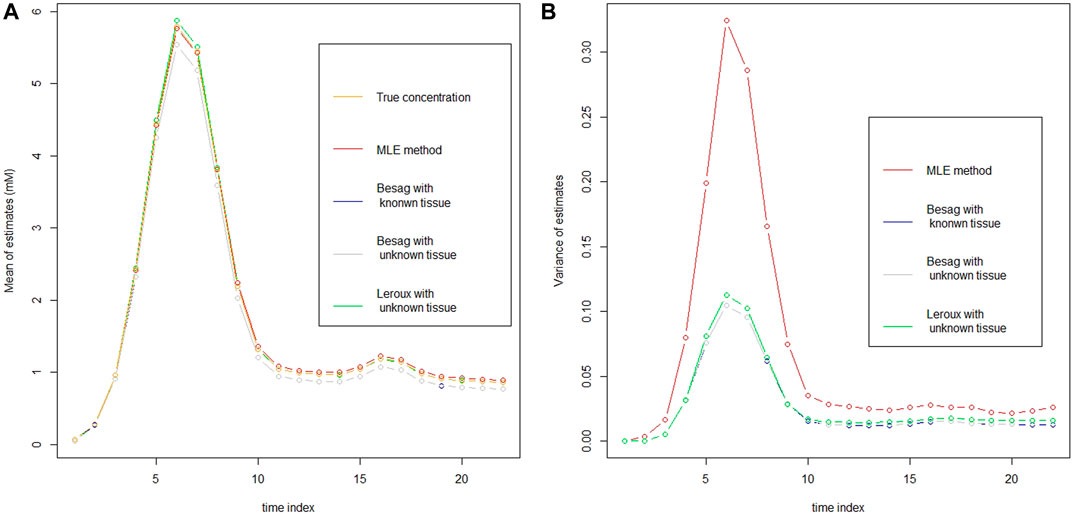
FIGURE 1. Mean (A) and variance (B) of the estimator from each model in vessels as well as the true CA concentration (A) at 3T with rSNR = 5

FIGURE 2

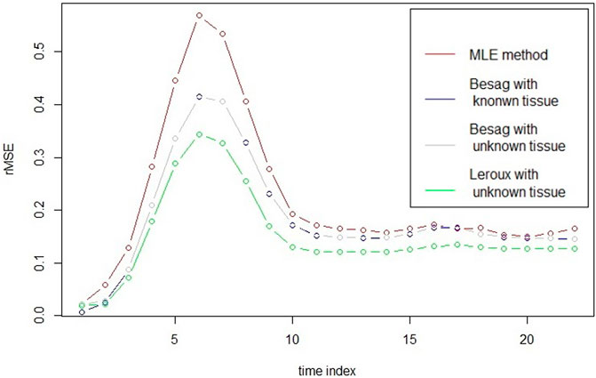
FIGURE 2. rMSE of each model in vessels at 3T with rSNR = 5

From Figure 3, it can be seen that the spatial dependence is negatively associated with CA concentration. The spatial dependence is lower when CA concentration is around the peak and the spatial dependence is getting higher when CA concentration is lower.

FIGURE 3

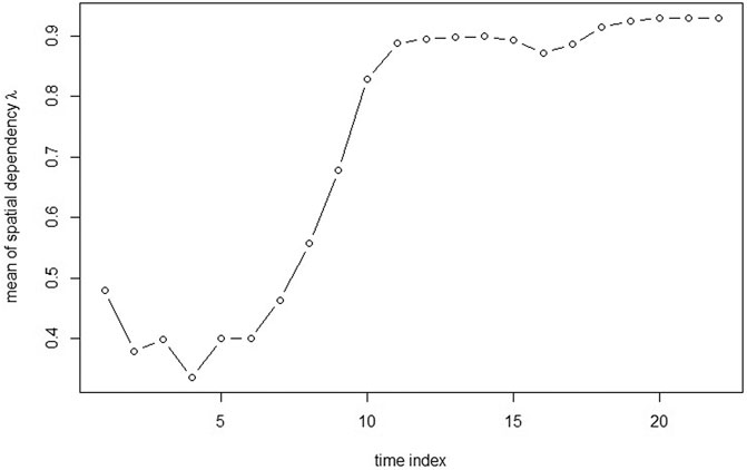
FIGURE 3. Time series of the mean of spatial dependence λ at 3T with rSNR = 5

4.2 Larger Images

Since the smallest averaged $\widehat{\tau }$ for smaller images over all the time points is 0.9, $\widehat{\tau }=0.1$ is selected to minimise Eq. 7 for larger images. The same values shown in Figure 3 are used for $\widehat{\lambda }$ to minimise Eq. 7. From Figure 4, it shows both improvements around the peak and right tail for MAP estimators compared to MLEs over 50 simulations, even though ${\widehat{\sigma }}^2$s are not the optimal ones to minimise c over time points.

FIGURE 4

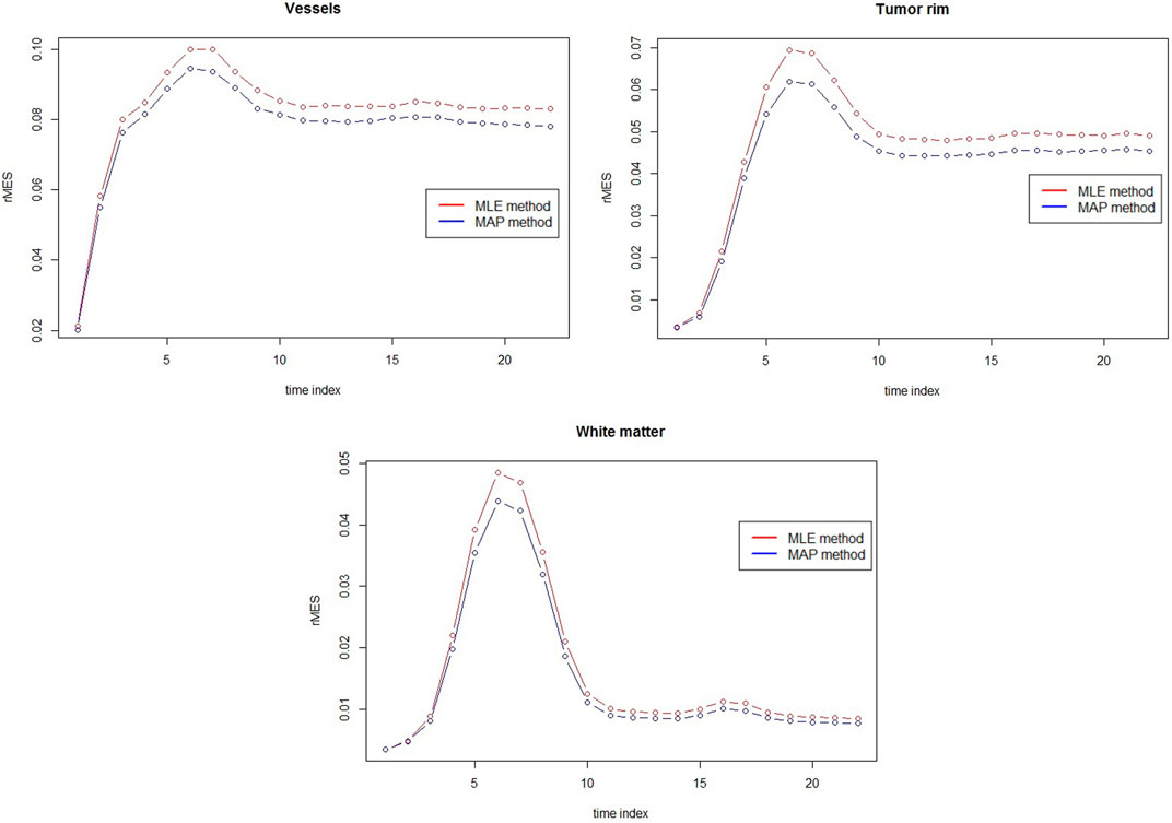
FIGURE 4. rMSE comparison between MAP estimators and MLEs for vessels, tumor rim and white matter at 3T with rSNR = 5 over 50 simulations.

The same analysis is carried out for the data generated with rSNR = 1 at 3T. It shows that λ has similar patten as in Figure 3. $\widehat{\tau }=0.01$, which is less than 0.1, is selected for rSNR = 1 at 3T.

The comparison between MAP estimators and MLEs for three different tissues with respect to rMSE are presented in Figure 5. Clear rMSE reduction by using MAPs can observed. Note that in general the rMSE in Figure 5 is larger than the one in Figure 4 due to the different noise levels.

FIGURE 5

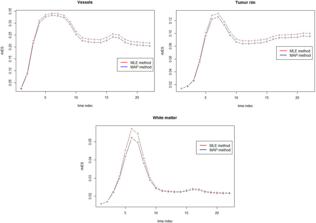
FIGURE 5. rMSE comparison between MAP estimators and MLEs for vessels, tumor rim and white matter at 3T with rSNR = 1 over 50 simulations.

5 Conclusion and Discussion

The investigation in this paper has demonstrated that spatial statistical modelling approaches are capable to improve contrast agent quantification in dynamic contrast enhanced MRI, by utilising the spatial dependence information among image voxels. Bayesian hierarchical models, in particular Besag and Leroux models, have provided notable improvements on CA concentration estimation. Substantial reduction of rMSE in estimation has been obtained by using BHMs in vessels for smaller images. Thereinto, Leroux model outperforms Besag models with two different dependence structures.

For larger images, since the BHMs could not be adopted due to the computational capability, MAP method with the estimated parameters from smaller images is employed to estimate the CA concentration. Our proposed MAP estimators have shown clear improvements, compared to the existing MLE method, on rMSE for vessels, tumor rim and white matter.

Although the smaller images are not practical in clinic, the results showed clear evidences that incorporating borrowing strength from neighbours can improve the accuracy of CA concentration. Further investigation could be done in the future by developing own codes to implement BHMs for larger images instead of using R-INLA. In this case, with Eq. 1 and (2*) as the data model, Leroux model as the process model, one can check if the spatial dependence is invariant or not and how τ changes over different image sizes. Also different magnetic strength, e.g.1.5T, and more rSNRs can be analysed as in Brynolfsson et al. (2014).

The other restriction of this study is that the time dependence was not considered which resulted in a relatively simple statistical model and fast computational time. In reality, it is very reasonable to incorporate time dependence into the BHMs, which is called spatiotemporal BHMs (Cressie and Wikle, 2011). Figure 6 illustrates the spatiotemporal idea in a much concise way.

FIGURE 6

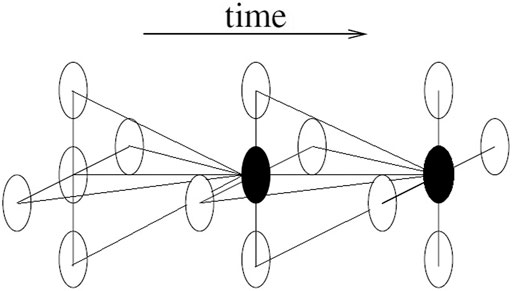
FIGURE 6. Neighbourhood structure in spatiotemporal model.

In Figure 6, the black dot is not only affected by its neighbours in space domain, but also by its neighbours in time domain. Many time series models can be used here, e. g random work models and autoregressive models. By incorporating the time dependence, besides temporal trend, the interaction between spatial and temporal effects can also be studied.

Data Availability Statement

The original contributions presented in the study are included in the article/Supplementary Material, further inquiries can be directed to the corresponding author.

Author Contributions

All authors made significant contributions to the manuscript. JW conducted the statistical analysis and wrote the paper; AG and PB simulated the MRI data and provided knowledge supports in the MRI field. JY supervised the work including writing, reviewing and editing.

Funding

This work was supported by the Swedish Research Council grant (Reg.No. 340-2013-5342).

Conflict of Interest

The authors declare that the research was conducted in the absence of any commercial or financial relationships that could be construed as a potential conflict of interest.

Publisher’s Note

All claims expressed in this article are solely those of the authors and do not necessarily represent those of their affiliated organizations, or those of the publisher, the editors and the reviewers. Any product that may be evaluated in this article, or claim that may be made by its manufacturer, is not guaranteed or endorsed by the publisher.

Acknowledgments

We would like to thank the High Performance Computing Center North (HPC2N) and the Swedish National Infrastructure for Computing (SNIC) for providing the computing resource. We acknowledge the reviewers for their detailed and insightful comments and suggestions that helped to improve the quality of the paper.

References

Assunção, R., and Krainski, E. (2009). Neighborhood Dependence in Bayesian Spatial Models. Biometrical J. 51, 851–869. doi:10.1002/bimj.200900056

CrossRef Full Text | Google Scholar

Atkinson, K. E. (1989). An Introduction to Numerical Analysis. John Wiley & Sons.

Google Scholar

Aubert-Broche, B., Evans, A. C., and Collins, L. (2006). A New Improved Version of the Realistic Digital Brain Phantom. NeuroImage 32, 138–145. doi:10.1016/j.neuroimage.2006.03.052

PubMed Abstract | CrossRef Full Text | Google Scholar

Besag, J. (1974). Spatial Interaction and the Statistical Analysis of Lattice Systems. J. R. Stat. Soc. Ser. B (Methodological) 36, 192–236. doi:10.1111/j.2517-6161.1974.tb00999.x

CrossRef Full Text | Google Scholar

Besag, J., York, J., and Annie, M. (1991). Bayesian Image Restoration, with Two Applications in Spatial Statistics. Ann. Inst. Stat. Maths. 43, 1–20. doi:10.1007/bf00116466

CrossRef Full Text | Google Scholar

Brynolfsson, P., Yu, J., Wirestam, R., Karlsson, M., and Garpebring, A. (2014). Combining Phase and Magnitude Information for Contrast Agent Quantification in Dynamic Contrast-Enhanced MRI Using Statistical Modeling. Magn. Reson. Med. 74, 1156–1164. doi:10.1002/mrm.25490

PubMed Abstract | CrossRef Full Text | Google Scholar

Cao, Y. (2011). The Promise of Dynamic Contrast-Enhanced Imaging in Radiation Therapy. Semin. Radiat. Oncol. 21, 147–156. doi:10.1016/j.semradonc.2010.11.001

PubMed Abstract | CrossRef Full Text | Google Scholar

Cheng, H.-L. M. (2007). T1 Measurement of Flowing Blood and Arterial Input Function Determination for Quantitative 3D T1-Weighted DCE-MRI. J. Magn. Reson. Imaging 25, 1073–1078. doi:10.1002/jmri.20898

CrossRef Full Text | Google Scholar

Cousineau, D., and Hélie, S. (2013). Improving Maximum Likelihood Estimation with Prior Probabilities: a Tutorial on Maximum A Posteriori Estimation and an Examination of the Weibull Distribution. Tutorials Quantitative Methods Psychol. 9, 61–71. doi:10.20982/tqmp.09.2.p061

CrossRef Full Text | Google Scholar

Cressie, N., and Wikle, C. K. (2011). Statistics for Spatio-Temporal Data. Wiley.

Google Scholar

Lee, D. (2011). A Comparison of Conditional Autoregressive Models Used in Bayesian Disease Mapping. Spat. Spatio-temporal Epidemiol. 2, 79–89. doi:10.1016/j.sste.2011.03.001

PubMed Abstract | CrossRef Full Text | Google Scholar

Leroux, B. G., Lei, X., and Breslow, N. (2000). Estimation of Disease Rates in Small Areas: A New Mixed Model for Spatial Dependence. Springer New York, 179–191. chap. Statistical Models in Epidemiology, the Environment, and Clinical Trials. doi:10.1007/978-1-4612-1284-3_4

CrossRef Full Text | Google Scholar

MacNab, Y. C. (2010). On Gaussian Markov Random fields and Bayesian Disease Mapping. Stat. Methods Med. Res. 20, 49–68. doi:10.1177/0962280210371561

PubMed Abstract | CrossRef Full Text | Google Scholar

Reber, D. L. (1999). Inference for Extremes with Applications to Animal Breeding and Disease Mapping. Retrospective Theses and Dissertations, 12160.

Google Scholar

Rinck, P. A. (2019). Magnetic Resonance in Medicine. Norderstedt, Germany: European Magnetic Resonance Forum. Chapter 13.

Google Scholar

Rue, H., and Held, L. (2005). Gaussian Markov Random Fields : Theory and Applications. Boca Raton, FL: Chapman & Hall/CRC.

Google Scholar

Rue, H., Martino, S., and Chopin, N. (2009). Approximate Bayesian Inference for Latent Gaussian Models by Using Integrated Nested Laplace Approximations. J. R. Stat. Soc. Ser. B 71, 319–392. doi:10.1111/j.1467-9868.2008.00700.x

CrossRef Full Text | Google Scholar

Sourbron, S. P., and Buckley, D. L. (2013). Classic Models for Dynamic Contrast-Enhanced MRI. NMR Biomed. 26, 1004–1027. doi:10.1002/nbm.2940

PubMed Abstract | CrossRef Full Text | Google Scholar

Sourbron, S. P., and Buckley, D. L. (2011). Tracer Kinetic Modelling in MRI: Estimating Perfusion and Capillary Permeability. Phys. Med. Biol. 57, R1–R33. doi:10.1088/0031-9155/57/2/r1

PubMed Abstract | CrossRef Full Text | Google Scholar

Stern, H. S., and Cressie, N. (2000). Posterior Predictive Model Checks for Disease Mapping Models. Stat. Med. 19, 2377–2397. doi:10.1002/1097-0258(20000915/30)19:17/18<2377:aid-sim576>3.0.co;2-1

PubMed Abstract | CrossRef Full Text | Google Scholar

Tofts, P. S. (1997). Modeling Tracer Kinetics in Dynamic Gd-DTPA MR Imaging. J. Magn. Reson. Imaging 7, 91–101. doi:10.1002/jmri.1880070113

CrossRef Full Text | Google Scholar

Verma, S., Turkbey, B., Muradyan, N., Rajesh, A., Cornud, F., Haider, M. A., et al. (2012). Overview of Dynamic Contrast-Enhanced MRI in Prostate Cancer Diagnosis and Management. Am. J. Roentgenology 198, 1277–1288. doi:10.2214/ajr.12.8510

CrossRef Full Text | Google Scholar