Distributed Proximal Splitting Algorithms with Rates and Acceleration

1 Introduction

We propose new algorithms for the generic convex optimization problem:

$\underset{x\in \mathcal{X}}{minimize}\left\{\mathrm{\Psi }(x):=\frac{1}{M}\sum _{m=1}^M\left(F_m(x)+H_m(K_{m}x)\right)+R(x)\right\},(1)$

where M ≥ 1 is typically the number of parallel computing nodes in a distributed setting; the $K_m:\mathcal{X}\to {\mathcal{U}}_m$ are linear operators; $\mathcal{X}$ and ${\mathcal{U}}_m$ are real Hilbert spaces (all spaces are supposed of finite dimension); R and H_m are proper, closed, convex functions with values in $\mathbb{R}\cup \{+\infty \}$, the proximity operators of which are easy to compute; and the F_m are convex $L_{F_m}$-smooth functions; that is ∇F_m is $L_{F_m}$-Lipschitz continuous, for some $L_{F_m}>0$.

This template problem covers most convex optimization problems met in signal and image processing, operations research, control, machine learning, and many other fields, and our goal is to propose new generic distributed algorithms able to deal with nonsmooth functions using their proximity operators, with acceleration in presence of strong convexity.

1.1 Contributions

Our contributions are the following:

(1) New algorithms: We propose the first distributed algorithms to solve (Eq. 1) in whole generality, with proved convergence to an exact solution, and having the full splitting, or decoupling, property: ∇F_m, ${\mathrm{p}\mathrm{r}\mathrm{o}\mathrm{x}}_{H_m}$, K_m and $K_m^{*}$ are applied at the m-th node, and the proximity operator of R is applied at the master node connected to all others. No other more complicated operation, like an inner loop or a linear system to solve, is involved.

(2) Unified framework: The foundation of our distributed algorithms consists in two general principles, applied in a cascade, which are new contributions in themselves and could be used in other contexts:

(a) We show that problem (Eq. 1) with M = 1, i.e. the minimization of F + R + H◦K, can be reformulated as the minimization of $\tilde{F}+\tilde{R}+\tilde{H}$ in a different space, with preserved smoothness and strong convexity properties. Hence, the linear operator disappears and the Davis–Yin algorithm (Davis and Yin, 2017) can be applied to this new problem. Through this lens, we recover many algorithms as particular cases of this unified framework, like the PD3O, Chambolle–Pock, Loris–Verhoeven algorithms.

(b) We design a non-straightforward lifting technique, so that the problem (Eq. 1), with any M, is reformulated as the minimization of $\widehat{F}+\widehat{R}+\widehat{H}◦\widehat{K}$ in some product space.

(3) New convergence analysis and acceleration: Even when M = 1, we improve upon the state of the art in two ways:

(a) For constant stepsizes, we recover existing algorithms, but we provide new, more precise, results about their convergence speed, see Theorem 1 and Theorem 5.

(b) With a particular strategy of varying stepsizes, we exhibit new algorithms, which are accelerated versions of them. We prove O(1/k²) convergence rate on the last iterate, see Theorem 3 and Theorem 4, whereas current results in the literature are ergodic, e.g. Chambolle and Pock (2016b).

1.2 Related Work

Many estimation problems in a wide range of scientific fields can be formulated as large-scale convex optimization problems (Palomar and Eldar, 2009; Sra et al., 2011; Bach et al., 2012; Bubeck, 2015; Polson et al., 2015; Chambolle and Pock, 2016a; Glowinski et al., 2016; Stathopoulos et al., 2016; Condat, 2017a; Condat et al., 2019b). Proximal splitting algorithms (Combettes and Pesquet, 2010; Boţ et al., 2014; Parikh and Boyd, 2014; Komodakis and Pesquet, 2015; Beck, 2017; Condat et al., 2019a) are particularly well suited to solve them; they consist of simple, easy to compute, steps that can deal with the terms in the objective function separately.

These algorithms are generally designed as sequential ones, for M = 1, and then they can be extended by lifting in product space to parallel versions, well suited to minimize F + R + ∑_mH_m ○ K_m, see for instance Condat et al., 2019a, Section 8. However, it is not straightforward to adapt lifting to the case of a finite-sum $F=\frac{1}{M}{\sum }_m{F}_m$, with each function F_m handled by a different node, which is of primary importance in machine learning. This generalization is one of our contributions.

There is a vast literature on distributed optimization to minimize $\frac{1}{M}{\sum }_m{F}_m+R$, with a focus on strategies based on (block-)coordinate or randomized activation, as well as replacing the gradients by cheaper stochastic estimates (Cevher et al., 2014; Richtárik and Takáč, 2014; Gorbunov et al., 2020; Salim et al., 2020). Replacing the full gradient by a stochastic oracle in the accelerated algorithms with varying stepsizes we propose is not straightforward; we leave this direction for future research. In any case, the generalized setting, with the smooth functions F_m at the nodes supplemented or replaced by nonsmooth functions H_m, possibly composed with linear operators, seems to have received little attention. We want to make up for that. Decentralized optimization over networks is an active research topic (Latafat et al., 2019; Alghunaim et al., 2021). In this paper, we focus on the centralized client–server model, with one master node connected to several client nodes, working in parallel. We leave the study of decentralized algorithms for future work.

When M = 1 and K = I, where I denotes the identity, Davis and Yin (2017) proposed an efficient algorithm, along with an extensive study of its convergence rates and possible accelerations. But the ability to handle a nontrivial K is behind the success of the Chambolle and Pock (2011) or \Condat (2013), Vũ (2013): they are well suited for regularized inverse problems in imaging (Chambolle and Pock, 2016a), for instance with the total variation and its variants (Bredies et al., 2010; Condat, 2014, 2017b; Duran et al., 2016); other examples are computer vision problems (Cremers et al., 2011), overlapping group norms for sparse estimation in data science (Bach et al., 2012), and trend filtering on graphs (Wang et al., 2016). Another prominent case is when H is an indicator function, so that the problem becomes: minimize F(x) + R(x) subject to Kx = b. If K is a gossip matrix like the minus graph Laplacian, decentralized optimization over a network can be tackled (Shi et al., 2015; Scaman et al., 2017; Salim et al., 2021).

When M = 1 and K is arbitrary, there exist algorithms to solve (Eq. 1) in full generality, for example, the Combettes and Pesquet (2012), Condat, (2013), Vũ (2013), PD3O (Yan, 2018) and PDDY (Salim et al., 2020) algorithms. However, their convergence rates and possible accelerations are little understood. Our main contribution is to derive new convergence rates and accelerated versions of the PD3O and PDDY algorithms, and their particular cases, including Chambolle and Pock (2011) and Loris and Verhoeven (2011) algorithms. In order to do this, we show that these two algorithms can be viewed as instances of the Davis–Yin algorithm. This reformulation technique is inspired by the recent one of O’Connor and Vandenberghe (O’Connor and Vandenberghe, 2020); it makes it possible to split the composition H°K and to derive algorithms, which call the operators prox_H, K, K* separately. This technique is fundamentally different from the one in Salim et al. (2020), showing that the PD3O and PDDY algorithms are primal–dual instances of the operator version of Davis–Yin splitting to solve monotone inclusions. Notably, we can derive convergence rates with respect to the objective function and accelerations, which is not possible with the primal–dual reformulation of Salim et al. (2020). On the other hand, the latter encompasses the Condat–Vũ algorithm (Condat, 2013; Vũ, 2013), which is not the case of our approach. So, these are complementary interpretations.

1.3 Organization of the paper

In Section 2, we propose new nonstationary versions (i.e. with varying stepsizes) of several algorithms for optimization problems made of three terms, and we analyze their convergence rates. The derivation details are pushed to the end of the paper in Section 5 for ease of reading. In Section 3, we further propose distributed algorithms, which can minimize the sum of an arbitrary number of terms. Again, the derivation details are deferred to Section 6. Numerical experiments illustrating the good match between our theoretical results and practical performance are shown in Section 4.

2 Minimization of 3 Functions With a Linear Operator

Let us focus on the problem (Eq. 1) when M = 1:

${minimize}_{x\in \mathcal{X}}\mathrm{\Psi }(x)=F(x)+R(x)+H(Kx),(2)$

where $K:\mathcal{X}\to \mathcal{U}$ is a linear operator, $\mathcal{X}$ and $\mathcal{U}$ are real Hilbert spaces, R and H are proper, closed, convex functions, and F is a convex and L_F-smooth function. We will see in Section 3 that using an adequate lifting technique, (2) can be extended to (1) and, accordingly, parallel or distributed versions of the sequential algorithms to solve (Eq. 2) will be derived. That is why we first study the case M = 1. For any function G, we denote by μ_G ≥ 0 some constant such that G is μ_G-strongly convex; that is, G − (μ_G/2)‖ ⋅‖² is convex.

The dual problem to (Eq. 2) is

${minimize}_{u\in \mathcal{U}}{(F+R)}^{*}(-K^{*}u)+H^{*}(u),(3)$

where K* is the adjoint operator of K and G* is the convex conjugate of a function G (Bauschke and Combettes, 2017); we recall the Moreau identity: ${\mathrm{p}\mathrm{r}\mathrm{o}\mathrm{x}}_{\tau G}(z)=z-\tau {\mathrm{p}\mathrm{r}\mathrm{o}\mathrm{x}}_{G^{*}/\tau }(z/\tau )$ (Bauschke and Combettes, 2017). We suppose that the following holds:

Assumption 1There exists $x^{*}\in \mathcal{X}$ such that 0 ∈ ∇F(x^*) + ∂R(x^*) + K*∂H(Kx^*), which implies that x^* is a solution to (Eq. 2); see for instance Combettes and Pesquet, 2012, Proposition 4.3 for sufficient conditions on the functions for this property to hold.

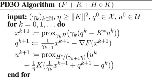
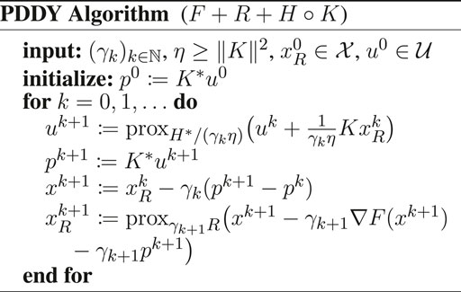
2.1 Deriving the Nonstationary PD3O and PDDY Algorithms

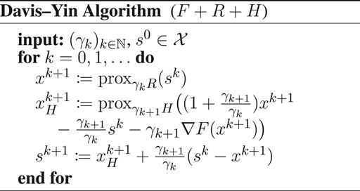
The main difficulty in (Eq. 2) is the presence of the linear operator K. Indeed, if K = I, the Davis–Yin algorithm (Davis and Yin, 2017) is well suited to minimize F + R + H. Note that there is a minor mistake in the way Algorithm 3 in Davis and Yin (2017) is initialized. This is corrected here. Thus, the Davis–Yin algorithm is as follows:

Let ${({\gamma }_k)}_{k\in \mathbb{N}}$ be a sequence of stepsizes. Let $x_H^0\in \mathcal{X}$ and $u^0\in \mathcal{X}$. For k = 0, 1, … iterate

$\lfloor \begin{array}{c}{x}^{k+1}={\mathrm{p}\mathrm{r}\mathrm{o}\mathrm{x}}_{{\gamma }_{k}R}(x_H^k+{\gamma }_k{u}^k)\hfill \\ u^{k+1}=u^k+\frac{1}{{\gamma }_k}(x_H^k-x^{k+1})\hfill \\ x_H^{k+1}={\mathrm{p}\mathrm{r}\mathrm{o}\mathrm{x}}_{{\gamma }_{k+1}H}\left(x^{k+1}-{\gamma }_{k+1}{u}^{k+1}-{\gamma }_{k+1}\nabla F(x^{k+1})\right).\hfill \end{array}(4)$

To make this algorithm applicable to K ≠ I, we reformulate the problem (Eq. 2) as follows:

(1) We choose a value η ≥‖K‖²; we recommend to set η = ‖K‖² in practice. Then there exists a real Hilbert space $\mathcal{W}$ and a linear operator $C:\mathcal{W}\to \mathcal{U}$ such that KK* + CC* = ηI. C is not unique, for instance, we can set $C={(\eta I-K{K}^{*})}^{1/2}$. We actually don’t need to exhibit C, its existence is sufficient here and there will be no call to C in the algorithms.

(2) Now, the problem (Eq. 2) can be rewritten as:

${minimize}_{x\in \mathcal{X},w\in \mathcal{W}}\tilde{F}(x,w)+\tilde{R}(x,w)+\tilde{H}(x,w),(5)$

where $\tilde{F}:(x,w)\mapsto F(x)+\frac{{\mu }_F}{2}\Vert w{\Vert }^2$, $\tilde{R}:(x,w)\mapsto R(x)+{ı}_0(w)$, where ${ı}_0:w\mapsto \left\{0\right.$ if w = 0, + ∞ otherwise}, and $\tilde{H}:(x,w)=H(Kx+Cw)$. Indeed, we introduce the variable w, but also the constraint that w = 0. Since $\tilde{F}(x,0)=F(x)$, $\tilde{R}(x,0)=R(x)$, $\tilde{H}(x,0)=H(Kx)$, the equivalence between (2) and (5) follows.

We have $\nabla \tilde{F}(x,w)=(\nabla F(x),{\mu }_{F}w)$, ${\mathrm{p}\mathrm{r}\mathrm{o}\mathrm{x}}_{\tilde{R}}(x,w)=({\mathrm{p}\mathrm{r}\mathrm{o}\mathrm{x}}_R(x),0)$. Most importantly, for every γ > 0, we have (O’Connor and Vandenberghe, 2020):

${\mathrm{p}\mathrm{r}\mathrm{o}\mathrm{x}}_{{\tilde{H}}^{*}/\gamma }(x,w)=(K^{*}u,C^{*}u),\text{where}u={\mathrm{p}\mathrm{r}\mathrm{o}\mathrm{x}}_{H^{*}/(\gamma \eta )}\left((Kx+Cw)/\eta \right).(6)$

Note that in O’Connor and Vandenberghe (2020), the authors use $\tilde{F}(x,w)=F(x)$, whereas we add $\frac{{\mu }_F}{2}\Vert w{\Vert }^2$. This difference is essential, so that $\tilde{F}$ is L_F-smooth and μ_F-strongly convex. Also, $\tilde{R}$ is μ_R-strongly convex.

Then, we can apply the Davis–Yin algorithm (4) to solve the problem (Eq. 5). We set F, R, H in (Eq. 4) as $\tilde{F}$, $\tilde{R}$, $\tilde{H}$, respectively. The details of the substitutions yielding the algorithms are deferred to Section 5 for the convenience of reading; most notably, whenever CC* appears, it is replaced by ηI − KK*. The obtained algorithms turns out to be a nonstationary version of the PD3O algorithm (Yan, 2018), shown above. On the other hand, if we exchange the two functions and set F, R, H in (Eq. 4) as $\tilde{F}$, $\tilde{H}$, $\tilde{R}$, we obtain a different algorithm. It turns out to be a nonstationary version of the PDDY algorithm proposed recently (Salim et al., 2020), shown above too. With constant stepsizes γ_k ≡ γ ∈ (0, 2/L_F), for both the PD3O and PDDY algorithms, x^k and u^k converge to some solutions x^* and u^* of (Eq. 2) and (Eq. 3), respectively; this result was known for η > ‖K‖² (Yan, 2018; Salim et al., 2020) and shown for η = ‖K‖² for the PD3O algorithm in O’Connor and Vandenberghe (2020), but convergence with η = ‖K‖² for the PDDY algorithm, as stated in Theorem 2, is new.

Particular cases of the PD3O and PDDY algorithms, which are shown above, are the following:

(1) If K = I and η = 1, the PD3O algorithm reverts to the Davis–Yin algorithm (Eq. 4); the PDDY algorithm too, but with H and R exchanged in (Eq. 4).

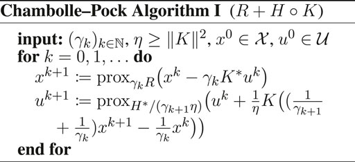
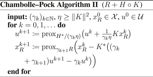
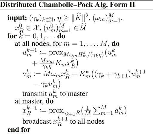
(2) If F = 0, the PD3O and PDDY algorithms revert to the forms I and II (Condat et al., 2019a) of the Chambolle–Pock algorithm, a.k.a. Primal–Dual Hybrid Gradient algorithm (Chambolle and Pock, 2011), respectively.

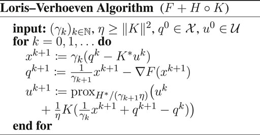
(3) If R = 0, the PD3O and PDDY algorithms revert to the Loris–Verhoeven algorithm (Loris and Verhoeven, 2011), also discovered independently as the PDFP2O (Chen et al., 2013) and PAPC (Drori et al., 2015) algorithms; see also Combettes et al. (2014); Condat et al. (2019a) for an analysis as a primal–dual forward–backward algorithm.

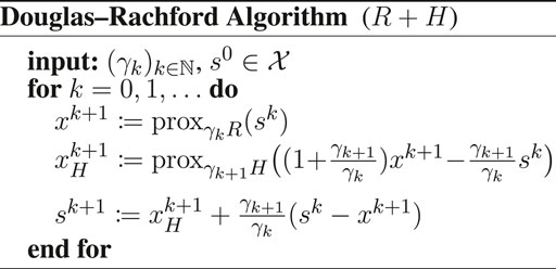
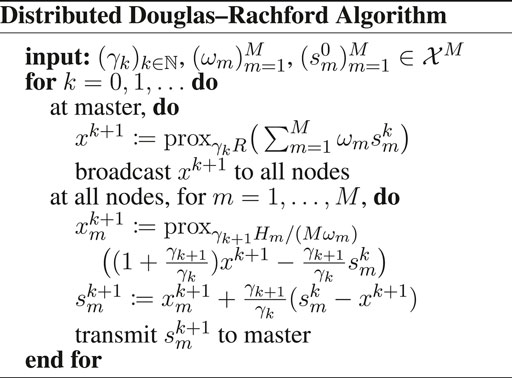
(4) If F = 0 in the Davis–Yin algorithm or K = I and η = 1 in the Chambolle–Pock algorithm, we obtain the Douglas–Rachford algorihm; it is equivalent to the ADMM, see the discussion in Condat et al. (2019a).

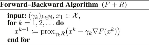
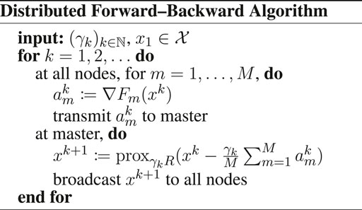
(5) If H = 0, the PD3O and PDDY algorithms revert to the forward–backward algorithm, a.k.a. proximal gradient descent. The Loris–Verhoeven algorithm with K = I and η = 1, too.

2.2 Convergence Analysis

We first give convergence rates for the PD3O algorithm with constant stepsizes.

Theorem 1. (convergence rate of the PD3O algorithm). In the PD3O algorithm, suppose that γ_k ≡ γ ∈ (0, 2/L_F) and η ≥‖K‖². Then x^k and u^k converge to some solutions x^* and u^* of (2) and (3), respectively. In addition, suppose that H is continuous on an open ball centered at Kx^*. Then the following hold:

$(\mathrm{i})\mathrm{\Psi }(x^k)-\mathrm{\Psi }(x*)=o(1/\sqrt{k}).$

Define the weighted ergodic iterate ${\bar{x}}^k=\frac{2}{k(k+1)}{\sum }_{i=1}^{k}i{x}^i$, for every k ≥ 1. Then

$(\mathrm{i}\mathrm{i})\mathrm{\Psi }({\bar{x}}^k)-\mathrm{\Psi }(x*)=O(1/k).$

Furthermore, if H is L-smooth for some L > 0, we have a faster decay for the best iterate so far:

$(\mathrm{i}\mathrm{i}\mathrm{i})\underset{i=1,\dots ,k}{\min }\mathrm{\Psi }(x^i)-\mathrm{\Psi }(x*)=o(1/k).$

Proof. The convergence of x^k follows from Davis and Yin, 2017, Theorem 2.1 and the convergence of u^k follows from the one of the variable $u_B^k=(z^k-x_A^k)/\gamma$ in the notations of Davis and Yin (2017). (i) follows from Davis and Yin, 2017, Theorem 3.1, using the following facts; first, in this theorem, the function corresponding to $\tilde{H}$ is supposed to be Lipschitz-continuous on a certain ball, but since the rate is asymptotic and Kx^k → Kx^*, it is sufficient to consider the property around Kx^*; second, it is well known that if a convex real-valued function is continuous on a convex open set, it is Lipschitz-continuous on every compact subset of this set (Unknown author, 1972); third, if H is continuous, $\tilde{H}$ is continuous too. (ii) follows from Davis and Yin (2017), Theorem 3.2 and (iii) follows from Theorem D.5 in the preprint of Davis and Yin (2017).□

Theorem 1 applies to the particular cases of the PD3O algorithm, like the Loris–Verhoeven, Chambolle–Pock, Douglas–Rachford algorithms. Our results are new even for them.

Remark 1. We can note that the forward–backward algorithm x^k+1 = prox_γR(x^k − γ∇F(x^k)), which is a particular case of the PD3O algorithm when H = 0, is monotonic. So, the best iterate so far is the last iterate. Hence, Theorem 1 (iii) yields Ψ(x^k) − Ψ(x^*) = o(1/k) for the forward–backward algorithm.For the PDDY algorithm, we cannot derive a similar theorem, since $\tilde{R}$ is not continuous around (x^*, 0). Still, we can establish convergence of the variables:

Theorem 2. (convergence of the PDDY algorithm). In the PDDY algorithm, suppose that γ_k ≡ γ ∈ (0, 2/L_F) and η ≥‖K‖². Then x^k and $x_R^k$ both converge to some solution x^* of (Eq. 2), and u^k converges to some solution u^* of (Eq. 3).

Proof. The convergence of x^k and $x_R^k$ to the same solution x^* of (Eq. 2) follows from Davis and Yin, 2017, Theorem 2.1. The convergence of the variable $u_B^k=(z^k-x_A^k)/\gamma$, in the notations of Davis and Yin (2017), implies in our setting, according to (6), that K*u^k and C*u^k both converge to some elements. But since ηu^k = KK*u^k + CC*u^k, u^k converges to some element $u^{*}\in \mathcal{U}$. Finally, we have x^* = prox_γR(x^* − γ∇F(x^*) − γK*u^*), so that 0 ∈ ∂R(x^*) + ∇F(x^*) + K*u^*, and $u^{*}={\mathrm{p}\mathrm{r}\mathrm{o}\mathrm{x}}_{H^{*}/(\gamma \eta )}(u^{*}+\frac{1}{\gamma \eta }K{x}^{*})$, so that Kx^* ∈ (∂H)⁻¹(u^*). Hence, u^* is a solution to (Eq. 3).□

We now give accelerated convergence results using varying stepsizes, when F or R is strongly convex; that is, μ_F + μ_R > 0. In that case, we denote by x^* the unique solution to (Eq. 2).

Theorem 3. (convergence rate of the accelerated PD3O algorithm). Suppose that μ_F + μ_R > 0. Let κ ∈ (0, 1) and γ₀ ∈ (0, 2(1 − κ)/L_F). Set γ₁ = γ₀ and

${\gamma }_{k+1}=\frac{-{\gamma }_k^2{\mu }_F\kappa +{\gamma }_k\sqrt{{({\gamma }_k{\mu }_F\kappa )}^2+1+2{\gamma }_k{\mu }_R}}{1+2{\gamma }_k{\mu }_R},\text{for\hspace{0.17em}every\hspace{0.17em}}k\ge 1.(7)$

Suppose that η ≥‖K‖². Then in the PD3O algorithm, there exists c₀ > 0 (whose expression is given in Section 5) such that, for every k ≥ 1,

$\Vert x^{k+1}-x*{\Vert }^2\le \frac{{\gamma }_{k+1}^2}{1-{\gamma }_{k+1}{\mu }_F\kappa }{c}_0=O\left(1/k^2\right).$

Proof. This result follows from Davis and Yin, 2017, Theorem 3.3, stated for convenience as Lemma 1 in Section 5.□

Note that with the stepsize rule in (Eq. 7), we have k γ_k → 1/(μ_Fκ + μ_R) as k → + ∞, so that γ_k = O(1/k) and γ_k+1/γ_k → 1. Also, when F = 0, L_F can be taken arbitrarily small, so that we can choose any γ₀ > 0.Theorem 3 is new for the PD3O and Loris–Verhoeven algorithms, but has been derived in O’Connor and Vandenberghe (2020) for the Chambolle–Pock algorithm. For the forward–backward algorithm, strong convexity yields linear convergence with constant stepsizes, so this nonstationary version does not seem interesting.Concerning the PDDY algorithm, $\tilde{H}$ is not necessarily strongly convex, even if H is. So, we only consider the case where F is strongly convex. As a consequence of Lemma 1, we get:

Theorem 4. (convergence rate of the accelerated PDDY algorithm). Suppose that μ_F > 0. Let κ ∈ (0, 1) and γ₀ ∈ (0, 2(1 − κ)/L_F). Set γ₁ = γ₀ and

${\gamma }_{k+1}=-{\gamma }_k^2{\mu }_F\kappa +{\gamma }_k\sqrt{{({\gamma }_k{\mu }_F\kappa )}^2+1},\text{for\hspace{0.17em}every\hspace{0.17em}}k\ge 1.(8)$

Suppose that η ≥‖K‖². Then in the PDDY algorithm, there exists c₀ > 0 (whose expression is given in Section 5) such that, for every k ≥ 1,

$\Vert x^{k+1}-x^{*}{\Vert }^2\le \frac{{\gamma }_{k+1}^2}{1-{\gamma }_{k+1}{\mu }_F\kappa }{c}_0=O\left(1/k^2\right).$

Moreover, if η > ‖K‖², $\Vert x_R^k-x^{*}{\Vert }^2=O(1/k^2)$ as well.Finally, we consider the case where, in addition to strong convexity of F or R, H is smooth; in that case, the algorithms with constant stepsizes converge linearly; that is, as a consequence of Lemma 2, we have:

Theorem 5. (linear convergence of the PD3O and PDDY algorithms). Suppose that μ_F + μ_R > 0 and that H is L_H-smooth, for some L_H > 0. Let x^* and u^* be the unique solutions to (2) and (3), respectively. Suppose that γ_k ≡ γ ∈ (0, 2/L_F) and η ≥‖K‖². Then the PD3O algorithm converges linearly: there exists ρ ∈ (0, 1] such that, for every $k\in \mathbb{N}$,

$\begin{array}{ll}\hfill \Vert x^{k+1}-x*{\Vert }^2\le {(1-\rho )}^k& \left(\Vert \gamma q^0-x*+\gamma \nabla F(x*)-\gamma K^{*}(u^0-u*){\Vert }^2\right.\hfill \\ \hfill & \left.+{\gamma }^2\eta \Vert u^0-u*{\Vert }^2-{\gamma }^2\Vert K*(u^0-u^{*}){\Vert }^2\right).\hfill \end{array}$

The PDDY algorithm converges linearly too: there exists ρ ∈ (0, 1] such that, for every $k\in \mathbb{N}$,

$\Vert x_R^{k+1}-x*{\Vert }^2\le 4{(1-\rho )}^k\left(\Vert x_R^0-x*+\gamma K*(u^0-u*){\Vert }^2+{\gamma }^2\eta \Vert u^0-u*{\Vert }^2-{\gamma }^2\Vert K*(u^0-u*){\Vert }^2\right).$

Linear convergence of the other variables in the algorithms can be derived as well, see Proposition 1. Lower bounds for ρ can be derived from Theorem D.6 in the preprint version of Davis and Yin (2017). We don’t provide them, since they are not tight, as noticed in Remark D.2 of the same preprint. For instance, for the PDDY or Loris–Verhoeven algorithms with μ_F > 0,

$\rho =\frac{\gamma {\mu }_F(2-\gamma L_F)}{{(1+\gamma \eta L_H)}^2}.$

If H = 0, by setting L_H = 0, we get ρ = γμ_F(2 − γL_F). But then the PDDY algorithm reverts to the forward–backward algorithm, for which it is known that $1-\rho ={(1-\gamma {\mu }_F)}^2$ whenever γ ≤ 2/(L_F + μ_F), which corresponds to the larger value ρ = γμ_F(2 − γμ_F).We emphasize that linear convergence comes for free with the algorithms, if the conditions are met, without any modification. That is, there is no need to know μ_F, μ_R, L_H, since the conditions on the two parameters γ and η do not depend on these values. For the particular case of the Chambolle–Pock algorithm, as pointed out in O’Connor and Vandenberghe (2020), this is in contrast to existing linear convergence results (Chambolle and Pock, 2016a), derived for a modified version of the algorithm, which depends on these values.

3 Distributed Proximal Algorithms

We now focus on the more general problem (Eq. 1) and we derive distributed versions of the PD3O and PDDY algorithms to solve it. For this, we develop a lifting technique: we recast the minimization of $R(x)+\frac{1}{M}{\sum }_{m=1}^M\left(F_m(x)+H_m(K_{m}x)\right)$ as the minimization of

$\widehat{R}(\widehat{x})+\widehat{F}(\widehat{x})+\widehat{H}(\widehat{K}\widehat{x}),$

as follows. Let ${({\omega }_m)}_{m=1}^M$ be a sequence of positive weights, whose sum is 1; they can be used to mitigate different ‖K_m‖, by setting ω_m ∝ 1/‖K_m‖², or different $L_{F_m}$, by setting ${\omega }_m\propto L_{F_m}^2$, as a rule of thumb.

We introduce the Hilbert space $\widehat{\mathcal{X}}=\mathcal{X}\times \cdots \times \mathcal{X}$ (M times), endowed with the inner product

$\langle \cdot ,{\cdot \rangle }_{\widehat{\mathcal{X}}}:(\widehat{x},{\widehat{x}}^{\prime })\mapsto \sum _{m=1}^M{\omega }_m\langle x_m,x_m^{\prime }\rangle ,$

and the Hilbert space $\widehat{\mathcal{U}}={\mathcal{U}}_1\times \cdots \times {\mathcal{U}}_M$, endowed with the inner product

$\langle \cdot ,{\cdot \rangle }_{\widehat{\mathcal{U}}}:(\widehat{u},{\widehat{u}}^{\prime })\mapsto \sum _{m=1}^M{\omega }_m\langle u_m,u_m^{\prime }\rangle .$

Furthermore, we introduce $\widehat{K}:\widehat{x}={(x_m)}_{m=1}^M\in \widehat{\mathcal{X}}\mapsto (K_1{x}_1,\dots ,K_M{x}_M)\in \widehat{\mathcal{U}}$, and the functions ${ı}_{=}:\widehat{x}\in \widehat{\mathcal{X}}\mapsto \left\{0\right.$ if x₁ = ⋯ = x_M, + ∞ otherwise, $\widehat{R}:\widehat{x}\in \widehat{\mathcal{X}}\mapsto R(x_1)+{ı}_{=}(\widehat{x})$, $\widehat{H}:\widehat{u}\in \widehat{\mathcal{U}}\mapsto \frac{1}{M}{\sum }_{m=1}^M{H}_m(u_m)$, and $\widehat{F}:\widehat{x}\in \widehat{\mathcal{X}}\mapsto \frac{1}{M}{\sum }_{m=1}^M{F}_m(x_m)$. We have to be careful when defining the gradient and proximity operators, because of the weighted metrics; see in Section 6 for details. Doing these substitutions in the PD3O and PDDY algorithms, we obtain the new Distributed PD3O and Distributed PDDY algorithms, shown above. Their particular cases, also shown above, are the distributed

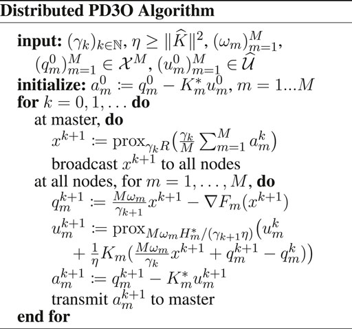
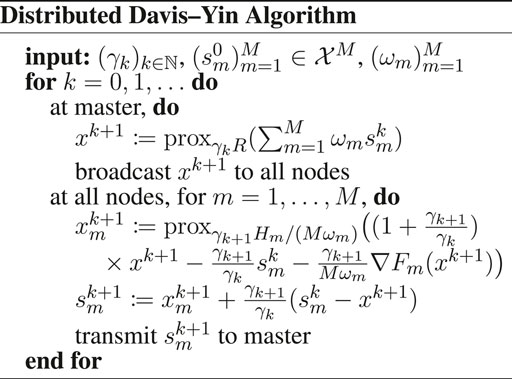
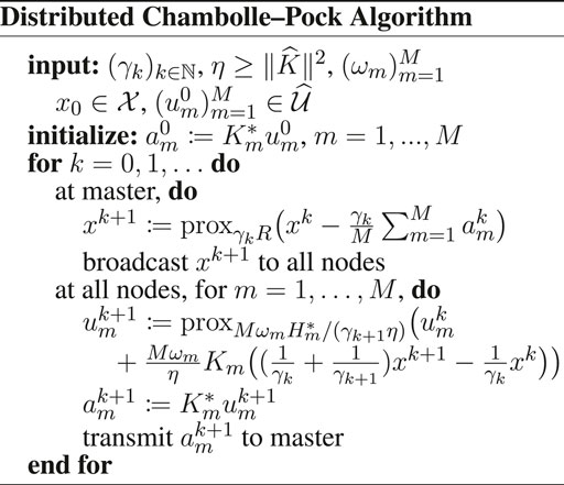
Davis–Yin algorithm when K_m ≡ I and η = 1, the distributed Loris–Verhoeven algorithm when R = 0, the distributed Chambolle–Pock algorithm when F_m ≡ 0, the distributed Douglas–Rachford algorithm when F_m ≡ 0, K_m ≡ I and η = 1, the (classical) distributed forward–backward algorithm when H_m ≡ 0.

We can easily translate Theorems 1–5 to these distributed algorithms; the corresponding theorems are given in Section 6. In a nutshell, we obtain the same convergence results and rates with any number of nodes M ≥ 1 as in the non-distributed setting, for any ${\gamma }_0\in (\mathrm{0,2}/L_{\widehat{F}})$ and $\eta \ge \Vert \widehat{K}{\Vert }^2$, where $L_{\widehat{F}}$ and $\widehat{K}$ are detailed in Section 6. Hence, to our knowledge, we are the first to propose distributed proximal splitting methods with guaranteed, possibly accelerated, convergence, to minimize an arbitrary sum of smooth or nonsmooth functions, possibly composed with linear operators.

4 Experiments

4.1 Image Deblurring Regularized With Total Variation

We first consider the non-distributed problem (Eq. 2), for the imaging inverse problem of deblurring, which consists in restoring an image y corrupted by blur and noise (Chambolle and Pock, 2016a). So, we set

$F:x\mapsto \frac{1}{2}\Vert Ax-y{\Vert }^2,$

where the linear operator A corresponds to a 2-D convolution with a lowpass filter, with L_F = 1. The filter is approximately Gaussian and chosen so that F is μ_F-strongly convex with μ_F = 0.01. y is obtained by applying A to the classical 256 × 256 Shepp–Logan phantom image, with additive Gaussian noise. R = ı₀ enforces nonnegativity of the pixel values. H°K corresponds to the classical ‘isotropic’ total variation (TV) (Chambolle and Pock, 2016a; Condat, 2017b), with H = 0.6 times the l_1,2 norm and K the concatenation of vertical and horizontal finite differences.

We compare the nonaccelerated, i.e. with constant γ_k, and accelerated versions, with decaying γ_k, of the PD3O, PDDY and Condat–Vũ algorithms. We initialize the dual variables at zero and the estimate of the solution as y. We set γ₀ = 1.7, κ = 0.15, η = 8 ≥‖K‖² (except for the accelerated Condat–Vũ algorithm proposed in Chambolle and Pock (2016b), for which η = 16 and γ = 0.5).

The results are illustrated in Figure 1 (implementation in Matlab). We observe that the PD3O and PDDY algorithms have almost identical variables: the pink, red, blue curves are superimposed; we know that both algorithms are identical and revert to the Loris–Verhoeven algorithm when R = 0. Here R ≠ 0 but the nonnegativity constraint does not change the solution significantly, which explains the similarity of the two algorithms.

FIGURE 1

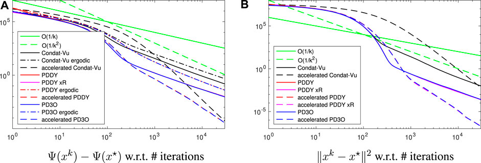
FIGURE 1. Convergence error, in log-log scale, for the experiment of image deblurring regularized with the total variation, see Section 4.1 for details.

Note that x^k in the PDDY algorithm is not feasible with respect to nonnegativity, and the red curve actually shows F(x^k) + H(Kx^k) − Ψ(x^*). In the nonaccelerated case, Ψ(x^k) decays faster than O(1/k) but slower than O(1/k²), which is coherent with Theorem 1. The same holds for $\Vert x^k-x^{*}{\Vert }^2\le \frac{2}{{\mu }_F}(\mathrm{\Psi }(x^k)-\mathrm{\Psi }(x^{*}))$.

The accelerated versions improve the convergence speed significantly: Ψ(x^k) and ‖x^k − x^*‖² decay even faster than O(1/k²), in line with Theorem 3 and Theorem 4. In all cases, the Condat–Vũ algorithm is outperformed. Also, there is no interest in considering the ergodic iterate instead of the last iterate, since the former converges at the same asymptotic rate as the latter, but slower.

4.2 Image Deblurring Regularized With Huber-TV

We consider the same deblurring experiment as before, but we make H smooth by taking the Huber function instead of the l₁ norm in the total variation; that is, λ|⋅| in the latter is replaced by

$h:t\in \mathbb{R}\mapsto \left\{\begin{array}{cc}\frac{\lambda }{2\nu }{t}^2\hfill & \text{if}|t|\le \nu ,\hfill \\ \lambda \left(|t|-\frac{\nu }{2}\right)\hfill & \text{otherwise},\hfill \end{array}\right.$

for some ν > 0 and λ > 0 (set here as 0.1 and 0.6, respectively). We can also write h without branching as $h(t)=\frac{\lambda }{2\nu }\max {(\nu -|t|,0)}^2+\lambda (|t|-\frac{\nu }{2})$. It is known that h is L_h-smooth with L_h = λ/ν. For any γ > 0 and $t\in \mathbb{R}$, we have ${\mathrm{p}\mathrm{r}\mathrm{o}\mathrm{x}}_{h^{*}/\gamma }(t)=t/\max (|t|/\lambda ,1+\frac{\nu }{\lambda \gamma })$. Except for H, everything is unchanged.

The results are illustrated in Figure 2. Again, the PD3O and PDDY algorithms behave very similarly; they converge linearly, as proved in Theorem 5, and achieve machine precision in finite time. x^k in the PDDY algorithm is not feasible and F(x^k) + H(Kx^k) − Ψ(x^*) (red curve) takes negative values (not shown in log scale); so, $x_R^k$ is the variable to study in this setting. We tested the ‘accelerated’ versions of the algorithms with decaying γ_k, but in this scenario, they are much slower and not suitable. Again, the Condat–Vũ algorithm is outperformed and the ergodic sequences converge much slower. Interestingly, the image x^* is visually the same with TV and with Huber-TV.

FIGURE 2

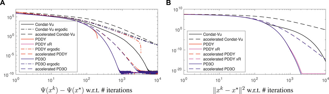
FIGURE 2. Convergence error, in log-log scale, for the experiment of image deblurring regularized with the smooth Huber-total-variation, so that linear convergence occurs, see Section 4.2 for details.

4.3 SVM With Hinge Loss

Here we consider Problem (Eq. 1) in the special case with $\mathcal{X}={\mathbb{R}}^d$, for some d ≥ 1, F_m ≡ 0, and K_m ≡ I; that is, the problem of minimizing

$\mathrm{\Psi }(x)=\frac{1}{M}\sum _{m=1}^M{H}_m(x)+R(x).(9)$

In particular, to train a binary classifier, we consider the classical SVM problem with hinge loss, which has the form (Eq. 9) with $R(x)=\frac{\alpha }{2}\Vert x{\Vert }^2$, for some α > 0, and $H_m(x)=\max (1-b_m{a}_m^{\text{T}}x,0)$, with data samples $a_m\in {\mathbb{R}}^d$ and b_m ∈ { − 1, 1}.

For any γ > 0 we have prox_γR(x) = x/(1 + γα). We could view the dot product $x\mapsto b_m{a}_m^{\text{T}}x$ as a linear operator K_m, but it is more interesting to integrate it in the function H_m. Indeed, as is perhaps not well known, the proximity operator of H_m has a closed form: for any γ > 0,

${\mathrm{p}\mathrm{r}\mathrm{o}\mathrm{x}}_{\gamma H_m}:x\in {\mathbb{R}}^d\mapsto x-\frac{b_m}{{\eta }_m}\max \left(\min (b_m{a}_m^{\text{T}}x-\mathrm{1,0}),-{\eta }_m\gamma \right)a_m,$

where ${\eta }_m=a_m^{\text{T}}{a}_m=\Vert a_m{\Vert }^2$. Thus, we use the Distributed Douglas–Rachford algorithm, a particular case of the distributed PD3O and PDDY algorithms. Since R is α-strongly convex, we also use the accelerated version of the algorithm with varying stepsizes, like in Theorem 3. We can note that in the context of Federated learning (Konečný et al., 2016; Malinovsky et al., 2020), where each m corresponds to the smart phone or computer of a different user with its own data (a_m, b_m) stored locally, the problem is solved in a collaborative way but with preserved privacy, without the users sharing their data.

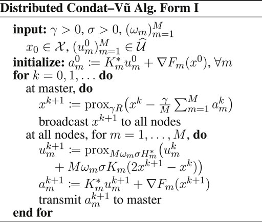
The method was implemented in Python on a single machine and tested on the dataset ‘australian’ from the LibSVM base (Chang and Lin, 2011), with d = 15 and M = 680. We set ω_m ≡ 1/M, α = 0.1, γ₀ = 0.1, and we used zero vectors for the initialization. The results are shown in Figure 3. Despite the oscillations, we observe that both the objective suboptimality and the squared distance to the solution converge sublinearly, with rates looking like $o(1/\sqrt{k})$ and O(1/k²) for the nonaccelerated and accelerated algorithms, respectively, as guaranteed by Theorem 1 and Theorem 3. The proposed accelerated version of the distributed Douglas–Rachford algorithm yields a significant speedup.

FIGURE 3

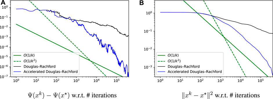
FIGURE 3. Convergence error, in log-log scale, for the SVM binary classification experiment with hinge loss, see Section 4.3 for details.

5 Derivation of the Algorithms

In this section, we give the details of the derivation of the PD3O and PPDY algorithms, and their particular cases, to solve:

$\underset{x\in \mathcal{X}}{minimize}F(x)+R(x)+H(Kx),$

with same notations and assumptions as above. Let η ≥‖K‖², let $\mathcal{W}$ be a real Hilbert space and $C:\mathcal{W}\to \mathcal{U}$ be a linear operator, such that KK^* + CC^* = ηI. We set Q : (x, w)↦Kx + Cw. We have QQ* = ηI. Let ${({\gamma }_k)}_{k\in \mathbb{N}}$ be a sequence of positive stepsizes.

5.1 The Davis–Yin Algorithm

In this section, we state the results on the Davis–Yin algorithm, which we be needed to analyze the PD3O and PPDY algorithms.

The Davis–Yin algorithm to minimize the sum of 3 convex functions $\tilde{F}+G+J$ over a real Hilbert space $\mathcal{Z}$ (assuming that there exists a solution z^* such that $0\in \nabla \tilde{F}(z^{*})+\partial G(z^{*})+\partial J(z^{*})$) is (Davis and Yin, 2017):

Let $z_J^0\in \mathcal{Z}$, $u_G^0\in \mathcal{Z}$. For k = 0, 1, … iterate:

$\lfloor \begin{array}{c}{z}_G^{k+1}={\mathrm{p}\mathrm{r}\mathrm{o}\mathrm{x}}_{{\gamma }_{k}G}(z_J^k+{\gamma }_k{u}_G^k)\hfill \\ u_G^{k+1}=u_G^k+\frac{1}{{\gamma }_k}(z_J^k-z_G^{k+1})\hfill \\ z_J^{k+1}={\mathrm{p}\mathrm{r}\mathrm{o}\mathrm{x}}_{{\gamma }_{k+1}J}\left(z_G^{k+1}-{\gamma }_{k+1}{u}_G^{k+1}-{\gamma }_{k+1}\nabla \tilde{F}(z_G^{k+1})\right).\hfill \end{array}(10)$

Equivalently, introducing the variable $r^k:=z_J^k+{\gamma }_k{u}_G^k$: let $r^0\in \mathcal{Z}$. For k = 0, 1, … iterate:

$\lfloor \begin{array}{c}{z}_G^{k+1}={\mathrm{p}\mathrm{r}\mathrm{o}\mathrm{x}}_{{\gamma }_{k}G}(r^k)\hfill \\ z_J^{k+1}={\mathrm{p}\mathrm{r}\mathrm{o}\mathrm{x}}_{{\gamma }_{k+1}J}\left(\left(1+\frac{{\gamma }_{k+1}}{{\gamma }_k}\right)z_G^{k+1}-\frac{{\gamma }_{k+1}}{{\gamma }_k}{r}^k-{\gamma }_{k+1}\nabla \tilde{F}(z_G^{k+1})\right)\hfill \\ r^{k+1}=z_J^{k+1}+\frac{{\gamma }_{k+1}}{{\gamma }_k}(r^k-z_G^{k+1}).\hfill \end{array}(11)$

Equivalently: let $r^0\in \mathcal{Z}$. For k = 0, 1, … iterate:

$\lfloor \begin{array}{c}{z}_G^{k+1}={\mathrm{p}\mathrm{r}\mathrm{o}\mathrm{x}}_{{\gamma }_{k}G}(r^k)\hfill \\ u_J^{k+1}={\mathrm{p}\mathrm{r}\mathrm{o}\mathrm{x}}_{J^{*}/{\gamma }_{k+1}}\left(\left(\frac{1}{{\gamma }_{k+1}}+\frac{1}{{\gamma }_k}\right)z_G^{k+1}-\frac{1}{{\gamma }_k}{r}^k-\nabla \tilde{F}(z_G^{k+1})\right)\hfill \\ r^{k+1}=z_G^{k+1}-{\gamma }_{k+1}\nabla \tilde{F}(z_G^{k+1})-{\gamma }_{k+1}{u}_J^{k+1}.\hfill \end{array}(12)$

In our notations, Theorem 3.3 of Davis and Yin (2017) translates into Lemma 1 as follows; we assume that $\tilde{F}$ is $L_{\tilde{F}}$-smooth and ${\mu }_{\tilde{F}}$-strongly convex and that G is μ_G-strongly convex, for some $L_{\tilde{F}}>0$, ${\mu }_{\tilde{F}}\ge 0$, μ_G ≥ 0.

Lemma 1. (accelerated Davis–Yin algorithm). Suppose that ${\mu }_{\tilde{F}}+{\mu }_G>0$. Let z^* be the unique minimizer of $\tilde{F}+G+J$; that is, $0\in \nabla \tilde{F}(z^{*})+\partial G(z^{*})+\partial J(z^{*})$. Let $u_G^{*}$ be such that $u_G^{*}\in \partial G(z^{*})$ and $0\in \nabla \tilde{F}(z^{*})+\partial J(z^{*})+u_G^{*}$. Let κ ∈ (0, 1) and ${\gamma }_0\in (\mathrm{0,2}(1-\kappa )/L_{\tilde{F}})$. Set γ₁ = γ₀ and

${\gamma }_{k+1}=\frac{-{\gamma }_k^2{\mu }_{\tilde{F}}\kappa +{\gamma }_k\sqrt{{({\gamma }_k{\mu }_{\tilde{F}}\kappa )}^2+1+2{\gamma }_k{\mu }_G}}{1+2{\gamma }_k{\mu }_G},\text{for\hspace{0.17em}every\hspace{0.17em}}k\ge 1.$

Then, for every k ≥ 1,

$\Vert z_G^{k+1}-z*{\Vert }^2\le \frac{{\gamma }_{k+1}^2}{1-{\gamma }_{k+1}{\mu }_{\tilde{F}}\kappa }{c}_0=O\left(1/k^2\right),$

where

$c_0=\frac{1-{\gamma }_0{\mu }_{\tilde{F}}\kappa }{{\gamma }_0^2}\Vert z_G^1-z^{*}{\Vert }^2+\Vert u_G^1-u_G^{*}{\Vert }^2.$

Note that $u_G^1=(r^0-z_G^1)/{\gamma }_0$.Linear convergence occurs in the following conditions, according to Theorem D.6 in the preprint version of Davis and Yin (2017), which translates into Lemma 2 as follows. We assume that $\tilde{F}$ is $L_{\tilde{F}}$-smooth and ${\mu }_{\tilde{F}}$-strongly convex, G is μ_G-strongly convex, and J is μ_J-strongly convex, for some $L_{\tilde{F}}>0$, ${\mu }_{\tilde{F}}\ge 0$, μ_G ≥ 0, μ_J ≥ 0. We consider constant stepsizes γ_k ≡ γ, for some $\gamma \in (\mathrm{0,2}/L_{\tilde{F}})$.

Lemma 2. (linear convergence of the Davis–Yin algorithm). Suppose that ${\mu }_{\tilde{F}}+{\mu }_G+{\mu }_J>0$ and that G is L_G-smooth, for some L_G > 0, or J is L_J-smooth, for some L_J > 0. Let z^* be the unique minimizer of $\tilde{F}+G+J$; that is, $0\in \nabla \tilde{F}(z^{*})+\partial G(z^{*})+\partial J(z^{*})$. The dual problem of minimizing ${(\tilde{F}+J)}^{*}(-u)+G^{*}(u)$ over $u\in \mathcal{Z}$ is strongly convex too; let $u_G^{*}$ be its unique solution. We have $u_G^{*}\in \partial G(z^{*})$ and $0\in \nabla \tilde{F}(z^{*})+\partial J(z^{*})+u_G^{*}$. Set $r^{*}=z^{*}+\gamma u_G^{*}$. Then, the Davis–Yin algorithm (Eq. 11) converges linearly: there exists ρ ∈ (0, 1] such that, for every $k\in \mathbb{N}$,

$\Vert r^k-r*{\Vert }^2\le {(1-\rho )}^k\Vert r^0-r*{\Vert }^2.(13)$

Loose lower bounds for ρ are given in Davis and Yin, 2017, Theorem D.6.We have the following corollary of Lemma 2:

Proposition 1. (linear convergence of the other variables in the Davis–Yin algorithm). In the same conditions and notations as in Lemma 2, we have, for every $k\in \mathbb{N}$,

$\begin{array}{ll}\hfill \Vert z_G^{k+1}-z*{\Vert }^2& \le {(1-\rho )}^k\Vert r^0-r*{\Vert }^2\hfill \\ \hfill \Vert z_J^{k+1}-z*{\Vert }^2& \le 4{(1-\rho )}^k\Vert r^0-r*{\Vert }^2.\hfill \end{array}(14)$

Also, in the form (Eq. 12) of the algorithm,

$\Vert u_J^{k+1}+uG*+\nabla \tilde{F}(z*){\Vert }^2\le \frac{4}{{\gamma }^2}{(1-\rho )}^k\Vert r^0-r*{\Vert }^2$

and, in the form (Eq. 10) of the algorithm,

$\Vert u_G^{k+1}-uG*{\Vert }^2\le \frac{1}{{\gamma }^2}{(1-\rho )}^k\Vert r^0-r^{*}{\Vert }^2.$

Proof. Let $k\in \mathbb{N}$. By nonexpansiveness of the proximity operator, in view of the first line in (Eq. 11), we have $\Vert z_G^{k+1}-z^{*}\Vert \le \Vert r^k-r^{*}\Vert$, so that (Eq. 14) follows from (Eq. 13). In addition, in view of the second line in (Eq. 11), we have

$\begin{array}{ll}\hfill \Vert z_J^{k+1}-z*{\Vert }^2& \le \Vert 2(z_G^{k+1}-z*)-(r^k-r*)-\gamma (\nabla \tilde{F}(z_G^{k+1})-\nabla \tilde{F}(z*)){\Vert }^2\hfill \\ \hfill & =\Vert (z_G^{k+1}-z*)-(r^k-r*)+(I-\gamma \nabla \tilde{F})(z_G^{k+1})-(I-\gamma \nabla \tilde{F})(z*){\Vert }^2\hfill \\ \hfill & =\Vert (I-{\mathrm{p}\mathrm{r}\mathrm{o}\mathrm{x}}_{\gamma G})(r^k)-(I-{\mathrm{p}\mathrm{r}\mathrm{o}\mathrm{x}}_{\gamma G})(r*)+(I-\gamma \nabla \tilde{F})(z_G^{k+1})-(I-\gamma \nabla \tilde{F})(z*){\Vert }^2\hfill \end{array}$

and, by nonexpansiveness of I − prox_γG and $I-\gamma \nabla \tilde{F}$,

$\begin{array}{ll}\hfill \Vert z_J^{k+1}-z*{\Vert }^2& \le {\left(\Vert r^k-r*\Vert +\Vert z_G^{k+1}-z*\Vert \right)}^2\hfill \\ \hfill & \le 4\Vert r^k-r*{\Vert }^2.\hfill \end{array}$

Using the same arguments, in view of the second line in (Eq. 12),

$\begin{array}{ll}\hfill \Vert u_J^{k+1}+uG*+\nabla \tilde{F}(z*){\Vert }^2& \le \frac{1}{{\gamma }^2}{\left(\Vert r^k-r*\Vert +\Vert z_G^{k+1}-z*\Vert \right)}^2\hfill \\ \hfill & \le \frac{4}{{\gamma }^2}\Vert r^k-r*{\Vert }^2.\hfill \end{array}$

Finally, as visible in the first line of (Eq. 16), since $r^k=z_J^k+{\gamma }_k{u}_G^k$, and using the Moreau identity, we have $u_G^{k+1}={\mathrm{p}\mathrm{r}\mathrm{o}\mathrm{x}}_{G^{*}/\gamma }(\frac{1}{\gamma }{z}_J^k+u_G^k)={\mathrm{p}\mathrm{r}\mathrm{o}\mathrm{x}}_{G^{*}/\gamma }(\frac{1}{\gamma }{r}^k)$, so that

$\Vert u_G^{k+1}-u_G^{*}{\Vert }^2\le \frac{1}{{\gamma }^2}\Vert r^k-r*{\Vert }^2.$

□

5.2 The PD3O Algorithm

We set $\mathcal{Z}=\mathcal{X}\times \mathcal{W}$, $\tilde{F}$, $G=\tilde{R}$, $J=\tilde{H}$, as defined in Section 2. Doing the substitutions in (Eq. 12), we get the algorithm:

Let $s^0\in \mathcal{X}$ and $r_w^0\in \mathcal{W}$. For k = 0, 1, … iterate:

$\lfloor \begin{array}{c}{x}^{k+1}={\mathrm{p}\mathrm{r}\mathrm{o}\mathrm{x}}_{{\gamma }_{k}R}(s^k)\hfill \\ u^{k+1}={\mathrm{p}\mathrm{r}\mathrm{o}\mathrm{x}}_{H^{*}/({\gamma }_{k+1}\eta )}\left(K\left(\left(\frac{1}{{\gamma }_{k+1}}+\frac{1}{{\gamma }_k}\right)x^{k+1}-\frac{1}{{\gamma }_k}{s}^k-\nabla F(x^{k+1})\right)/\eta -C{r}_w^k/({\gamma }_k\eta )\right)\hfill \\ s^{k+1}=x^{k+1}-{\gamma }_{k+1}\nabla F(x^{k+1})-{\gamma }_{k+1}{K}^{*}{u}^{k+1}\hfill \\ r_w^{k+1}=-{\gamma }_{k+1}{C}^{*}{u}^{k+1}.\hfill \end{array}$

We can remove the variable r_w and the algorithm becomes: Let $s^0\in \mathcal{X}$ and $u^0\in \mathcal{U}$. For k = 0, 1, … iterate:

$\lfloor \begin{array}{c}{x}^{k+1}={\mathrm{p}\mathrm{r}\mathrm{o}\mathrm{x}}_{{\gamma }_{k}R}(s^k)\hfill \\ u^{k+1}={\mathrm{p}\mathrm{r}\mathrm{o}\mathrm{x}}_{H^{*}/({\gamma }_{k+1}\eta )}\left(\frac{1}{\eta }K\left(\left(\frac{1}{{\gamma }_{k+1}}+\frac{1}{{\gamma }_k}\right)x^{k+1}-\frac{1}{{\gamma }_k}{s}^k-\nabla F(x^{k+1})\right)+\frac{1}{\eta }CC*u^k\right)\hfill \\ s^{k+1}=x^{k+1}-{\gamma }_{k+1}\nabla F(x^{k+1})-{\gamma }_{k+1}{K}^{*}{u}^{k+1}.\hfill \end{array}$

After replacing CC* by ηI − KK*, the iteration becomes:

$\lfloor \begin{array}{c}{x}^{k+1}={\mathrm{p}\mathrm{r}\mathrm{o}\mathrm{x}}_{{\gamma }_{k}R}(s^k)\hfill \\ u^{k+1}={\mathrm{p}\mathrm{r}\mathrm{o}\mathrm{x}}_{H^{*}/({\gamma }_{k+1}\eta )}\left(u^k+\frac{1}{\eta }K\left(\left(\frac{1}{{\gamma }_{k+1}}+\frac{1}{{\gamma }_k}\right)x^{k+1}-\frac{1}{{\gamma }_k}{s}^k-\nabla F(x^{k+1})-K*u^k\right)\right)\hfill \\ s^{k+1}=x^{k+1}-{\gamma }_{k+1}\nabla F(x^{k+1})-{\gamma }_{k+1}K*u^{k+1}.\hfill \end{array}$

We can change the variables, so that only one call to ∇F and K* appears, which yields the algorithm: Let $q^0\in \mathcal{X}$ and $u^0\in \mathcal{U}$. For k = 0, 1, … iterate:

$\lfloor \begin{array}{c}{x}^{k+1}={\mathrm{p}\mathrm{r}\mathrm{o}\mathrm{x}}_{{\gamma }_{k}R}\left({\gamma }_k(q^k-K^{*}{u}^k)\right)\hfill \\ q^{k+1}=\frac{1}{{\gamma }_{k+1}}{x}^{k+1}-\nabla F(x^{k+1})\hfill \\ u^{k+1}={\mathrm{p}\mathrm{r}\mathrm{o}\mathrm{x}}_{H*/({\gamma }_{k+1}\eta )}\left(u^k+\frac{1}{\eta }K\left(\frac{1}{{\gamma }_k}{x}^{k+1}+q^{k+1}-q^k\right)\right).\hfill \end{array}$

When γ_k ≡ γ is constant, we recover the PD3O algorithm (Yan, 2018).

To derive Theorem 3 from Lemma 1, we simply have to notice that the variable $z_G^{k+1}$ in the latter corresponds to the pair (x^k+1, 0). Also, in the conditions of Theorem 3, let u^* be any solution of (Eq. 3); that is, u^* ∈ ∂H(Kx^*) and 0 ∈ ∂R(x^*) + ∇F(x^*) + K^*u^*. Then the constant c₀ is

$c_0=\frac{1-{\gamma }_0{\mu }_F\kappa }{{\gamma }_0^2}\Vert x^1-x*{\Vert }^2+\Vert q^0-\frac{1}{{\gamma }_0}{x}^1-K^{*}(u^0-u*)+\nabla F(x*){\Vert }^2+\eta \Vert u^0-u*{\Vert }^2-\Vert K^{*}(u^0-u*){\Vert }^2.$

If K = I and η = 1, the PD3O algorithm reverts to the Davis–Yin algorithm, as given in (Eq. 4). In the conditions of Theorem 3, let u^* be any solution of (Eq. 3); that is, u^* ∈ ∂H(x^*) and 0 ∈ ∂R(x^*) + ∇F(x^*) + u^*. Then the constant c₀ is

$c_0=\frac{1-{\gamma }_0{\mu }_F\kappa }{{\gamma }_0^2}\Vert x^1-x*{\Vert }^2+\Vert \frac{1}{{\gamma }_0}(s^0-x^1)+u*+\nabla F(x*){\Vert }^2.(15)$

5.3 The PDDY Algorithm

The PDDY algorithm is obtained like the PD3O algorithm from the David–Yin algorithm, but after swapping the roles of $\tilde{H}$ and $\tilde{R}$.

To obtain the PDDY algorithm, starting from (Eq. 10), let us first write the Davis–Yin algorithm as: Let $z_J^0\in \mathcal{Z}$ and $u_G^0\in \mathcal{Z}$. For k = 0, 1, … iterate:

$\lfloor \begin{array}{c}{u}_G^{k+1}={\mathrm{p}\mathrm{r}\mathrm{o}\mathrm{x}}_{G^{*}/{\gamma }_k}\left(\frac{1}{{\gamma }_k}{z}_J^k+u_G^k\right)\hfill \\ z_G^{k+1}=z_J^k-{\gamma }_k(u_G^{k+1}-u_G^k)\hfill \\ z_J^{k+1}={\mathrm{p}\mathrm{r}\mathrm{o}\mathrm{x}}_{{\gamma }_{k+1}J}\left(z_G^{k+1}-{\gamma }_{k+1}\nabla \tilde{F}(z_G^{k+1})-{\gamma }_{k+1}{u}_G^{k+1}\right).\hfill \end{array}$

Equivalently: Let $r^0\in \mathcal{Z}$. For k = 0, 1, … iterate:

$\lfloor \begin{array}{c}{u}_G^{k+1}={\mathrm{p}\mathrm{r}\mathrm{o}\mathrm{x}}_{G^{*}/{\gamma }_k}(r^k/{\gamma }_k)\hfill \\ z_G^{k+1}=r^k-{\gamma }_k{u}_G^{k+1}\hfill \\ z_J^{k+1}={\mathrm{p}\mathrm{r}\mathrm{o}\mathrm{x}}_{{\gamma }_{k+1}J}\left(z_G^{k+1}-{\gamma }_{k+1}\nabla \tilde{F}(z_G^{k+1})-{\gamma }_{k+1}{u}_G^{k+1}\right)\hfill \\ r^{k+1}=z_J^{k+1}+{\gamma }_{k+1}{u}_G^{k+1}.\hfill \end{array}(16)$

We set $\mathcal{Z}=\mathcal{X}\times \mathcal{W}$, $\tilde{F}$, $G=\tilde{H}$, $J=\tilde{R}$, as defined in Section 2. Doing the substitutions in (Eq. 16), we get the algorithm: Let $r_x^0\in \mathcal{X}$, $r_w^0\in \mathcal{W}$. For k = 0, 1, … iterate:

$\lfloor \begin{array}{c}{u}^{k+1}={\mathrm{p}\mathrm{r}\mathrm{o}\mathrm{x}}_{H^{*}/({\gamma }_k\eta )}\left((K{r}_x^k+C{r}_w^k)/({\gamma }_k\eta )\right)\hfill \\ x^{k+1}=r_x^k-{\gamma }_{k}K*u^{k+1}\hfill \\ x_R^{k+1}={\mathrm{p}\mathrm{r}\mathrm{o}\mathrm{x}}_{{\gamma }_{k+1}R}\left(x^{k+1}-{\gamma }_{k+1}\nabla F(x^{k+1})-{\gamma }_{k+1}K*u^{k+1}\right)\hfill \\ r_x^{k+1}=x_R^{k+1}+{\gamma }_{k+1}K*u^{k+1}\hfill \\ r_w^{k+1}={\gamma }_{k+1}C*u^{k+1}.\hfill \end{array}$

We can remove the variable r_w and rename r_x as s:

$\lfloor \begin{array}{c}{u}^{k+1}={\mathrm{p}\mathrm{r}\mathrm{o}\mathrm{x}}_{H*/({\gamma }_k\eta )}\left(K{s}^k/({\gamma }_k\eta )+CC*u^k/\eta \right)\hfill \\ x^{k+1}=s^k-{\gamma }_{k}K*u^{k+1}\hfill \\ x_R^{k+1}={\mathrm{p}\mathrm{r}\mathrm{o}\mathrm{x}}_{{\gamma }_{k+1}R}\left(x^{k+1}-{\gamma }_{k+1}\nabla F(x^{k+1})-{\gamma }_{k+1}K*u^{k+1}\right)\hfill \\ s^{k+1}=x_R^{k+1}+{\gamma }_{k+1}K*u^{k+1}.\hfill \end{array}$

The algorithm becomes: Let $s^0\in \mathcal{X}$, $u^0\in \mathcal{U}$. For k = 0, 1, … iterate:

$\lfloor \begin{array}{c}{u}^{k+1}={\mathrm{p}\mathrm{r}\mathrm{o}\mathrm{x}}_{H*/({\gamma }_k\eta )}\left(u^k+K(s^k/{\gamma }_k-K*u^k)/\eta \right)\hfill \\ x^{k+1}=s^k-{\gamma }_k{K}^{*}{u}^{k+1}\hfill \\ x_R^{k+1}={\mathrm{p}\mathrm{r}\mathrm{o}\mathrm{x}}_{{\gamma }_{k+1}R}\left(x^{k+1}-{\gamma }_{k+1}\nabla F(x^{k+1})-{\gamma }_{k+1}K*u^{k+1}\right)\hfill \\ s^{k+1}=x_R^{k+1}+{\gamma }_{k+1}K*u^{k+1}.\hfill \end{array}$

Equivalently: Let $x_R^0\in \mathcal{X}$, $u^0\in \mathcal{U}$. For k = 0, 1, … iterate:

$\lfloor \begin{array}{c}{u}^{k+1}={\mathrm{p}\mathrm{r}\mathrm{o}\mathrm{x}}_{H*/({\gamma }_k\eta )}\left(u^k+K{x}_R^k/({\gamma }_k\eta )\right)\hfill \\ x^{k+1}=x_R^k-{\gamma }_{k}K*(u^{k+1}-u^k)\hfill \\ x_R^{k+1}={\mathrm{p}\mathrm{r}\mathrm{o}\mathrm{x}}_{{\gamma }_{k+1}R}\left(x^{k+1}-{\gamma }_{k+1}\nabla F(x^{k+1})-{\gamma }_{k+1}K*u^{k+1}\right).\hfill \end{array}$

We can write the algorithm with only one call of K* per iteration by introducing an additional variable p: Let $x_R^0\in \mathcal{X}$, $u^0\in \mathcal{U}$. Set p⁰ = K*u⁰. For k = 0, 1, … iterate:

$\lfloor \begin{array}{c}{u}^{k+1}={\mathrm{p}\mathrm{r}\mathrm{o}\mathrm{x}}_{H*/({\gamma }_k\eta )}\left(u^k+\frac{1}{{\gamma }_k\eta }K{x}_R^k\right)\hfill \\ p^{k+1}=K*u^{k+1}\hfill \\ x^{k+1}=x_R^k-{\gamma }_k(p^{k+1}-p^k)\hfill \\ x_R^{k+1}={\mathrm{p}\mathrm{r}\mathrm{o}\mathrm{x}}_{{\gamma }_{k+1}R}\left(x^{k+1}-{\gamma }_{k+1}\nabla F(x^{k+1})-{\gamma }_{k+1}{p}^{k+1}\right).\hfill \end{array}$

When γ_k ≡ γ is constant, we recover the PDDY algorithm (Salim et al., 2020).

Let us now derive Theorem 4 from Lemma 1. The variable $z_G^{k+1}$ in the latter corresponds to the pair $\left(x^{k+1},{\gamma }_{k}C*(u^k-u^{k+1})\right)$, so that $\Vert z_G^{k+1}-z^{*}{\Vert }^2$ becomes

$\begin{array}{ll}\hfill \Vert x^{k+1}-x*{\Vert }^2+\Vert {\gamma }_{k}C*(u^k-u^{k+1}){\Vert }^2& =\Vert x^{k+1}-x^{*}{\Vert }^2+{\gamma }_k^2\langle C{C}^{*}(u^k-u^{k+1}),u^k-u^{k+1}\rangle \hfill \\ \hfill & =\Vert x^{k+1}-x^{*}{\Vert }^2+{\gamma }_k^2\langle (\eta I-K{K}^{*})(u^k-u^{k+1}),u^k-u^{k+1}\rangle \hfill \\ \hfill & =\Vert x^{k+1}-x^{*}{\Vert }^2+{\gamma }_k^2\eta \Vert u^k-u^{k+1}{\Vert }^2-{\gamma }_k^2\Vert K^{*}(u^k-u^{k+1}){\Vert }^2.\hfill \end{array}(17)$

Therefore, in the conditions of Theorem 4, let u^* be any solution of (Eq. 3); that is, u^* ∈ ∂H(Kx^*) and 0 ∈ ∂R(x^*) + ∇F(x^*) + K^*u^*. Then the constant c₀ is

$c_0=\frac{1-{\gamma }_0{\mu }_F\kappa }{{\gamma }_0^2}\left(\Vert x^1-x*{\Vert }^2+{\gamma }_0^2\eta \Vert u^1-u^0{\Vert }^2-{\gamma }_0^2\Vert K*(u^1-u^0){\Vert }^2\right)+\eta \Vert u^1-u*{\Vert }^2.$

The last statement in Theorem 4 is obtained as follows. First, for every k ≥ 1, $x_R^k=x^{k+1}-{\gamma }_k{K}^{*}(u^k-u^{k+1})$, so that $\Vert x_R^k-x^{*}{\Vert }^2\le 2\Vert x^{k+1}-x^{*}{\Vert }^2+2\Vert K{\Vert }^2\Vert {\gamma }_k(u^k-u^{k+1}){\Vert }^2$. Second, from (Eq. 17), ‖x^k+1 − x^*‖² = O(1/k²) and $(\eta -\Vert K{\Vert }^2)\Vert {\gamma }_k(u^k-u^{k+1}){\Vert }^2\le {\gamma }_k^2⟨(\eta I-K{K}^{*})(u^k-u^{k+1}),u^k-u^{k+1}⟩=O(1/k^2)$. So, assuming that η > ‖K‖², ‖γ_k(u^k − u^k+1)‖² = O(1/k²). Hence, $\Vert x_R^k-x^{*}{\Vert }^2=O(1/k^2)$.

If K = I and η = 1, the PDDY algorithm reverts to the Davis–Yin algorithm, as given in (Eq. 4), but with R and H exchanged. In the conditions of Theorem 4, let u^* be any solution of (Eq. 3); that is, u^* ∈ ∂H(x^*) and 0 ∈ ∂R(x^*) + ∇F(x^*) + u^*. Then the constant c₀ is

$c_0=\frac{1-{\gamma }_0{\mu }_F\kappa }{{\gamma }_0^2}\Vert x^1-x*{\Vert }^2+\Vert \frac{1}{{\gamma }_0}(s^0-x^1)-u*{\Vert }^2.$

This is the same value as in (Eq. 15), corresponding to the Davis–Yin algorithm, viewed as the PD3O algorithm, with R and H exchanged. Indeed, u^* is defined differently in both cases; that is, with the exchange, u^* ∈ ∂R(x^*) in (Eq. 15).

5.4 R = 0: The Loris–Verhoeven Algorithm

If R = 0, the PD3O algorithm becomes: Let $q^0\in \mathcal{X}$ and $u^0\in \mathcal{U}$. For k = 0, 1, … iterate:

$\lfloor \begin{array}{c}{x}^{k+1}={\gamma }_k(q^k-K^{*}{u}^k)\hfill \\ q^{k+1}=\frac{1}{{\gamma }_{k+1}}{x}^{k+1}-\nabla F(x^{k+1})\hfill \\ u^{k+1}={\mathrm{p}\mathrm{r}\mathrm{o}\mathrm{x}}_{H*/({\gamma }_{k+1}\eta )}\left(u^k+\frac{1}{\eta }K\left(\frac{1}{{\gamma }_k}{x}^{k+1}+q^{k+1}-q^k\right)\right),\hfill \end{array}(18)$

whereas the PDDY algorithm becomes: Let $x_R^0\in \mathcal{X}$, $u^0\in \mathcal{U}$. Set p⁰ = K*u⁰. For k = 0, 1, … iterate:

$\lfloor \begin{array}{c}{u}^{k+1}={\mathrm{p}\mathrm{r}\mathrm{o}\mathrm{x}}_{H^{*}/({\gamma }_k\eta )}\left(u^k+\frac{1}{{\gamma }_k\eta }K{x}_R^k\right)\hfill \\ p^{k+1}=K^{*}{u}^{k+1}\hfill \\ x^{k+1}=x_R^k-{\gamma }_k(p^{k+1}-p^k)\hfill \\ x_R^{k+1}=x^{k+1}-{\gamma }_{k+1}\nabla F(x^{k+1})-{\gamma }_{k+1}{p}^{k+1}.\hfill \end{array}$

Equivalently,

$\lfloor \begin{array}{c}{u}^{k+1}={\mathrm{p}\mathrm{r}\mathrm{o}\mathrm{x}}_{H*/({\gamma }_k\eta )}\left(u^k+\frac{1}{{\gamma }_k\eta }K(x^k-{\gamma }_k\nabla F(x^k)-{\gamma }_{k}K*u^k)\right)\hfill \\ x^{k+1}=x^k-{\gamma }_k\nabla F(x^k)-{\gamma }_{k}K*u^{k+1},\hfill \end{array}$

or:

$\lfloor \begin{array}{c}{q}^{k+1}=\frac{1}{{\gamma }_k}{x}^k-\nabla F(x^k)\hfill \\ u^{k+1}={\mathrm{p}\mathrm{r}\mathrm{o}\mathrm{x}}_{H*/({\gamma }_k\eta )}\left(u^k+\frac{1}{{\gamma }_k\eta }K({\gamma }_k{q}^{k+1}-{\gamma }_k{K}^{*}{u}^k)\right)\hfill \\ x^{k+1}={\gamma }_k{q}^{k+1}-{\gamma }_k{K}^{*}{u}^{k+1},\hfill \end{array}$

which is equivalent to (18). So, when R = 0, both the PD3O and PPDY revert to an algorithm which, for γ_k ≡ γ, is the Loris–Verhoeven algorithm (Loris and Verhoeven, 2011; Combettes et al., 2014; Condat et al., 2019a).

Let u^* be any solution of (Eq. 3); that is, u^* ∈ ∂H(Kx^*) and 0 ∈ ∇F(x^*) + K*u^*. In the conditions of Theorem 3, c₀ is:

$c_0=\frac{1-{\gamma }_0{\mu }_F\kappa }{{\gamma }_0^2}\Vert x^1-x*{\Vert }^2+\Vert q^0-\frac{1}{{\gamma }_0}{x}^1-K*(u^0-u*)+\nabla F(x*){\Vert }^2+\eta \Vert u^0-u^{*}{\Vert }^2-\Vert K^{*}(u^0-u*){\Vert }^2.$

On the other hand, in Theorem 4,

$c_0=\frac{1-{\gamma }_0{\mu }_F\kappa }{{\gamma }_0^2}\left(\Vert x^1-x*{\Vert }^2+{\gamma }_0^2\eta \Vert u^1-u^0{\Vert }^2-{\gamma }_0^2\Vert K*(u^1-u^0){\Vert }^2\right)+\eta \Vert u^1-u*{\Vert }^2.$

It is not clear how these two values compare to each other. They are both valid, in any case.

5.5 F = 0: The Chambolle–Pock and Douglas–Rachford Algorithms

If F = 0, the PD3O algorithms reverts to: Let $x^0\in \mathcal{X}$ and $u^0\in \mathcal{U}$. For k = 0, 1, … iterate:

$\lfloor \begin{array}{c}{x}^{k+1}={\mathrm{p}\mathrm{r}\mathrm{o}\mathrm{x}}_{{\gamma }_{k}R}\left(x^k-{\gamma }_{k}K*u^k\right)\hfill \\ u^{k+1}={\mathrm{p}\mathrm{r}\mathrm{o}\mathrm{x}}_{H*/({\gamma }_{k+1}\eta )}\left(u^k+\frac{1}{\eta }K\left(\left(\frac{1}{{\gamma }_{k+1}}+\frac{1}{{\gamma }_k}\right)x^{k+1}-\frac{1}{{\gamma }_k}{x}^k\right)\right).\hfill \end{array}$

For γ_k ≡ γ, this is the form I (Condat et al., 2019a) of the Chambolle–Pock algorithm (Chambolle and Pock, 2011).

In the conditions of Theorem 3, let u^* be any solution of (Eq. 3); that is, u^* ∈ ∂H(Kx^*) and 0 ∈ ∂R(x^*) + K*u^*. Then the constant c₀ is

$c_0=\frac{1}{{\gamma }_0^2}\Vert x^1-x*{\Vert }^2+\Vert \frac{1}{{\gamma }_0}(x^0-x^1)-K*(u^0-u*){\Vert }^2+\eta \Vert u^0-u*{\Vert }^2-\Vert K^{*}(u^0-u*){\Vert }^2.$

On the other hand, if F = 0, the PDDY algorithm reverts to: Let $x_R^0\in \mathcal{X}$, $u^0\in \mathcal{U}$. Set p⁰ = K^*u⁰. For k = 0, 1, … iterate:

$\lfloor \begin{array}{c}{u}^{k+1}={\mathrm{p}\mathrm{r}\mathrm{o}\mathrm{x}}_{H^{*}/({\gamma }_k\eta )}{u}^k+\frac{1}{{\gamma }_k\eta }K{x}_R^k\hfill \\ p^{k+1}=K*u^{k+1}\hfill \\ x^{k+1}=x_R^k-{\gamma }_k(p^{k+1}-p^k)\hfill \\ x_R^{k+1}={\mathrm{p}\mathrm{r}\mathrm{o}\mathrm{x}}_{{\gamma }_{k+1}R}\left(x^{k+1}-{\gamma }_{k+1}{p}^{k+1}\right),\hfill \end{array}$

which can be simplified as: Let $x_R^0\in \mathcal{X}$, $u^0\in \mathcal{U}$. For k = 0, 1, … iterate:

$\lfloor \begin{array}{c}{u}^{k+1}={\mathrm{p}\mathrm{r}\mathrm{o}\mathrm{x}}_{H*/({\gamma }_k\eta )}\left(u^k+\frac{1}{{\gamma }_k\eta }K{x}_R^k\right)\hfill \\ x_R^{k+1}={\mathrm{p}\mathrm{r}\mathrm{o}\mathrm{x}}_{{\gamma }_{k+1}R}\left(x_R^k-K*\left(({\gamma }_k+{\gamma }_{k+1})u^{k+1}-{\gamma }_k{u}^k\right)\right),\hfill \end{array}$

knowing that we can retrieve the variable x^k as $x^{k+1}=x_R^k-{\gamma }_k{K}^{*}(u^{k+1}-u^k)$.

For γ_k ≡ γ, this is the form II (Condat et al., 2019a) of the Chambolle–Pock algorithm (Chambolle and Pock, 2011).

Note that with constant stepsizes, the Chambolle–Pock form II can be viewed as the form I applied to the dual problem. This interpretation does not hold with varying stepsizes as in Theorem 3: the stepsize playing the role of γ_k would be 1/(γ_kη), which tends to + ∞ instead of 0, so that the theorem does not apply.

Note, also, that Theorem 4 does not apply, since F = 0 is not strongly convex. Finally, if the accelerated Chambolle–Pock algorithm form I is applied to the dual problem, our results do not guarantee convergence of the primal variable x^k to a solution. So, we cannot derive an accelerated Chambolle–Pock algorithm form II.

If K = I, $\mathcal{U}=\mathcal{X}$ and η = 1, the Chambolle-Pock algorithm form I becomes the Douglas–Rachford algorithm: Let $x^0\in \mathcal{X}$ and $u^0\in \mathcal{X}$. For k = 0, 1, … iterate:

$\lfloor \begin{array}{c}{x}^{k+1}={\mathrm{p}\mathrm{r}\mathrm{o}\mathrm{x}}_{{\gamma }_{k}R}\left(x^k-{\gamma }_k{u}^k\right)\hfill \\ u^{k+1}={\mathrm{p}\mathrm{r}\mathrm{o}\mathrm{x}}_{H*/{\gamma }_{k+1}}\left(u^k+\left(\frac{1}{{\gamma }_{k+1}}+\frac{1}{{\gamma }_k}\right)x^{k+1}-\frac{1}{{\gamma }_k}{x}^k\right).\hfill \end{array}$

We can rewrite the algorithm using only the meta-variable s^k = x^k − γ_ku^k: Let $s^0\in \mathcal{X}$. For k = 0, 1, … iterate:

$\lfloor \begin{array}{c}{x}^{k+1}={\mathrm{p}\mathrm{r}\mathrm{o}\mathrm{x}}_{{\gamma }_{k}R}(s^k)\hfill \\ u^{k+1}={\mathrm{p}\mathrm{r}\mathrm{o}\mathrm{x}}_{H^{*}/{\gamma }_{k+1}}\left(\left(\frac{1}{{\gamma }_{k+1}}+\frac{1}{{\gamma }_k}\right)x^{k+1}-\frac{1}{{\gamma }_k}{s}^k\right)\hfill \\ s^{k+1}=x^{k+1}-{\gamma }_{k+1}{u}^{k+1}.\hfill \end{array}$

Using the Moreau identity, we obtain: Let $s^0\in \mathcal{X}$. For k = 0, 1, … iterate:

$\lfloor \begin{array}{c}{x}^{k+1}={\mathrm{p}\mathrm{r}\mathrm{o}\mathrm{x}}_{{\gamma }_{k}R}(s^k)\hfill \\ x_H^{k+1}={\mathrm{p}\mathrm{r}\mathrm{o}\mathrm{x}}_{{\gamma }_{k+1}H}\left(\left(1+\frac{{\gamma }_{k+1}}{{\gamma }_k}\right)x^{k+1}-\frac{{\gamma }_{k+1}}{{\gamma }_k}{s}^k\right)\hfill \\ s^{k+1}=x_H^{k+1}+\frac{{\gamma }_{k+1}}{{\gamma }_k}(s^k-x^{k+1}),\hfill \end{array}(19)$

and for γ_k ≡ γ, we recognize the classical form of the Douglas–Rachford algorithm (Combettes and Pesquet, 2010).

In the conditions of Theorem 3, let u^* be any solution of (Eq. 3); that is, u^* ∈ ∂H(x^*) and 0 ∈ ∂R(x^*) + u^*. Then the constant c₀ is

$c_0=\frac{1}{{\gamma }_0^2}\Vert x^1-x*{\Vert }^2+\Vert \frac{1}{{\gamma }_0}(s^0-x^1)+u^{*}{\Vert }^2.$

On the other hand, if K = I, $\mathcal{U}=\mathcal{X}$ and η = 1, the Chambolle-Pock algorithm form II becomes: Let $x_R^0\in \mathcal{X}$, $u^0\in \mathcal{U}$. For k = 0, 1, … iterate:

$\lfloor \begin{array}{c}{u}^{k+1}={\mathrm{p}\mathrm{r}\mathrm{o}\mathrm{x}}_{H^{*}/{\gamma }_k}\left(u^k+\frac{1}{{\gamma }_k}{x}_R^k\right)\hfill \\ x^{k+1}=x_R^k-{\gamma }_k(u^{k+1}-u^k)\hfill \\ x_R^{k+1}={\mathrm{p}\mathrm{r}\mathrm{o}\mathrm{x}}_{{\gamma }_{k+1}R}\left(x^{k+1}-{\gamma }_{k+1}{u}^{k+1}\right).\hfill \end{array}$

Using the Moreau identity, we obtain: Let $x_R^0\in \mathcal{X}$, $u^0\in \mathcal{U}$. For k = 0, 1, … iterate:

$\lfloor \begin{array}{c}{x}^{k+1}={\mathrm{p}\mathrm{r}\mathrm{o}\mathrm{x}}_{{\gamma }_{k}H}(x_R^k+{\gamma }_k{u}^k)\hfill \\ u^{k+1}=u^k+(x_R^k-x^{k+1})/{\gamma }_k\hfill \\ x_R^{k+1}={\mathrm{p}\mathrm{r}\mathrm{o}\mathrm{x}}_{{\gamma }_{k+1}R}\left(x^{k+1}-{\gamma }_{k+1}{u}^{k+1}\right).\hfill \end{array}$

Introducing the meta-variable $s^k=x_R^k+{\gamma }_k{u}^k$, we obtain: Let $s^0\in \mathcal{X}$. For k = 0, 1, … iterate:

$\lfloor \begin{array}{c}{x}^{k+1}={\mathrm{p}\mathrm{r}\mathrm{o}\mathrm{x}}_{{\gamma }_{k}H}(s^k)\hfill \\ x_R^{k+1}={\mathrm{p}\mathrm{r}\mathrm{o}\mathrm{x}}_{{\gamma }_{k+1}R}\left(\left(1+\frac{{\gamma }_{k+1}}{{\gamma }_k}\right)x^{k+1}-\frac{{\gamma }_{k+1}}{{\gamma }_k}{s}^k\right)\hfill \\ s^{k+1}=x_R^{k+1}+\frac{{\gamma }_{k+1}}{{\gamma }_k}(s^k-x^{k+1}).\hfill \end{array}$

Thus, we recover exactly the Douglas–Rachford algorithm (Eq. 19), with R and H exchanged.

6 Derivation of the Distributed Algorithms

6.1 The Distributed PD3O Algorithm and its Particular Cases

Let us adopt the notations of Section 3 and precise the different operators. The gradient of $\widehat{F}$ in $\widehat{\mathcal{X}}$ is

$\nabla \widehat{F}(\widehat{x})=\left(\frac{1}{M{\omega }_1}\nabla F_1(x_1),\dots ,\frac{1}{M{\omega }_M}\nabla F_M(x_M)\right),\forall \widehat{x}\in \widehat{\mathcal{X}}.$

We define the linear subspace $\mathcal{S}=\{\widehat{x}\in \widehat{\mathcal{X}}:x_1=\cdots =x_M\}$. $\widehat{F}$ is $L_{\widehat{F}}$-smooth, with $L_{\widehat{F}}={\max }_m\frac{L_{F_m}}{M{\omega }_m}$. But since $\nabla \widehat{F}$ is applied to an element of $\mathcal{S}$ in the algorithms, we can weaken the condition on $L_{\widehat{F}}>0$ to be: for every $\widehat{x}={(x)}_{m=1}^M\in \mathcal{S}$ and ${\widehat{x}}^{\prime }={(x^{\prime })}_{m=1}^M\in \mathcal{S}$,

$\begin{array}{ll}\hfill {\Vert \nabla \widehat{F}(\widehat{x})-\nabla \widehat{F}(\widehat{x}\prime )\Vert }_{\widehat{\mathcal{X}}}^2& =\sum _{m=1}^M{\omega }_m{\Vert \frac{1}{M{\omega }_m}\nabla F_m(x)-\frac{1}{M{\omega }_m}\nabla F_m(x^{\prime })\Vert }^2\hfill \\ \hfill & \le L_{\widehat{F}}^2{\Vert \widehat{x}-\widehat{x}\prime \Vert }_{\widehat{\mathcal{X}}}^2=L_{\widehat{F}}^2{\Vert x-x^{\prime }\Vert }^2.\hfill \end{array}$

That is, $L_{\widehat{F}}$ is such that, for every $(x,x^{\prime })\in {\mathcal{X}}^2$,

$\frac{1}{M^2}\sum _{m=1}^M\frac{1}{{\omega }_m}{\Vert \nabla F_m(x)-\nabla F_m(x^{\prime })\Vert }^2\le L_{\widehat{F}}^2{\Vert x-x^{\prime }\Vert }^2.(20)$

Notably,

$L_{\widehat{F}}^2=\frac{1}{M^2}\sum _{m=1}^M\frac{L_{F_m}^2}{{\omega }_m}$

satisfies the condition.

The adjoint operator of $\widehat{K}$ is

$\widehat{K}*:\widehat{u}\in \widehat{\mathcal{U}}\mapsto \left(K_1^{*}{u}_1,\dots ,K_M^{*}{u}_M\right)\in \widehat{\mathcal{X}}.$

Thus,

$\Vert \widehat{K}{\Vert }^2=\Vert {\widehat{K}}^{*}\widehat{K}\Vert ={\max }_m\Vert K_m{\Vert }^2.(21)$

But if F₁ = ⋯ = F_M, we can restrict the norm to $\mathcal{S}$ and

$\begin{array}{ll}\hfill \Vert \widehat{K}{\Vert }^2& ={\sup }_{\widehat{x}\in \mathcal{S}}\langle \widehat{x},\widehat{K}*\widehat{K}{\widehat{x}\rangle }_{\widehat{\mathcal{X}}}/\Vert \widehat{x}{\Vert }_{\widehat{\mathcal{X}}}^2\hfill \\ \hfill & ={\sup }_{x\in \mathcal{X}}\langle x,\sum _{m=1}^M{\omega }_m{K}_m^{*}{K}_{m}x\rangle /\Vert x{\Vert }^2\hfill \\ \hfill & =\Vert \sum _{m=1}^M{\omega }_m{K}_m^{*}{K}_m\Vert ,\hfill \end{array}(22)$

which is $\le {\sum }_{m=1}^M{\omega }_m\Vert K_m{\Vert }^2$.

For any ζ > 0, we have ${\mathrm{p}\mathrm{r}\mathrm{o}\mathrm{x}}_{\zeta \widehat{R}}:\widehat{x}\mapsto (x^{\prime },\dots ,x^{\prime })$, where $x^{\prime }={\mathrm{p}\mathrm{r}\mathrm{o}\mathrm{x}}_{\zeta R}\left({\sum }_{m=1}^M{\omega }_m{x}_m\right)$ and ${\mathrm{p}\mathrm{r}\mathrm{o}\mathrm{x}}_{\zeta \widehat{H}}:\widehat{u}\mapsto \left({\mathrm{p}\mathrm{r}\mathrm{o}\mathrm{x}}_{\zeta H_1/(M{\omega }_1)}(u_1),\dots ,{\mathrm{p}\mathrm{r}\mathrm{o}\mathrm{x}}_{\zeta H_M/(M{\omega }_M)}(u_M)\right)$. We also have $\partial \widehat{H}:\widehat{u}\mapsto \frac{1}{M{\omega }_1}\partial H_1(u_1)\times \cdots \times \frac{1}{M{\omega }_M}\partial H_M(u_M)$, ${\widehat{H}}^{*}:\widehat{u}\mapsto \frac{1}{M}{\sum }_{m=1}^M{H}_m^{*}(M{\omega }_m{u}_m)$, and ${\mathrm{p}\mathrm{r}\mathrm{o}\mathrm{x}}_{\zeta {\widehat{H}}^{*}}:\widehat{u}\mapsto \left(\frac{1}{M{\omega }_1}{\mathrm{p}\mathrm{r}\mathrm{o}\mathrm{x}}_{\zeta M{\omega }_1{H}_1^{*}}(M{\omega }_1{u}_1)\right.$, $\left.\dots ,\frac{1}{M{\omega }_M}{\mathrm{p}\mathrm{r}\mathrm{o}\mathrm{x}}_{\zeta M{\omega }_M{H}_M^{*}}(M{\omega }_M{u}_M)\right)$.

By doing all these substitutions in the PD3O algorithm, we obtain the distributed PD3O algorithm, and all its particular cases, shown above. Theorem 1 becomes Theorem 6 as follows. The objective function is $\mathrm{\Psi }:x\in \mathcal{X}\mapsto R(x)+\frac{1}{M}{\sum }_{m=1}^M(F_m(x)+H_m(K_{m}x))$.

Theorem 6. (convergence rate of the Distributed PD3O Algorithm). In the Distributed PD3O Algorithm, suppose that ${\gamma }_k\equiv \gamma \in (\mathrm{0,2}/L_{\widehat{F}})$, where $\widehat{F}$ satisfies (20); if F_m ≡ 0, we can choose any γ > 0. Also, suppose that $\eta \ge \Vert \widehat{K}{\Vert }^2$, where $\Vert \widehat{K}{\Vert }^2$ is defined in (21) or (22). Then x^k converges to some solution x^* of (1). Also, $u_m^k$ converges to some element $u_m^{*}\in {\mathcal{U}}_m$, for every m = 1, … , M. In addition, suppose that every H_m is continuous on an open ball centered at K_mx^*. Then the following hold:

$(\mathrm{i})\mathrm{\Psi }(x^k)-\mathrm{\Psi }(x*)=o(1/\sqrt{k}).$

Define the weighted ergodic iterate ${\bar{x}}^k=\frac{2}{k(k+1)}{\sum }_{i=1}^{k}i{x}^i$, for every k ≥ 1. Then

$(\mathrm{i}\mathrm{i})\mathrm{\Psi }({\bar{x}}^k)-\mathrm{\Psi }(x*)=O(1/k).$

Furthermore, if every H_m is L_m-smooth for some L_m > 0, we have a faster decay for the best iterate so far:

$(\mathrm{i}\mathrm{i}\mathrm{i}){\min }_{i=1,\dots ,k}\mathrm{\Psi }(x^i)-\mathrm{\Psi }(x^{*})=o(1/k).$

The theorem applies to the particular cases of the Distributed PD3O Algorithm, like the distributed Loris–Verhoeven, Chambolle–Pock, Douglas–Rachford algorithms. We can note that the distributed forward–backward algorithm is monotonic, so Theorem 6 (iii) (with H_m ≡ 0) yields Ψ(x^k) − Ψ(x^*) = o(1/k) for this algorithm.We now give accelerated convergence results using varying stepsizes, in presence of strong convexity. For this, we have to define the strong convexity constants ${\mu }_{\widehat{F}}$ and ${\mu }_{\widehat{R}}$. Like for the smoothness constant, we can restrict their definition to $\mathcal{S}$. So, ${\mu }_{\widehat{F}}$ becomes the strong convexity constant of the average function $\frac{1}{M}{\sum }_{m=1}^M{F}_m$. That is, ${\mu }_{\widehat{F}}\ge 0$ is such that the function

$x\in \mathcal{X}\mapsto \frac{1}{M}\sum _{m=1}^M{F}_m(x)-\frac{{\mu }_{\widehat{F}}}{2}\Vert x{\Vert }^2$

is convex. It is much weaker to require ${\mu }_{\widehat{F}}>0$ than to ask all F_m to be strongly convex. Similarly, we have ${\mu }_{\widehat{R}}={\mu }_R$, the strong convexity constant of R. Thus, since the Accelerated Distributed PD3O Algorithm can be viewed as the accelerated PD3O algorithm applied to the minimization of $\widehat{F}(\widehat{x})+\widehat{R}(\widehat{x})+\widehat{H}(\widehat{K}\widehat{x})$, we have all the ingredients to invoke Theorem 3, which is transposed as:

Theorem 7. (Accelerated Distributed PD3O Algorithm). Suppose that ${\mu }_{\widehat{F}}+{\mu }_R>0$. Let x^* be the unique solution to (1). Let κ ∈ (0, 1) and ${\gamma }_0\in (\mathrm{0,2}(1-\kappa )/L_{\widehat{F}})$. Set γ₁ = γ₀ and

${\gamma }_{k+1}=\frac{-{\gamma }_k^2{\mu }_{\widehat{F}}\kappa +{\gamma }_k\sqrt{{({\gamma }_k{\mu }_{\widehat{F}}\kappa )}^2+1+2{\gamma }_k{\mu }_R}}{1+2{\gamma }_k{\mu }_R},\text{for\hspace{0.17em}every\hspace{0.17em}}k\ge 1.$

Suppose that $\eta \ge \Vert \widehat{K}{\Vert }^2$, where $\Vert \widehat{K}{\Vert }^2$ is defined in (21) or (22). Then in the Distributed PD3O Algorithm, there exists ${\widehat{c}}_0>0$ such that, for every k ≥ 1,

$\Vert x^{k+1}-x*{\Vert }^2\le \frac{{\gamma }_{k+1}^2}{1-{\gamma }_{k+1}{\mu }_{\widehat{F}}\kappa }{\widehat{c}}_0=O\left(1/k^2\right).$

As for Theorem 5, its counterpart in the distributed setting is:

Theorem 8. (linear convergence of the Distributed PD3O Algorithm). Suppose that ${\mu }_{\widehat{F}}+{\mu }_R>0$ and that every H_m is L_m-smooth, for some L_m > 0. Let x^* be the unique solution to (1). We suppose that ${\gamma }_k\equiv \gamma \in (\mathrm{0,2}/L_{\widehat{F}})$ and $\eta \ge \Vert \widehat{K}{\Vert }^2$, where $\Vert \widehat{K}{\Vert }^2$ is defined in (21) or (22). Then the Distributed PD3O Algorithm converges linearly: there exists ρ ∈ (0, 1] and ${\widehat{c}}_0>0$ such that, for every $k\in \mathbb{N}$,

$\Vert x^{k+1}-x*{\Vert }^2\le {(1-\rho )}^k{\widehat{c}}_0.$

We can remark that the Distributed Davis–Yin algorithm (with ω_m = 1/M and γ_k ≡ γ) has been proposed in an unpublished paper by Ryu and Yin (Ryu and Yin, 2017), where it is named Proximal-Proximal-Gradient Method. Their results are similar to ours in Theorem 6 and Theorem 8 for this algorithm, but their condition γ < 3/(2L), with $L={\max }_m{L}_{F_m}$, is worse than ours. Also, our accelerated version with varying stepsizes in Theorem 7 is new.

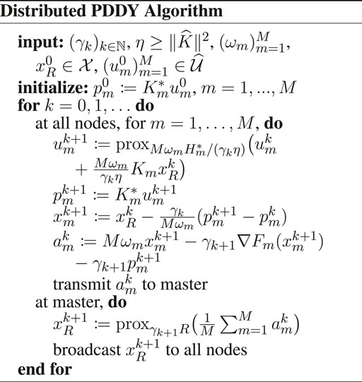
6.2 The Distributed PDDY Algorithm

The Distributed PDDY Algorithm, shown above, is derived the same way as the Distributed PD3O Algorithm. However, the smoothness constant cannot be defined only on $\mathcal{S}$, so that we have

$L_{\widehat{F}}={\max }_{m=1,\dots ,M}\frac{L_{F_m}}{M{\omega }_m}$

and

${\mu }_{\widehat{F}}={\min }_{m=1,\dots ,M}\frac{{\mu }_{F_m}}{M{\omega }_m}.$

Moreover,

$\Vert \widehat{K}{\Vert }^2={\max }_{m=1,\dots ,M}\Vert K_m{\Vert }^2,(23)$

except if F_m ≡ 0, in which case the Distributed PDDY Algorithm becomes the Distributed Chambolle–Pock Algorithm Form II, for which we can set

$\Vert \widehat{K}{\Vert }^2=\Vert \sum _{m=1}^M{\omega }_m{K}_m*K_m\Vert .(24)$

We can note that when K_m ≡ I, the Distributed PDDY Algorithm reverts to a form of distributed Davis–Yin algorithm, which is different from the Distributed Davis–Yin Algorithm obtained from the PD3O algorithm, shown above. Similarly, when R = 0, we obtain a different algorithm than the Distributed Loris–Verhoeven Algorithm shown above. When F_m ≡ 0, the Distributed PDDY Algorithm reverts to the Distributed Chambolle–Pock Algorithm Form II, which is still different from the Distributed Douglas–Rachford Algorithm when K_m ≡ I.

The counterpart of Theorem 2 is:

Theorem 9. (convergence of the Distributed PDDY Algorithm). In the Distributed PDDY Algorithm, suppose that γ_k ≡ γ ∈ (0, 2/L_F) and $\eta \ge \Vert \widehat{K}{\Vert }^2$, where $\Vert \widehat{K}{\Vert }^2$ is defined in (23) or (24). Then all $x_m^k$ as well as $x_R^k$ converge to the same solution x^* of (1), and every $u_m^k$ converges to some element $u_m^{*}$.The counterpart of Theorem 4 is:

Theorem 10. (Accelerated Distributed PDDY Algorithm). Suppose that ${\mu }_{\widehat{F}}>0$. Let x^* be the unique solution to (1). Let κ ∈ (0, 1) and ${\gamma }_0\in (\mathrm{0,2}(1-\kappa )/L_{\widehat{F}})$. Set γ₁ = γ₀ and

${\gamma }_{k+1}=-{\gamma }_k^2{\mu }_{\widehat{F}}\kappa +{\gamma }_k\sqrt{{({\gamma }_k{\mu }_{\widehat{F}}\kappa )}^2+1},\text{for\hspace{0.17em}every\hspace{0.17em}}k\ge 1.$

Suppose that $\eta \ge \Vert \widehat{K}{\Vert }^2$, where $\Vert \widehat{K}{\Vert }^2$ is defined in (23) or (24). Then in the Distributed PDDY Algorithm, there exists ${\widehat{c}}_0>0$ such that, for every k ≥ 1,

$\sum _{m=1}^M{\omega }_m\Vert x_m^{k+1}-x*{\Vert }^2\le \frac{{\gamma }_{k+1}^2}{1-{\gamma }_{k+1}{\mu }_F\kappa }{c}_0=O\left(1/k^2\right).$

Consequently, for every m = 1, … , M,

$\Vert x_m^k-x*{\Vert }^2=O\left(1/k^2\right).$

Moreover, if $\eta >\Vert \widehat{K}{\Vert }^2$, $\Vert x_R^k-x*{\Vert }^2=O(1/k^2)$ as well.The counterpart of Theorem 5 is:

Theorem 11. (linear convergence of the Distributed PDDY Algorithm). Suppose that ${\mu }_{\widehat{F}}+{\mu }_R>0$ and that every H_m is L_m-smooth, for some L_m > 0. Let x^* be the unique solution to (1). Suppose that ${\gamma }_k\equiv \gamma \in (\mathrm{0,2}/L_{\widehat{F}})$ and $\eta \ge \Vert \widehat{K}{\Vert }^2$, where $\Vert \widehat{K}{\Vert }^2$ is defined in (23) or (24). Then the Distributed PDDY Algorithm converges linearly: there exists ρ ∈ (0, 1] and ${\widehat{c}}_0>0$ such that, for every $k\in \mathbb{N}$,

$\Vert x_R^{k+1}-x^{*}{\Vert }^2\le {(1-\rho )}^k{\widehat{c}}_0.$

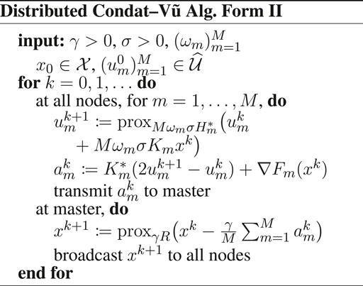
6.3 The Distributed Condat–Vũ Algorithm

We can apply our product-space technique to other algorithms; in particular, we can derive distributed versions, shown below, of the Condat–Vũ algorithm (Condat, 2013; Vũ, 2013; Condat et al., 2019a), which is a well known algorithm for the problem (Eq. 2).

The smoothness constant $L_{\widehat{F}}^2$ is the same as for the Distributed PD3O Algorithm; we can set $L_{\widehat{F}}^2=\frac{1}{M^2}{\sum }_{m=1}^M{L}_{F_m}^2/{\omega }_m$.

Moreover, the norm of $\widehat{K}$ is smaller for the Condat–Vũ algorithm: we have $\Vert \widehat{K}{\Vert }^2=\Vert {\sum }_{m=1}^M{\omega }_m{K}_m^{*}{K}_m\Vert$, whatever the functions F_m. This is because the gradient descent step is completely decoupled from the dual variables in the Condat–Vũ algorithm.

The price to pay is a stronger condition on the parameters for convergence:

Theorem 12. (convergence of the Distributed Condat–Vũ Algorithm). Suppose that the parameters γ > 0 and σ > 0 are such that

$\gamma \left(\sigma \Vert \sum _{m=1}^M{\omega }_m{K}_m^{*}{K}_m\Vert +\frac{L_{\widehat{F}}}{2}\right)<1.$

Then x^k converges to a solution x^* of (1). Also, $u_m^k$ converges to some element $u_m^{*}\in {\mathcal{U}}_m$, for every m = 1, … , M.When F_m ≡ 0, the two forms of the Distributed Condat–Vũ Algorithm revert to the two forms of the Distributed Chambolle–Pock Algorithm, respectively. In that case, with constant stepsizes γ_k ≡ γ, the convergence condition is $\gamma \sigma \Vert {\sum }_{m=1}^M{\omega }_m{K}_m^{*}{K}_m\Vert \le 1$, which is the same as above with σ = 1/(ηγ).

Data Availability Statement

Publicly available datasets were analyzed in this study. This data can be found here: LibSVM, https://www.csie.ntu.edu.tw/∼cjlin/libsvm/.

Author Contributions

GM wrote the code and generated the results for the SVM experiment in Section 4.3. PR contributed to the paper writing and to the project management. LC did all the rest.

Conflict of Interest

The authors declare that the research was conducted in the absence of any commercial or financial relationships that could be construed as a potential conflict of interest.

Publisher’s Note

All claims expressed in this article are solely those of the authors and do not necessarily represent those of their affiliated organizations, or those of the publisher, the editors and the reviewers. Any product that may be evaluated in this article, or claim that may be made by its manufacturer, is not guaranteed or endorsed by the publisher.

References

Alghunaim, S. A., Ryu, E. K., Yuan, K., and Sayed, A. H. (2021). Decentralized Proximal Gradient Algorithms with Linear Convergence Rates. IEEE Trans. Automat. Contr. 66, 2787–2794. doi:10.1109/tac.2020.3009363

CrossRef Full Text | Google Scholar

Bach, F., Jenatton, R., Mairal, J., and Obozinski, G. (2012). Optimization with Sparsity-Inducing Penalties. Found. Trends Mach. Learn. 4, 1–106. doi:10.1561/2200000015

CrossRef Full Text | Google Scholar

Bauschke, H. H., and Combettes, P. L. (2017). Convex Analysis and Monotone Operator Theory in Hilbert Spaces. 2nd edn. New York: Springer.

Google Scholar

Beck, A. (2017). “First-Order Methods in Optimization,” in MOS-SIAM Series on Optimization (SIAM).

Google Scholar

Boţ, R. I., Csetnek, E. R., and Hendrich, C. (2014). “Recent Developments on Primal–Dual Splitting Methods with Applications to Convex Minimization,” in Mathematics without Boundaries: Surveys in Interdisciplinary Research. Editors P. M. Pardalos, and T. M. Rassias (New York: Springer), 57–99.

Google Scholar

Bredies, K., Kunisch, K., and Pock, T. (2010). Total Generalized Variation. SIAM J. Imaging Sci. 3, 492–526. doi:10.1137/090769521

CrossRef Full Text | Google Scholar

Bubeck, S. (2015). Convex Optimization: Algorithms and Complexity. FNT Machine Learn. 8, 231–357. doi:10.1561/2200000050

CrossRef Full Text | Google Scholar

Cevher, V., Becker, S., and Schmidt, M. (2014). Convex Optimization for Big Data: Scalable, Randomized, and Parallel Algorithms for Big Data Analytics. IEEE Signal. Process. Mag. 31, 32–43. doi:10.1109/msp.2014.2329397

CrossRef Full Text | Google Scholar

Chambolle, A., and Pock, T. (2011). A First-Order Primal-Dual Algorithm for Convex Problems with Applications to Imaging. J. Math. Imaging Vis. 40, 120–145. doi:10.1007/s10851-010-0251-1

CrossRef Full Text | Google Scholar

Chambolle, A., and Pock, T. (2016a). An Introduction to Continuous Optimization for Imaging. Acta Numerica 25, 161–319. doi:10.1017/s096249291600009x

CrossRef Full Text | Google Scholar

Chambolle, A., and Pock, T. (2016b). On the Ergodic Convergence Rates of a First-Order Primal-Dual Algorithm. Math. Program 159, 253–287. doi:10.1007/s10107-015-0957-3

CrossRef Full Text | Google Scholar

Chang, C.-C., and Lin, C.-J. (2011). LibSVM: A Library for Support Vector Machines. ACM Trans. Intell. Syst. Technol. 2, 27. doi:10.1145/1961189.1961199

CrossRef Full Text | Google Scholar

Chen, P., Huang, J., and Zhang, X. (2013). A Primal–Dual Fixed point Algorithm for Convex Separable Minimization with Applications to Image Restoration. Inverse Probl. 29, 025011. doi:10.1088/0266-5611/29/2/025011

CrossRef Full Text | Google Scholar

Combettes, P. L., Condat, L., Pesquet, J.-C., and Vũ, B. C. (2014). “A Forward–Backward View of Some Primal–Dual Optimization Methods in Image Recovery,” in Proc. Of IEEE ICIP (Paris, France: IEEE), 4141–4145.

Google Scholar

Combettes, P. L., and Pesquet, J.-C. (2012). Primal-Dual Splitting Algorithm for Solving Inclusions with Mixtures of Composite, Lipschitzian, and Parallel-Sum Type Monotone Operators. Set-valued Anal. 20, 307–330. doi:10.1007/s11228-011-0191-y

CrossRef Full Text | Google Scholar

Combettes, P. L., and Pesquet, J.-C. (2010). “Proximal Splitting Methods in Signal Processing,” in Fixed-Point Algorithms for Inverse Problems in Science and Engineering. Editors H. H. Bauschke, R. Burachik, P. L. Combettes, V. Elser, D. R. Luke, and H. Wolkowicz (New York: Springer-Verlag), 185–212.

Google Scholar

Condat, L. (2017a). “A Convex Approach to K-Means Clustering and Image Segmentation,” in Proc. Of EMMCVPR. Lecture Notes in Computer Science. Editors M. Pelillo, and E. Hancock (Venice, Italy: Springer, 2018), Vol. 10746, 220–234.

Google Scholar

Condat, L. (2014). A Generic Proximal Algorithm for Convex Optimization—Application to Total Variation Minimization. IEEE Signal. Process. Lett. 21(8), 985–989. doi:10.1109/LSP.2014.2322123

CrossRef Full Text | Google Scholar

Condat, L. (2013). A Primal-Dual Splitting Method for Convex Optimization Involving Lipschitzian, Proximable and Linear Composite Terms. J. Optim. Theor. Appl. 158, 460–479. doi:10.1007/s10957-012-0245-9

CrossRef Full Text | Google Scholar

Condat, L. (2017b). Discrete Total Variation: New Definition and Minimization. SIAM J. Imaging Sci. 10, 1258–1290. doi:10.1137/16m1075247

CrossRef Full Text | Google Scholar

Condat, L., Kitahara, D., Contreras, A., and Hirabayashi, A. (2019a). Proximal Splitting Algorithms: A Tour of Recent Advances, with New Twists. Preprint arXiv:1912.00137.

Google Scholar

Condat, L., Kitahara, D., and Hirabayashi, A. (2019b). “A Convex Lifting Approach to Image Phase Unwrapping,” in Proc. Of IEEE ICASSP (Brighton, UK: IEEE), 1852–1856. doi:10.1109/icassp.2019.8682258

CrossRef Full Text | Google Scholar

Cremers, D., Pock, T., Kolev, K., and Chambolle, A. (2011). “Convex Relaxation Techniques for Segmentation, Stereo and Multiview Reconstruction,” in Markov Random Fields for Vision and Image Processing (Cambridge: MIT Press).

Google Scholar

Davis, D., and Yin, W. (2017). A Three-Operator Splitting Scheme and its Optimization Applications. Set-valued Anal. 25, 829–858. doi:10.1007/s11228-017-0421-z

CrossRef Full Text | Google Scholar

Drori, Y., Sabach, S., and Teboulle, M. (2015). A Simple Algorithm for a Class of Nonsmooth Convex-Concave Saddle-point Problems. Operations Res. Lett. 43, 209–214. doi:10.1016/j.orl.2015.02.001

CrossRef Full Text | Google Scholar

Duran, J., Moeller, M., Sbert, C., and Cremers, D. (2016). Collaborative Total Variation: A General Framework for Vectorial TV Models. SIAM J. Imaging Sci. 9, 116–151. doi:10.1137/15m102873x

CrossRef Full Text | Google Scholar

Gorbunov, E., Hanzely, F., and Richtárik, P. (2020). A Unified Theory of SGD: Variance Reduction, Sampling, Quantization and Coordinate Descent. Proc. Int. Conf. Artif. Intell. Stat. (Aistats), PMLR 108, 680–690.

Google Scholar

Komodakis, N., and Pesquet, J.-C. (2015). Playing with Duality: An Overview of Recent Primal?dual Approaches for Solving Large-Scale Optimization Problems. IEEE Signal. Process. Mag. 32, 31–54. doi:10.1109/msp.2014.2377273

CrossRef Full Text | Google Scholar

Konečný, J., McMahan, H. B., Yu, F. X., Richtárik, P., Suresh, A. T., and Bacon, D. (2016). “Federated Learning: Strategies for Improving Communication Efficiency,” NIPS Private Multi-Party Machine Learn. Workshop. Paper arXiv:1610.05492.

Google Scholar

Latafat, P., Freris, N. M., and Patrinos, P. (2019). A New Randomized Block-Coordinate Primal-Dual Proximal Algorithm for Distributed Optimization. IEEE Trans. Automat. Contr. 64, 4050–4065. doi:10.1109/tac.2019.2906924

CrossRef Full Text | Google Scholar

Loris, I., and Verhoeven, C. (2011). On a Generalization of the Iterative Soft-Thresholding Algorithm for the Case of Non-separable Penalty. Inverse Probl. 27, 125007. doi:10.1088/0266-5611/27/12/125007

CrossRef Full Text | Google Scholar

Malinovsky, G., Kovalev, D., Gasanov, E., Condat, L., and Richtárik, P. (2020). “From Local SGD to Local Fixed point Methods for Federated Learning,” in Proceedings of the 37th International Conference on Machine Learning, PMLR, 119, 6692–6701.

Google Scholar

O’Connor, D., and Vandenberghe, L. (2020). On the Equivalence of the Primal-Dual Hybrid Gradient Method and Douglas–Rachford Splitting. Math. Program 179, 85–108. doi:10.1007/s10107-018-1321-1

CrossRef Full Text | Google Scholar

Palomar D. P., and Eldar Y. C. (Editors) (2009). Convex Optimization in Signal Processing and Communications (Cambridge: Cambridge University Press).

Google Scholar

Parikh, N., and Boyd, S. (2014). Proximal Algorithms. FNT in Optimization 1, 127–239. doi:10.1561/2400000003

CrossRef Full Text | Google Scholar

Polson, N. G., Scott, J. G., and Willard, B. T. (2015). Proximal Algorithms in Statistics and Machine Learning. Statist. Sci. 30, 559–581. doi:10.1214/15-sts530

CrossRef Full Text | Google Scholar

Glowinski R., Osher S. J., and Yin W. (Editors) (2016). Splitting Methods in Communication, Imaging, Science, and Engineering (New York: Springer International Publishing).

Google Scholar

Richtárik, P., and Takáč, M. (2014). Iteration Complexity of Randomized Block-Coordinate Descent Methods for Minimizing a Composite Function. Math. Program 144, 1–38. doi:10.1007/s10107-012-0614-z

CrossRef Full Text | Google Scholar

Ryu, E. K., and Yin, W. (2017). Proximal-proximal-gradient Method. Preprint arXiv:1708.06908.

Google Scholar

Salim, A., Condat, L., Kovalev, D., and Richtárik, P. (2021). An Optimal Algorithm for Strongly Convex Minimization under Affine Constraints. Preprint arXiv:2102.11079.

Google Scholar

Salim, A., Condat, L., Mishchenko, K., and Richtárik, P. (2020). Dualize, Split, Randomize: Fast Nonsmooth Optimization Algorithms. Preprint arXiv:2004.02635.

Google Scholar

Scaman, K., Bach, F., Bubeck, S., Lee, Y. T., and Massoulié, L. (2017). Optimal Algorithms for Smooth and Strongly Convex Distributed Optimization in Networks. Proc. 34th Int. Conf. Machine Learn. (Icml) 70, 3027–3036.

Google Scholar

Shi, W., Ling, Q., Wu, G., and Yin, W. (2015). EXTRA: An Exact First-Order Algorithm for Decentralized Consensus Optimization. SIAM J. Optim. 25, 944–966. doi:10.1137/14096668x

CrossRef Full Text | Google Scholar

Sra, S., Nowozin, S., and Wright, S. J. (2011). Optimization for Machine Learning. Cambridge: The MIT Press.

Google Scholar

Stathopoulos, G., Shukla, H., Szucs, A., Pu, Y., and Jones, C. N. (2016). Sensor Fault Diagnosis. FnT Syst. Control. 3, 249–362. doi:10.1561/2600000008

CrossRef Full Text | Google Scholar

Unknown author (1972). Every Convex Function Is Locally Lipschitz. The Am. Math. Monthly 79, 1121–1124.

Google Scholar

Vũ, B. C. (2013). A Splitting Algorithm for Dual Monotone Inclusions Involving Cocoercive Operators. Adv. Comput. Math. 38, 667–681. doi:10.1007/s10444-011-9254-8

CrossRef Full Text | Google Scholar

Wang, Y.-X., Sharpnack, J., Smola, A., and Tibshirani, R. (2016). Trend Filtering on Graphs. J. Machine Learn. Res. 17, 1–41.

Google Scholar

Yan, M. (2018). A New Primal-Dual Algorithm for Minimizing the Sum of Three Functions with a Linear Operator. J. Sci. Comput. 76, 1698–1717. doi:10.1007/s10915-018-0680-3

CrossRef Full Text | Google Scholar