Multivariate Lipschitz Analysis of the Stability of Neural Networks

1 Introduction

Artificial neural networks are at the core of recent advances in Artificial Intelligence. One of the main challenges faced today, especially by companies designing advanced industrial systems, is to ensure the safety of new generations of products using these technologies. Neural networks have been shown to be sensitive to adversarial perturbations (Szegedy et al., 2013). For example, changing a few pixels of an image may lead to misclassification of the image by a Deep Neural Network (DNN), which emphasizes the potential lack of stability of such architectures. DNNs being sensitive to adversarial examples, can thus be fooled, in an intentional manner (security issue) or in undeliberate/accidental manner (safety issue), which raises a major stability concern for safety-critical systems which need to be certified by an independent certification authority prior to any entry into production/operation. DNN-based solutions are hindered with such issue due to their complex nonlinear structure. Attempts towards verification of neural networks have been made for example in (Katz et al., 2017; Weng et al., 2019). It has been proven in (Tsipras et al., 2018b) that there exists a trade-off between the prediction performance and the stability of neural networks.

In the last years, the number of works devoted to the stability issue of neural networks has grown in manifolds. In these works, the terms “stability”, “robustness” or “local robustness” are used interchangeably with the same meaning which is formally defined in this paper as the extent to which a neural network can continue to operate correctly despite small perturbations in its inputs. The stability criterion considered here highlights the fact that these small perturbations in the inputs do not produce high variations of the outputs. Many approaches have been proposed, some dedicated to specific architectures (e.g., networks using only ReLU activation functions) and grounded on more or less empirical techniques. We can break down broadly these techniques into three categories:

• Purely computational approaches which consist in attacking a neural network and observing its response to such attacks,

• methods based on (often clever) heuristics for testing/promoting the stability of a neural net,

• studies that aim at establishing mathematical proofs of stability.

These three kinds of strategies are useful for building and certifying effectively robust neural networks. However, the techniques based on mathematical proofs of stability are generally preferred by industrial safety experts since they enable a safe-by-design approach that is more efficient than a robustness verification activity done a posteriori with a necessarily bounded effort. Among the possible mathematical approaches, we focus in this article on those relying upon the analysis of the Lipschitz properties of neural networks. Such properties play a fundamental role in the understanding of the internal mechanisms governing these complex nonlinear systems. Besides, they make few assumptions on the type of non-linearities used and are thus valid for a wide range of networks. Nevertheless, they generate a number of challenges both from a theoretical and numerical standpoints.

Since DNNs are sensitive to small specific perturbations, providing a quantitative estimation of the stability of such architectures is of paramount importance for safe and secure product development in domains such as aeronautics, ground transportation, autonomous vehicles, energy, and healthcare. One metric to assess the stability of neural networks to adversarial perturbations is the Lipschitz constant, which upper bounds the ratio between output variations and input variations for a given metric. More generally, in deep learning theory, novel generalization bounds critically rely on the Lipschitz constant of the neural network (Bartlett et al., 2017). One of the main limitations of the Lipschitz constant, defined in either global or local context, is that it only provides a single parameter to quantify the robustness of a neural network. Such a single-parameter analysis does not facilitate the understanding of potential sources of instability. In particular, it may be insightful to identify the inputs which have the highest impact in terms of sensitivity. In the context of tabular data mining, the inputs often have quite heterogeneous characteristics. Some of them are categorical data, often encoded in a specific way [e.g., one-hot encoder (Hancock and Khoshgoftaar, 2020)] and among them, one can usually distinguish those which are unsorted (like labels identifying countries) or those which are sorted (like severity scores in a disease). So, it may appear useful to analyze in a specific manner each type of inputs of a NN and even sometimes to exclude some of these inputs (e.g., unsorted categorical data for which the notion of small perturbation may be meaningless) from the performed sensitivity analysis.

The contributions of the work are summarized below:

• A multivariate analysis of the Lipschitz properties of NNs is performed by generating a set of partial Lipschitz constants. This opens a new dimension to studying the stability of NNs.

• Our sensitivity analysis allows us to capture the behaviour of an individual input or group of inputs.

• The results of this analysis are displayed by a new graphical representation termed as a Lipschitz star.

• Using the proposed analysis, we also study quantitatively the effect of spectral normalization constraint and adversarial training on the stability of NNs.

• We showcase our results on various open-source datasets along with a real industrial application in the domain of Air Traffic Management.

In the next section we give a detailed description of the state-of-the-art related to the quantification of the Lipschitz constant in neural networks. Section 3 gives our proposed method pertaining to sensitivity of inputs and introduction to Lipschitz stars. Section 4 provides an analytical evaluation for our approach with synthetic datasets. The next section gives detailed results on three open source datasets and a real safety critical industrial dataset. The last section concludes our paper.

2 Overview on the Estimation of the Lipschitz Constant of Feedforward Networks

2.1 Theoretical Background

An m-layered feedforward network can be modelled by the following recursive equations:

$\left(\forall i\in \left\{1,\dots ,m\right\}\right)x_i=T_i\left(x_{i-1}\right)=R_i\left(W_i{x}_{i-1}+b_i\right),(1)$

where, at the ith layer, $x_{i-1}\in {\mathbb{R}}^{N_{i-1}}$ designates the input vector, $x_i\in {\mathbb{R}}^{N_i}$ the output one, $W_i\in {\mathbb{R}}^{N_i\times N_{i-1}}$ is the weight matrix, $b_i\in {\mathbb{R}}^{N_i}$ is the bias vector, and $R_i:{\mathbb{R}}^{N_i}\to {\mathbb{R}}^{N_i}$ is the activation operator. This operator may consist of the application of basic nonlinear functions, e.g., ReLU or tanh, to each component of the input. Alternatively, it may consist of a softmax operation or group sorting operations which typically arise in max pooling. In this model, when the matrix W_i has a Toeplitz or a block-Toeplitz structure, a convolutive layer is obtained.

Since the seminal work in (Szegedy et al., 2013), it is known that instability in the outputs of the neural networks may arise. This issue, often referred to as the stability with respect to adversarial noise, tends to be more severe when the training set is small. However, it may even happen with large datasets such as ImageNet. As shown in (Goodfellow et al., 2015), the problem is mainly related to the choice of the weight matrices. One way of quantifying the stability of the system is to calculate a Lipschitz constant of the network.

A Lipschitz constant of a function T is an upper bound on the ratio between the variations of the output values and the variations of input arguments of a function T. Thus, it is a measure of sensitivity of the function with respect to input perturbations. This means that, if $\theta \in \left[0,+\right.\infty \left[\right.$ is such that, for every input $x\in {\mathbb{R}}^{N_0}$ and perturbation $z\in {\mathbb{R}}^{N_0}$,

$\Vert T\left(x+z\right)-T\left(x\right)\Vert \le \theta \Vert z\Vert ,(2)$

then θ is a Lipschitz constant of T. Note that, the same notation is used here for the norms on ${\mathbb{R}}^{N_0}$ and ${\mathbb{R}}^{N_m}$, but actually different norms can be used. If not specified, the standard Euclidean norm will be used. Another important remark which follows from the mean value inequality is that, if T is differentiable on ${\mathbb{R}}^{N_0}$, the optimal (i.e., smallest) Lipschitz constant is

$\theta ={\sup }_{x\in {\mathbb{R}}^{N_0}}\Vert T^{\prime }\left(x\right){\Vert }_{\text{S}}={\sup }_{x\in {\mathbb{R}}^{N_0}}{\sup }_{x\in {\mathbb{R}}^{N_0}}\frac{\Vert T^{\prime }\left(x\right)z\Vert }{\Vert z\Vert },(3)$

where $T^{\prime }(x)\in {\mathbb{R}}^{N_m\times N_0}$ is the Jacobian matrix of T at x and ‖ ⋅‖_S denotes the spectral matrix norm. Local definitions of the Lipschitz constant are also possible (Yang et al., 2020). In order to get more meaningful expressions of Lipschitz constants, an important assumption which will be made in this paper is that the operators ${(R_i)}_{1\le i\le m}$ are nonexpansive, i.e., 1-Lipschitz. This assumption is satisfied for all the standard choices of activation operators.

The first upper-bound on the Lipschitz constant of a neural network was derived by analyzing the effect of each layer independently and considering a product of the resulting spectral norms (Goodfellow et al., 2015). This leads to the following Trivial Upper Bound:

${\bar{\theta }}_m=\Vert W_m{\Vert }_{\text{S}}\Vert W_{m-1}{\Vert }_{\text{S}}\dots ,\Vert W_1{\Vert }_{\text{S}}.(4)$

Although easy to compute, this upper bound turns out be over-pessimistic. In (Virmaux and Scaman, 2018), the problem of computing the exact Lipschitz constant of a differentiable function is pointed out to be NP-hard. A first generic algorithm (AutoLip) for upper bounding the Lipschitz constant of any differentiable function is proposed. This bound however reduces to Eq. 4 for standard feedforward neural networks. Additionally, the authors proposed an algorithm, called SeqLip, for sequential neural networks, which shows significant improvement over AutoLip. A sequential neural network is a network for which the activation operators are separable in the sense that, for every i ∈ (1, … , m),

$\left(\forall x_i={\left({\xi }_{i,k}\right)}_{1\le k\le N_i}\in {\mathbb{R}}^{N_i}\right)R_i\left(x\right)={\left({\rho }_i\left({\xi }_{i,k}\right)\right)}_{1\le k\le N_i},(5)$

where the activation function ${\rho }_i:\mathbb{R}\to \mathbb{R}$¹. In (Virmaux and Scaman, 2018), it is assumed that the functions ${({\rho }_i)}_{1\le i\le m}$ are differentiable, increasing, and their derivative are upper bounded by one. It can be deduced that a Lipschitz constant of the network is

${\vartheta }_m={\sup }_{{\mathrm{\Lambda }}_1\in {\mathcal{D}}_{N_1}\left(\left[\mathrm{0,1}\right]\right),\dots ,{\mathrm{\Lambda }}_{m-1}\in {\mathcal{D}}_{N_{m-1}}\left(\left[\mathrm{0,1}\right]\right)}\Vert W_m{\mathrm{\Lambda }}_{m-1}\dots ,{\mathrm{\Lambda }}_1{W}_1{\Vert }_{\text{S}},(6)$

where ${\mathcal{D}}_N(I)$ designates the set of diagonal matrices of dimension N × N with diagonal values in $I\subset \mathbb{R}$. This bound simplifies as

${\vartheta }_m={\sup }_{{\mathrm{\Lambda }}_1\in {\mathcal{D}}_{N_1}\left(\left\{\mathrm{0,1}\right\}\right),\dots ,{\mathrm{\Lambda }}_{m-1}\in {\mathcal{D}}_{N_{m-1}}\left(\left\{\mathrm{0,1}\right\}\right)}\Vert W_m{\mathrm{\Lambda }}_{m-1}\dots ,{\mathrm{\Lambda }}_1{W}_1{\Vert }_{\text{S}},(7)$

which shows that $2^{N_i}$ values of the diagonal elements of matrix Λ_i have to be tested at each layer i ∈ (1, … , m), so that the global complexity amounts to $2^{N_1+\cdots +N_{m-1}}$ and thus grows exponentially as a function of the number of neurons. Estimating the Lipschitz constant using this method is intractable even for medium-size networks; thus, the authors use a greedy algorithm to compute a bound, which may under-approximate the Lipschitz constant. This does not provide true upper bounds.

In Combettes and Pesquet (2020b) various bounds on the Lipschitz constant of a feedforward network are derived by assuming that, for every i ∈ (1, … , m) the activation operator R_i is α_i-averaged with $\left.{\alpha }_i\in \right]\left.\mathrm{0,1}\right]$. We recall that this means that there exists a non-expansive (i.e., 1-Lipschitz) operator Q_i such that R_i = (1−α_i)Id + α_iQ_i. The following inequality is then satisfied:

$\left(\forall \left(x,y\right)\in {\mathbb{R}}^{N_i}\right)\Vert R_i\left(x\right)-R_i\left(y\right){\Vert }^2\le \Vert x-y{\Vert }^2-\frac{1-{\alpha }_i}{{\alpha }_i}\Vert x-R_i\left(x\right)-y+R_i\left(y\right){\Vert }^2.(8)$

We thus see that the smaller α_i, the more “stable” R_i is. In the limit case when α₁ = 1, R_i is non-expansive and, when α_i = 1/2, R_i is said to be firmly nonexpansive. An important subclass of firmly nonexpansive operators is the class of proximity operators of convex functions which are proper and lower-semicontinuous. Let ${\mathrm{\Gamma }}_0({\mathbb{R}}^N)$ be the class of such functions defined from ${\mathbb{R}}^N$ to $\left]-\infty ,+\infty \right]$. The proximity operator of a function $f\in {\mathrm{\Gamma }}_0({\mathbb{R}}^N)$, at some point $x\in {\mathbb{R}}^N$, is the unique vector denoted by prox_f(x) such that

${\text{prox}}_f\left(x\right)=\underset{p\in {\mathbb{R}}^N}{\text{argmin}}\frac{1}{2}\Vert p-x{\Vert }^2+f\left(p\right).(9)$

The proximity operator is a fundamental tool in convex optimization. As shown in (Combettes and Pesquet, 2020a), the point is that most of the activation functions (e.g., sigmoid, ReLu, leaky ReLU, ELU) currently used in neural networks are the proximity operators of some proper lower-semicontinuous convex functions. This property is also satisfied by activation operators which are not separable, like softmax or the squashing function used in capsule networks. The few activation operators which are not proximity operators (e.g., convex combinations of a max pooling and an average pooling) can be viewed as over-relaxations of proximity operators and correspond to a value of the averaging parameter greater than 1/2.

Based on these averaging assumptions, a first estimation of the Lipschitz constant is given by

${\theta }_m={\beta }_{m;\varnothing }\Vert W_m◦\dots ,◦W_1\Vert +\sum _{k=1}^{m-1}\sum _{\left(j_1,\dots ,j_k\right)\in {\mathbb{J}}_{m,k}}{\beta }_{m;\left\{j_1,\dots ,j_k\right\}}{\sigma }_{m;\left\{j_1,\dots ,j_k\right\}},(10)$

where

$\left(\forall \mathbb{J}\subset \left\{1,\dots ,m-1\right\}\right){\beta }_{m;\mathbb{J}}=\left(\prod _{j\in \mathbb{J}}{\alpha }_j\right)\prod _{j\in \left\{1,\dots ,m-1\right\}\backslash \mathbb{J}}\left(1-{\alpha }_j\right),(11)$

for every k ∈ (1, … , m−1),

${\mathbb{J}}_{m,k}=\left\{\begin{array}{cc}\left\{\left(j_1,\dots ,j_k\right)\in {\mathbb{N}}^k\left|\right.1\le j_1<\dots ,<j_k\le m-1\right\},\hfill & \text{if}k>1;\hfill \\ \left\{1,\dots ,m-1\right\},\hfill & \text{if}k=1\hfill \end{array}\right.(12)$

and for every $(j_1,\dots ,j_k)\in {\mathbb{J}}_{m,k}$,

${\sigma }_{m;\left\{j_1,\dots ,j_k\right\}}=\Vert W_m\dots ,W_{j_k+1}{\Vert }_{\text{S}}\Vert W_{j_k}\dots ,W_{j_{k-1}+1}{\Vert }_{\text{S}}\dots \Vert W_{j_1}\dots ,W_1{\Vert }_{\text{S}}(13)$

When, for every i ∈ (1, … , m−1), R_i is firmly nonexpansive, the expression simplifies as

${\theta }_m=\frac{1}{2^{m-1}}\left(\Vert W_m\dots ,W_1{\Vert }_{\text{S}}+\sum _{k=1}^{m-1}\sum _{\left(j_1,\dots ,j_k\right)\in {\mathbb{J}}_{m,k}}{\sigma }_{m;\left\{j_1,\dots ,j_k\right\}}\right)(14)$

If, for every i ∈ (1, … , m−1), R_i is separable², a second estimation is provided which reads

${\vartheta }_m={\sup }_{\begin{array}{c}{\mathrm{\Lambda }}_1\in {\mathcal{D}}_{N_1}\left(\left\{2{\alpha }_1-\mathrm{1,1}\right\}\right),\\ ⋮,\\ {\mathrm{\Lambda }}_{m-1}\in {\mathcal{D}}_{N_{m-1}}\left(\left\{2{\alpha }_{m-1}-\mathrm{1,1}\right\}\right)\end{array}}\Vert W_m{\mathrm{\Lambda }}_{m-1}\dots ,{\mathrm{\Lambda }}_1{W}_1{\Vert }_{\text{S}}(15)$

We thus see that, when α₁ = … = α_m−1 = 1/2, we recover Eq. 7 without making any assumption on the differentiability of the activation functions. This estimation is more accurate than the previous one in the sense that

$\Vert W_m\dots ,W_1{\Vert }_{\text{S}}\le {\vartheta }_m\le {\theta }_m.(16)$

It is proved in (Combettes and Pesquet, 2020b) that, if the network is with non-negative weights, that is $(\forall i\in \{1,\dots ,m\})W_i\in \left[0,+\infty \right.{\left[\right.}^{N_i\times N_i}$, the lower bound in Eq. 16 is attained, i.e.,

${\vartheta }_m=\Vert W_m\dots ,W_1{\Vert }_{\text{S}}.(17)$

Another interesting result which is established in (Combettes and Pesquet, 2020b) is that similar results hold if other norms than the Euclidean norm are used to quantify the perturbations on the input and the output. For example, for a given i ∈ (1, … , m), for every p ∈ (1, + ∞), we can define the following norm:

$\left(\forall x_i={\left({\xi }_{i,k}\right)}_{1\le k\le N_i}\in {\mathbb{R}}^{N_i}\right)\Vert x{\Vert }_p=\left\{\begin{array}{cc}\left|\right.\sum _{k=1}^{N_i}|{\xi }_{i,k}{|}^p{\left|\right.}^{1/p},\hfill & \text{if}p<+\infty \hfill \\ {\sup }_{1\le k\le N_i}|{\xi }_{i,k}|,\hfill & \text{if}p=+\infty .\hfill \end{array}\right.(18)$

If (p, q) ∈ (1,+∞)², the input space ${\mathbb{R}}^{N_0}$ is equipped with the norm ‖ ⋅‖_p, and the output space ${\mathbb{R}}^{N_m}$ is equipped with the norm ‖ ⋅‖_q, a Lipschitz constant for a network with separable activation operators is

${\vartheta }_m={\sup }_{\begin{array}{c}{\mathrm{\Lambda }}_1\in {\mathcal{D}}_{N_1}\left(\left[2{\alpha }_1-\mathrm{1,1}\right]\right),\\ ⋮,\\ {\mathrm{\Lambda }}_{m-1}\in {\mathcal{D}}_{N_{m-1}}\left(\left[2{\alpha }_{m-1}-\mathrm{1,1}\right]\right)\end{array}}\Vert W_m{\mathrm{\Lambda }}_{m-1}\dots ,{\mathrm{\Lambda }}_1{W}_1{\Vert }_{p,q}(19)$

$={\sup }_{\begin{array}{c}{\mathrm{\Lambda }}_1\in {\mathcal{D}}_{N_1}\left(\left\{2{\alpha }_1-\mathrm{1,1}\right\}\right),\\ ⋮,\\ {\mathrm{\Lambda }}_{m-1}\in {\mathcal{D}}_{N_{m-1}}\left(\left\{2{\alpha }_{m-1}-\mathrm{1,1}\right\}\right)\end{array}}\Vert W_m{\mathrm{\Lambda }}_{m-1}\dots ,{\mathrm{\Lambda }}_1{W}_1{\Vert }_{p,q}(20)$

where ‖ ⋅‖_p,q is the subordinate L_p,q matrix norm induced by the two previous norms. The ability to use norms other than the Euclidean one may be sometimes more meaningful in practice (especially for the ℓ₁ or the sup norm). However, computing such a subordinate norm is not always easy (Lewis, 2010).

2.2 SDP-Based Approach

The work in (Fazlyab et al., 2019) focuses on neural networks using separable activation operators. It assumes that the activation function ρ_i used at a layer i ∈ (1, … , m) is slope-bounded, i.e., there exist nonnegative parameters ϒ_min and ϒ_max such that

$\left(\forall \left(\xi ,{\xi }^{\prime }\right)\in {\mathbb{R}}^2\right)\xi \ne {\xi }^{\prime }\Rightarrow {\mathrm{\Upsilon }}_{\text{min}}\le \frac{{\rho }_i\left(\xi \right)-{\rho }_i\left({\xi }^{\prime }\right)}{\xi -{\xi }^{\prime }}\le {\mathrm{\Upsilon }}_{\text{max}}.$

As said by the authors, most activation functions satisfy this inequality with ϒ_min = 0 and ϒ_max = 1. In other words, the above inequality means that ρ_i is an increasing function and nonexpansive. But a known result (Combettes and Pesquet, 2008, Proposition 1.4) states that a function ρ_i satisfies these properties if and only if it is the proximity operator of some proper lower-semicontinuous convex function. So it turns out that we recover similar assumptions to those made in (Combettes and Pesquet, 2020a).

Let us thus assume that ϒ_min = 0, ϒ_max = 1, and m ≥ 2. A known property is that R_i is firmly nonexpansive if and only if

$\left(\forall \left(x,y\right)\in {\left({\mathbb{R}}^{N_i}\right)}^2\right.{\left(x-y\right)}^{\top }\left(R_i\left(x\right)-R_i\left(y\right)\right)\ge \Vert R_i\left(x\right)-R_i\left(y\right){\Vert }^2.(21)$

The point is that, if R_i is a separable operator, this inequality holds in a more general metric associated with a matrix

$Q_i=\mathrm{Diag}\left(q_{i,\mathrm{1,1}},\dots ,q_{i,N_i,N_i}\right),(22)$

where $(\forall k\in {\{1,\dots ,N_i\}}^2)q_{i,k,k}\ge 0$. In the following, the set of such matrices ${(Q_i)}_{1\le i\le m-1}$ will be denoted by $\mathcal{Q}$. This means that

$\left(\forall \left(x,y\right)\in {\left({\mathbb{R}}^{N_i}\right)}^2\right.{\left(x-y\right)}^{\top }{Q}_i\left(R_i\left(x\right)-R_i\left(y\right)\right)\ge {\left(R_i\left(x\right)-R_i\left(y\right)\right)}^{\top }{Q}_i\left(R_i\left(x\right)-R_i\left(y\right)\right).(23)$

For every $(x_i,y_i)\in {({\mathbb{R}}^{N_i})}^2$, let x_i = R_i(W_ix_i−1 + b_i) and y_i = R_i(W_iy_i−1 + b_i). It follows from Eq. 23 that

${\left(W_i\left(x_{i-1}-y_{i-1}\right)\right)}^{\top }{Q}_i\left(x_i-y_i\right)\ge {\left(x_i-y_i\right)}^{\top }{Q}_i\left(x_i-y_i\right).(24)$

Summing for the first m−1 layers yields

$\sum _{i=1}^{m-1}{\left(W_i\left(x_{i-1}-y_{i-1}\right)\right)}^{\top }{Q}_i\left(x_i-y_i\right)\ge \sum _{i=1}^{m-1}{\left(x_i-y_i\right)}^{\top }{Q}_i\left(x_i-y_i\right).(25)$

On the other hand, ϑ_m > 0 is a Lipschitz constant of the neural network T if

${\vartheta }_m^2\Vert x_0-y_0{\Vert }^2\ge \Vert W_m\left(x_{m-1}-y_{m-1}\right){\Vert }^2.(26)$

For the latter inequality to hold, it is thus sufficient to ensure that

$\begin{array}{ll}\hfill {\vartheta }_m^2\Vert x_0-y_0{\Vert }^2& -\Vert W_m\left(x_{m-1}-y_{m-1}\right){\Vert }^2\hfill \\ \hfill & \ge 2\sum _{i=1}^{m-1}{\left(W_i\left(x_{i-1}-y_{i-1}\right)\right)}^{\top }{Q}_i\left(x_i-y_i\right)-2\sum _{i=1}^{m-1}{\left(x_i-y_i\right)}^{\top }{Q}_i\left(x_i-y_i\right).\hfill \end{array}(27)$

This inequality can be rewritten in matrix form as

${\left[\begin{array}{c}\hfill x_0-y_0\hfill \\ \hfill ⋮\hfill \\ \hfill x_{m-1}-y_{m-1}\hfill \end{array}\right]}^{\top }M\left({\rho }_m,Q_1,\dots ,Q_{m-1}\right)\left[\begin{array}{c}\hfill x_0-y_0\hfill \\ \hfill ⋮\hfill \\ \hfill x_{m-1}-y_{m-1}\hfill \end{array}\right]\ge 0(28)$

with ${\rho }_m={\vartheta }_m^2$ and

$\begin{array}{ll}\hfill M\left({\rho }_m,Q_1,\dots ,Q_{m-1}\right)& =\hfill \\ \hfill & \left[\begin{array}{ccccc}\hfill {\rho }_m{Id}_{N_0}\hfill & \hfill -W_1^{\top }{Q}_1\hfill & \hfill \hfill & \hfill \hfill & \hfill 0\hfill \\ \hfill -Q_1{W}_1\hfill & \hfill 0\hfill & \hfill \ddots \hfill \\ \hfill \hfill & \hfill \ddots \hfill & \hfill \ddots \hfill & \hfill \ddots \hfill \\ \hfill \hfill & \hfill \hfill & \hfill \ddots \hfill & \hfill 0\hfill & \hfill -W_{m-1}^{\top }{Q}_{m-1}\hfill \\ \hfill 0\hfill & \hfill \hfill & \hfill \hfill & \hfill -Q_{m-1}{W}_{m-1}\hfill & \hfill 2Q_{m-1}-W_m^{\top }{W}_m\hfill \end{array}\right].\hfill \end{array}(29)$

In the case of a network having just one hidden layer, which is mainly investigated in (Fazlyab et al., 2019), the above matrix reduces to

$M\left({\rho }_2,Q_1\right)=\left[\begin{array}{cc}\hfill {\rho }_2{Id}_{N_0}\hfill & \hfill -W_1^{\top }{Q}_1\hfill \\ \hfill -Q_1{W}_1\hfill & \hfill 2Q_1-W_2^{\top }{W}_2\hfill \end{array}\right].(30)$

Condition Eq. 28 is satisfied, for every (x₀, … , x_m−1) and (y₀, … , y_m−1) if and only if

$M\left({\rho }_m,Q_1,\dots ,Q_{m-1}\right)⪰0.(31)$

It is actually sufficient that this positive semidefiniteness constraint be satisfied for any matrices $(Q_1,\dots ,Q_{m-1})\in \mathcal{Q}$ for ${\sqrt{\rho }}_m$ to be a Lipschitz constant. The smallest possible value of the resulting constant can be obtained by solving the following Semidefinite Programming (SDP) problem:

$\underset{\begin{array}{c}\left({\rho }_m,Q_1,\dots ,Q_{m-1}\right)\in C\end{array}}{\text{minimize}}{\rho }_m,(32)$

where C is the closed convex set

$C=\left\{\left({\rho }_m,Q_1,\dots ,Q_{m-1}\right)\in \left[0,+\infty \right.\left[\times \mathcal{Q}\right.\left(\text{31}\right)\text{\hspace{0.17em}holds}\left|\right.\right\}(33)$

Although there exists efficient SDP solvers, the method remains computationally intensive. A solution to reduce its computational complexity at the expense of a lower accuracy consists of restricting the optimization of the metric matrices Q₁, … , Q_m−1 to a subset of $\mathcal{Q}$.

One limitation of this method is that it is tailored to the use of the Euclidean norm.

Remark 1. In (Fazlyab et al., 2019), it is claimed that Eq. 23 is valid for every metric matrix

$Q_i=\sum _{k=1}^{N_i}{q}_{i,k,k}{e}_k{e}_k^{\top }+\sum _{1\le k<\ell \le N_i}{q}_{i,k,l}\left(e_k-e_{\ell }\right){\left(e_k-e_{\ell }\right)}^{\top },(34)$

where ${(e_k)}_{1\le k\le N_i}$ is the canonical basis of ${\mathbb{R}}^{N_i}$ and $(\forall (k,\ell )\in {\{1,\dots ,N_i\}}^2)$ with k ≤ ℓ, q_i,k,ℓ ≥ 0 Unfortunately, this turns out to be incorrect. The erroneous statement comes from a flaw in the deduction of Lemma 1 from Lemma 2 in (Fazlyab et al., 2019). A counterexample was recently provided in (Pauli et al., 2022).

2.3 Polynomial Optimization Based Approach

The approach in (Latorre et al., 2020) applies to neural networks having a single output (i.e., N_m = 1)³. The authors mention that their approach is restricted to differentiable activation functions, but it is actually valid for any separable firmly nonexpansive activation operators. Indeed, when N_m = 1, the Lipschitz constant in Eq. 19 reduces to

${\vartheta }_m={\sup }_{\begin{array}{c}{\mathrm{\Lambda }}_1\in {\mathcal{D}}_{N_1}\left(\left[\mathrm{0,1}\right]\right),\\ ⋮,\\ {\mathrm{\Lambda }}_{m-1}\in {\mathcal{D}}_{N_{m-1}}\left(\left[\mathrm{0,1}\right]\right)\end{array}}\Vert W_1^{\top }{\mathrm{\Lambda }}_1\dots ,{\mathrm{\Lambda }}_{m-1}{W}_m^{\top }{\Vert }_{p^{\ast }},(35)$

where p∗ ∈ (1, + ∞) is the dual exponent of p (such that 1/p + 1/p∗ = 1). Recall that p ∈ (1, + ∞) is the exponent of the ℓ_p-norm equipping the input space. This shows that ϑ_m is equal to

${\vartheta }_m=\sup \left\{\mathrm{\Phi }\left(x,{\lambda }_1,\dots ,{\lambda }_{m-1}\right)\mid \Vert x{\Vert }_p\le 1,{\left({\lambda }_i\right)}_{1\le i\le m-1}\in {\left[\mathrm{0,1}\right]}^{N_1+\cdots +N_{m-1}}\right\},(36)$

where, for every $x\in {\mathbb{R}}^{N_0}$ and ${({\lambda }_i)}_{1\le i\le m}\in {\mathbb{R}}^{N_1+\cdots +N_{m-1}}$,

$\mathrm{\Phi }\left(x,{\lambda }_1,\dots ,{\lambda }_{m-1}\right)=x^{\top }{W}_1^{\top }\mathrm{Diag}\left({\lambda }_1\right)\dots ,\mathrm{Diag}\left({\lambda }_{m-1}\right)W_m^{\top }.(37)$

Function Φ is a multivariate polynomial of the components of its vector arguments. Therefore, if the unit ball associated with the ℓ_p norm can be described via polynomial inequalities, which happens when $p\in \mathbb{N}\backslash \{0\}$ and p = + ∞, then finding ϑ_m turns out to be a polynomial constrained optimization problem. Solving such an optimization problem can be achieved by solving a hierarchy of convex problems. However, the size of the hierarchy tends to grow fast and if the order of the hierarchy is truncated to a too small value, the delivered result becomes inaccurate. Leveraging the sparsity properties that might exist for the weight matrices may be helpful numerically. Note that, the approach is further improved in (Chen et al., 2020) by using Lasserre’s hierarchy.

A comparison of the state-of-the-art and proposed approach is presented in Table 1.

TABLE 1

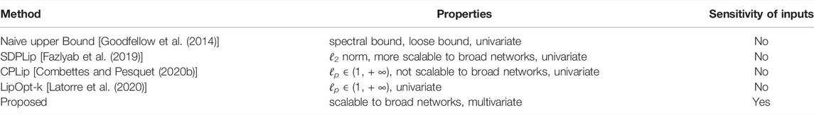
TABLE 1. Comparison of state-of-the-art Lipschitz estimation approaches vs the proposed one.

3 Weighted Lipschitz Constants for Sensitivity Analysis

To extend the theoretical results presented above on the evaluation of neural network stability through their Lipschitz regularity, we present in this section a new approach based on a suitable weighting operation performed in the computation of Lipschitz constants. This enables a multivariate sensitivity analysis of the neural network stability for individual inputs or groups of inputs. We will start by motivating this weighting from a statistical standpoint. Then we will define it in a more precise manner, before discussing its resulting mathematical properties.

3.1 Statistical Motivations

For tractability, assume that the perturbation at the network input is a realization of a zero-mean Gaussian distributed random vector $\mathsf{z}$ with N₀ × N₀ covariance matrix Σ ≻ 0. Then, its density upper level sets are defined as

$C_{\eta }=\left\{z\in {\mathbb{R}}^{N_0}\mid z^{\top }{\Sigma }^{-1}z\le \eta \right\},(38)$

for every $\left.\eta \in \right]0,+\infty \left[\right.$. The set C_η defines an ellipsoid where the probability density takes its highest values. More precisely, the probability for $\mathsf{z}$ to belong to this set is independent of Σ (Supplementary Appendix S1) and is equal to.

$\mathsf{P}\left(\mathsf{z}\in C_{\eta }\right)=\frac{\gamma \left(N_0/2,\eta /2\right)}{\mathrm{\Gamma }\left(N_0/2\right)},(39)$

where Γ is the gamma function and γ the lower (unnormalized) incomplete gamma function.

On the other hand, let us assume that the maximum standard deviation σ_max of the components of $\mathsf{z}$ (i.e., square root of the maximum diagonal element of matrix Σ) is small enough. If we suppose that the network T is differentiable in the neighborhood of a given input $x\in {\mathbb{R}}^{N_0}$, as the input perturbation is small enough, we can approximate the network output by the following expansion:

$T\left(x+z\right)\simeq T\left(x\right)+T^{\prime }\left(x\right)z.(40)$

Let us focus our attention on perturbations in C_η. By doing so, we impose some norm-bounded condition, which may appear more realistic for adversarial perturbations. Then, we will be interested in calculating

${\sup }_{z\in C_{\eta }}\Vert T\left(x+z\right)-T\left(x\right)\Vert \simeq {\sup }_{z\in C_{\eta }}\Vert T^{\prime }\left(x\right)z\Vert .(41)$

By making the variable change $z^{\prime }=z/\sqrt{\eta }$ and using Eq. 38,

$\begin{array}{ll}\hfill {\sup }_{z\in C_{\eta }}\Vert T\left(x+z\right)-T\left(x\right)\Vert & \simeq \sqrt{\eta }{\sup }_{z^{\prime }\in C_1}\Vert T^{\prime }\left(x\right)z^{\prime }\Vert \hfill \\ \hfill & =\sqrt{\eta }{\sup }_{\begin{array}{c}z\in {\mathbb{R}}^{N_0}\\ z^{\prime }\ne 0\end{array}}\frac{\Vert T^{\prime }\left(x\right)z^{\prime }\Vert }{\Vert z^{\prime }{\Vert }_{{\Sigma }^{-1}}}\hfill \\ \hfill & =\sqrt{\eta }{\sigma }_{\text{max}}{\sup }_{\begin{array}{c}{z}^{\prime }\in {\mathbb{R}}^{N_0}\\ z^{\prime }\ne 0\end{array}}\frac{\Vert T^{\prime }\left(x\right)z^{\prime }\Vert }{\Vert z^{\prime }{\Vert }_{{\mathrm{\Omega }}^{-1}}},\hfill \end{array}(42)$

where $\mathrm{\Omega }=\Sigma /{\sigma }_{\text{max}}^2$ and $\Vert \cdot {\Vert }_{{\mathrm{\Omega }}^{-1}}=\sqrt{{(\cdot )}^{\top }{\mathrm{\Omega }}^{-1}(\cdot )}$. This suggests that, in this context, the suitable subordinate matrix norm for computing the Lipschitz constant in Eq. 3 is obtained by weighting the Euclidean norm in the input space with Ω⁻¹. We can also deduce from Eq. 42, by setting z^″ = Ω^−1/2z′, that

$\begin{array}{ll}\hfill {\sup }_{z\in C_{\eta }}\Vert T\left(x+z\right)-T\left(x\right)\Vert & \simeq \sqrt{\eta }{\sigma }_{\text{max}}{\sup }_{\begin{array}{c}{z}^{″}\in {\mathbb{R}}^{N_0}\\ z^{″}\ne 0\end{array}}\frac{\Vert T^{\prime }\left(x\right){\mathrm{\Omega }}^{1/2}{z}^{″}\Vert }{\Vert z^{″}\Vert }\hfill \\ \hfill & =\sqrt{\eta }\Vert T^{\prime }\left(x\right){\Sigma }^{1/2}{\Vert }_{\text{S}}.\hfill \end{array}(43)$

On the other hand, based on the first-order approximation in Eq. 40, T(x + z) is approximately Gaussian with mean T(x) and covariance matrix T′(x)ΣT′(x)^⊤. As $\Vert T^{\prime }(x)\Sigma T^{\prime }{(x)}^{\top }{\Vert }_{\text{S}}=\Vert T^{\prime }(x){\Sigma }^{1/2}{\Vert }_{\text{S}}^2$, we see that another insightful interpretation of Eq. 43 is that, up to the scaling factor $\sqrt{\eta }$, it approximately delivers the square root of the spectral norm of the covariance matrix of the output perturbations.

3.2 New Definition of a Weighted Lipschitz constant

Based on the previous motivations, we propose to employ a weighted norm to define a Lipschitz constant of the network as follows:

Definition 1. Let Ω be an N0 × N0 symmetric positive definite real-valued matrix. We say that ${\theta}_{m}^{\upOmega}$ is an Ω-weighted norm Lipschitz constant of T as described in Figure 1 if

$\left(\forall \left(x,z\right)\in {\left({\mathbb{R}}^{N_0}\right)}^2\right)\Vert T\left(x+z\right)-T\left(z\right)\Vert \le {\theta }_m^{\mathrm{\Omega }}\Vert z{\Vert }_{{\mathrm{\Omega }}^{-1}}.(44)$

The above definition can be extended to non Euclidean norms by making use of exponents (p, q) ∈ (1,+∞)² and by replacing inequality Eq. 44 with

$\left(\forall \left(x,z\right)\in {\left({\mathbb{R}}^{N_0}\right)}^2\right)\Vert T\left(x+z\right)-T\left(z\right){\Vert }_q\le {\theta }_m^{\mathrm{\Omega }}\Vert {\mathrm{\Omega }}^{-1/2}z{\Vert }_p.(45)$

By changes of variable, this inequality can also be rewritten as.

$\left(\forall \left(x^{\prime },z^{\prime }\right)\in {\left({\mathbb{R}}^{N_0}\right)}^2\right)\Vert T\left({\mathrm{\Omega }}^{1/2}\left(x^{\prime }+z^{\prime }\right)\right)-T\left({\mathrm{\Omega }}^{1/2}{z}^{\prime }\right){\Vert }_q\le {\theta }_m^{\mathrm{\Omega }}\Vert z^{\prime }{\Vert }_p.(46)$

Therefore, we see that calculating ${\theta }_m^{\mathrm{\Omega }}$ is equivalent to derive a Lipschitz constant of the network T where an additional first linear layer Ω^1/2 has been added. Throughout the rest of this section, it will be assumed that, for every i ∈ (1, … , m−1) the activation operator R_i is separable and α_i-averaged. It then follows from Eq. 20 that an Ω-weighted norm Lipschitz constant of T is

${\vartheta }_m^{\mathrm{\Omega }}={\sup }_{\begin{array}{c}{\mathrm{\Lambda }}_1\in {\mathcal{D}}_{N_1}\left(\left\{2{\alpha }_1-\mathrm{1,1}\right\}\right),\\ ⋮,\\ {\mathrm{\Lambda }}_{m-1}\in {\mathcal{D}}_{N_{m-1}}\left(\left\{2{\alpha }_{m-1}-\mathrm{1,1}\right\}\right)\end{array}}\Vert W_m{\mathrm{\Lambda }}_{m-1}\dots ,{\mathrm{\Lambda }}_1{W}_1{\mathrm{\Omega }}^{1/2}{\Vert }_{p,q}.(47)$

Although all our derivations were based on the fact that Ω is positive definite, from the latter expression we see that, by continuous extension, ${\vartheta }_m^{\mathrm{\Omega }}$ can be defined when Ω is a singular matrix.

FIGURE 1

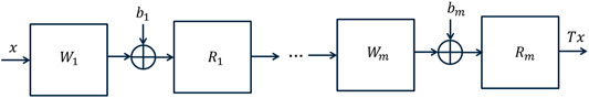
FIGURE 1. m-layered feedforward neural network architecture. For the ith-layer, W_i is the linear weight operator, b_i the bias vector, and R_i the activation operator.

3.3 Sensitivity with Respect to a Group of Inputs

In this section, we will be interested in a specific family of weighted norms associated with the set of matrices

$\left\{{\mathrm{\Omega }}_{ϵ,\mathbb{K}}\mid \varnothing \ne \mathbb{K}\subset \left\{1,\dots ,N_0\right\},\left.\left.ϵ\in \right]\mathrm{0,1}\right]\right\},$

defined, for every nonempty subset $\mathbb{K}$ of (1, … , N₀) and for every $\left.ϵ\in \right]\left.\mathrm{0,1}\right]$, as

${\mathrm{\Omega }}_{ϵ,\mathbb{K}}=\mathrm{Diag}\left({\sigma }_{ϵ,\mathbb{K},1}^2,\dots ,{\sigma }_{ϵ,\mathbb{K},N_0}^2\right),(48)$

where

$\left(\forall \ell \in \left\{1,\dots ,N_0\right\}\right){\sigma }_{ϵ,\mathbb{K},\ell }=\left\{\begin{array}{cc}1\hfill & \text{if}\ell \in \mathbb{K}\hfill \\ ϵ\hfill & \text{otherwise.}\hfill \end{array}\right.(49)$

If we come back to the statistical interpretation in Section 3.1, ${\mathrm{\Omega }}_{ϵ,\mathbb{K}}$ is then (up to a positive scale factor) the covariance matrix of a Gaussian random vector $\mathsf{z}$ with independent components⁴. The components with indices in $\mathbb{K}$ have a given variance ${\sigma }_{\text{max}}^2$ while the others have variance ${ϵ}^2{\sigma }_{\text{max}}^2$. Such a matrix thus provides a natural way of putting emphasis on the group of inputs with indices in $\mathbb{K}$. Thus, variables ${\vartheta }_m^{{\mathrm{\Omega }}_{ϵ,\mathbb{K}}}$ will be termed partial Lipschitz constants in the following.

The next proposition lists the main properties related to the use of such weighted norms for calculating Lipschitz constants. The proofs of these results are given in Supplementary Appendix S2.

Proposition 1. Let (p, q) ∈ (1,+∞)². For every nonempty subset $\mathbb{K}$ of (1, … , N₀) and for every $\left.ϵ\in \right]\left.\mathrm{0,1}\right]$, let ${\mathrm{\Omega }}_{ϵ,\mathbb{K}}$ be defined as above and let ${\vartheta }_m^{{\mathrm{\Omega }}_{ϵ,\mathbb{K}}}$ be defined by (47). Let ${\mathbb{K}}_0$ and ${\mathbb{K}}_1$ be nonempty subsets of (1, … , N₀). Then the following hold:

1) As ϵ → 0, ${\vartheta }_m^{{\mathrm{\Omega }}_{ϵ,{\mathbb{K}}_0}}$ converges to the Lipschitz constant of a network where all the inputs with indices out of ${\mathbb{K}}_0$ are kept constant.

2) ${\vartheta }_m^{{\mathrm{\Omega }}_{1,{\mathbb{K}}_0}}$ is equal to the global Lipschitz constant ϑ_m defined by Eq. 20.

3) Let $(ϵ,{ϵ}^{\prime })\left.\in \right]{\left.\mathrm{0,1}\right]}^2$. If ${\mathrm{\Omega }}_{ϵ,{\mathbb{K}}_0}⪯{\mathrm{\Omega }}_{{ϵ}^{\prime },{\mathbb{K}}_1}$, then ${\vartheta }_m^{{\mathrm{\Omega }}_{ϵ,{\mathbb{K}}_0}}\le {\vartheta }_m^{{\mathrm{\Omega }}_{{ϵ}^{\prime },{\mathbb{K}}_1}}$.

4) Function ${\vartheta }_m^{{\mathrm{\Omega }}_{\cdot ,{\mathbb{K}}_0}}\left.:\right]\left.\mathrm{0,1}\right]\to \left[0,+\infty \right.\left[:ϵ\mapsto {\vartheta }_m^{{\mathrm{\Omega }}_{ϵ,{\mathbb{K}}_0}}\right.$ is monotonically increasing.

5) Let $ϵ\left.\in \right]\left.\mathrm{0,1}\right]$. If ${\mathbb{K}}_0\subset {\mathbb{K}}_1$, then ${\vartheta }_m^{{\mathrm{\Omega }}_{ϵ,{\mathbb{K}}_0}}\le {\vartheta }_m^{{\mathrm{\Omega }}_{ϵ,{\mathbb{K}}_1}}$.

6) Let $\left.ϵ\in \right]\left.\mathrm{0,1}\right]$, let $K\in \mathbb{N}\backslash \{0\}$, and let

${\omega }_{K,ϵ}=\left(\genfrac{}{}{0.0pt}{}{N_0-1}{K-1}\right)\left(1+\left(\frac{N_0}{K}-1\right)ϵ\right).(50)$

We have

${\max }_{\begin{array}{c}\mathbb{K}\subset \left\{1,\dots ,N_0\right\}\\ card\mathbb{K}=K\end{array}}{\vartheta }_m^{{\mathrm{\Omega }}_{ϵ,\mathbb{K}}}\le {\vartheta }_m\le \frac{1}{{\omega }_{K,ϵ}}\sum _{\begin{array}{c}\mathbb{K}\subset \left\{1,\dots ,N_0\right\}\\ card\mathbb{K}=K\end{array}}{\vartheta }_m^{{\mathrm{\Omega }}_{ϵ,\mathbb{K}}}.(51)$

7) Let $\left.ϵ\in \right]\left.\mathrm{0,1}\right]$, let $\mathcal{P}$ be a partition of (1, … , N₀), and let.

${\omega }_{\mathcal{P},ϵ}=1+(card\mathcal{P}-1)ϵ.$

We have

${\max }_{\mathbb{K}\in \mathcal{P}}{\vartheta }_m^{{\mathrm{\Omega }}_{ϵ,\mathbb{K}}}\le {\vartheta }_m\le \frac{1}{{\omega }_{\mathcal{P},ϵ}}\sum _{\mathbb{K}\in \mathcal{P}}{\vartheta }_m^{{\mathrm{\Omega }}_{ϵ,\mathbb{K}}}.(52)$

8) Let ${\mathbb{K}}_2$ be such that ${\mathbb{K}}_1\cap {\mathbb{K}}_2\ne \varnothing$ and ${\mathbb{K}}_1\cup {\mathbb{K}}_2={\mathbb{K}}_0$. Let p∗ ∈ (1, + ∞) be such that 1/p + 1/p@ = 1 Then

${\vartheta }_m^{{\mathrm{\Omega }}_{ϵ,{\mathbb{K}}_0}}\le {\left({\left({\vartheta }_m^{{\mathrm{\Omega }}_{ϵ,{\mathbb{K}}_1}}\right)}^{p^{\ast }}+{\left({\vartheta }_m^{{\mathrm{\Omega }}_{ϵ,{\mathbb{K}}_2}}\right)}^{p^{\ast }}\right)}^{1/p^{\ast }}+o\left(ϵ\right).(53)$

Let us comment on these results. According to Property (i) in the limit case when ϵ → 0, only the inputs with indices in ${\mathbb{K}}_0$ are used in the computation of the associated Lipschitz constant. In turn, Property (ii) states that, when ϵ = 1, we recover the classical expression of a Lipschitz constant where the perturbations on all the inputs are taken into account. In addition, based on Property (iv), the evolution of ${\vartheta }_m^{{\mathrm{\Omega }}_{ϵ,{\mathbb{K}}_0}}$ when ϵ varies from 1 to 0 provides a way of assessing how the group of inputs indexed by ${\mathbb{K}}_0$ contributes to the overall Lipschitz behaviour of the network. Although one would expect that summing the Lipschitz constants obtained for each group of inputs would yield the global Lipschitz constant, Properties (vi) and (vii) show that this does not hold in general whatever the way the entries are split (possibly overlapping groups of given size K or disjoint groups of arbitrary size). Instead, after suitable normalization, such sums provide upper bounds on ϑ_m. Furthermore, it follows from (2), Eqs 51, 52 that the difference between these normalized sums and ϑ_m tends to vanish when ϵ increases.Note that, when looking at the sensitivity with respect to individual inputs, i.e., when the considered set of indices are singletons, both (6) (with K = 1) and (7) (with $\mathcal{P}=\{\{k\}\mid k\in \{1,\dots ,N_0\}\}$ lead to the same inequality

${\max }_{k\in \left\{1,\dots ,N_0\right\}}{\vartheta }_m^{{\mathrm{\Omega }}_{ϵ,\left\{k\right\}}}\le {\vartheta }_m\le \frac{1}{1+\left(N_0-1\right)ϵ}\sum _{k=1}^{N_0}{\vartheta }_m^{{\mathrm{\Omega }}_{ϵ,\left\{k\right\}}}.(54)$

4 Validation on Synthetic Data

4.1 Context

To highlight the need for advanced sensitivity analysis tools in the design of neural networks, we first study simple synthetic examples of polynomial systems for which we can calculate explicitly the partial Lipschitz constants. We generate input-output data for the defined systems, and train a fully connected model using a standard training, i.e., without any constraints. We compare this approach with a training subject to a spectral norm constraint on the layers.

Spectral Normalization: For safety critical tasks, Lipschitz constant and performance targets can be specified as engineering requirements, prior to network training. A Lipschitz target can be defined by a safety analysis of the acceptable perturbations for each output knowing the input range and it constitutes a current practice in many industries. Imposing this Lipschitz target can be done either by controlling the Lipschitz constant for each layer or for the whole network depending on the application at hand. Such a work for controlling the Lipschitz constant has been presented in (Serrurier et al., 2021) using Hinge regularization. In our experiments, we train networks while using a spectral normalization technique (Miyato et al., 2018) which has been proved to be effective in controlling Lipschitz properties in GANs. Given an m layer fully connected architecture and a Lipschitz target L, we can constrain the spectral norm of each layer to be less than $\sqrt[m]{L}$. According to Eq. 4, this ensures that the upper bound on the global Lipschitz constant is less than L.

For each training, we study the effect of input variables on the stability of the networks. As proposed in Section 3.3, for a given group of inputs with indices in $\mathbb{K}$, we will quantify the partial Lipschitz constant ${\vartheta }_m^{{\mathrm{\Omega }}_{ϵ,\mathbb{K}}}$. The obtained value of ${\vartheta }_m^{{\mathrm{\Omega }}_{ϵ,\mathbb{K}}}$ allows us to evaluate how the corresponding group of variables may potentially affect the stability of the network. For simplicity, in this section, we will focus on the limit case when ϵ = 0 (see the last remark in Section 3.2).

Partial Lipschitz constant values ${\vartheta }_m^{{\mathrm{\Omega }}_{0,\mathbb{K}}}$, for all possible choices for $\mathbb{K}$, are computed using the numerical method described in Section 2.2 and compared with the theoretical values derived in the following subsection. More details on the models are also provided in these sections.

4.2 Polynomial Systems

We consider regression problems where the data is synthesized by a second-order multivariate polynomial. The system to be modelled is thus described by the following function:

$\left(\forall \left({\xi }_1,\dots ,{\xi }_{N_0}\right)\in {\mathbb{R}}^{N_0}\right)f\left({\xi }_1,\dots ,{\xi }_{N_0}\right)=\sum _{k=1}^{N_0}{a}_k{\xi }_k+\sum _{k=1}^{N_0}\sum _{l=1}^{N_0}{b}_{k,l}{\xi }_k{\xi }_l,(55)$

where ${(a_k)}_{k\in N_0}$ and ${(b_{k,l})}_{1\le k,l\le N_0}$ are the real-valued polynomial coefficients. Note that, such a polynomial system is generally not Lipschitz-continuous. The Lipschitz-continuity property only holds on every compact set. Subsequently, we will thus study this system on the hypercube ${[-M,M]}^{N_0}$ with M > 0.

The explicit values of the partial Lipschitz constant on this domain can be derived as follows. We first calculate the gradient of f

$\nabla f\left({\xi }_1,\dots ,{\xi }_{N_0}\right)={\left({\partial }_{k}f\left({\xi }_1,\dots ,{\xi }_{N_0}\right)\right)}_{1\le k\le N_0},(56)$

where, for every k ∈ (1, … , N₀), ∂_kf denotes the partial derivative w.r.t. the k-th variable given by

${\partial }_{k}f\left({\xi }_1,\dots ,{\xi }_{N_0}\right)=a_k+\sum _{l=1}^{N_0}\left(b_{k,l}+b_{l,k}\right){\xi }_l.(57)$

For every $\mathbb{K}\subset \{1,\dots ,N_0\}$, the partial Lipschitz constant ${\mathring{\vartheta }}^{{\mathrm{\Omega }}_{0,\mathbb{K}}}$ of the polynomial system (restricted to ${[-M,M]}^{N_0}$) w.r.t. the group of variables with indices in $\mathbb{K}$ is then equal to.

${\mathring{\vartheta }}^{{\mathrm{\Omega }}_{0,\mathbb{K}}}={\sup }_{\left({\xi }_1,\dots ,{\xi }_{N_0}\right)\in {\left[-M,M\right]}^{N_0}}\sqrt{{\lambda }_{{\mathrm{\Omega }}_{0,\mathbb{K}}}\left({\xi }_1,\dots ,{\xi }_{N_0}\right)},(58)$

where, for every diagonal matrix $\mathrm{\Lambda }=\mathrm{Diag}({\epsilon }_1^2,\dots ,{\epsilon }_{N_0}^2)$ with $({\epsilon }_1,\dots ,{\epsilon }_{N_0})\in \left[0,+\infty \right.{\left[\right.}^{N_0}$,

$\begin{array}{ll}\hfill {\lambda }_{\mathrm{\Lambda }}\left({\xi }_1,\dots ,{\xi }_{N_0}\right)& =\Vert {\left(\nabla f\left({\xi }_1,\dots ,{\xi }_{N_0}\right)\right)}^{\top }{\mathrm{\Lambda }}^{1/2}{\Vert }^2\hfill \\ \hfill & =\sum _{k=1}^{N_0}{\epsilon }_k{\left({\partial }_{k}f\left({\xi }_1,\dots ,{\xi }_{N_0}\right)\right)}^2.\hfill \end{array}(59)$

Since the partial derivatives in Eq. 57 are affine functions of the variables $({\xi }_1,\dots ,{\xi }_{N_0})$, λ_Λ is a convex function. We deduce that the supremum in Eq. 58 is attained when ${\xi }_1=\pm M,\dots ,{\xi }_{N_0}=\pm M$, so that ${\mathring{\vartheta }}^{{\mathrm{\Omega }}_{0,\mathbb{K}}}$ can be computed by looking for the maximum of a finite number of values.

4.3 Numerical Results

In our numerical experiments, we consider a toy example corresponding to N₀ = 3 and

$\left(\forall \left({\xi }_1,{\xi }_2,{\xi }_3\right)\in {\mathbb{R}}^3\right)f\left({\xi }_1,{\xi }_2,{\xi }_3\right)={\xi }_1+100{\xi }_3-{\xi }_2^2+\gamma {\xi }_1{\xi }_3,(60)$

where $\gamma \in \left[0,+\infty \right.\left[\right.$. We deduce from Eq. 59 that

${\lambda }_{\mathrm{\Lambda }}\left({\xi }_1,{\xi }_2,{\xi }_3\right)={\epsilon }_1{\left(1+\gamma {\xi }_3\right)}^2+4{\epsilon }_2{\xi }_2^2+{\epsilon }_3{\left(100+\gamma {\xi }_1\right)}^2(61)$

and, consequently,

${\sup }_{\left({\xi }_1,{\xi }_2,{\xi }_3\right)\in {\left[-M,M\right]}^3}{\lambda }_{\mathrm{\Lambda }}\left({\xi }_1,{\xi }_2,{\xi }_3\right)={\epsilon }_1{\left(1+\gamma M\right)}^2+4{\epsilon }_2{M}^2+{\epsilon }_3{\left(100+\gamma M\right)}^2.(62)$

By looking at the seven possible binary values of (ɛ₁, ɛ₂, ɛ₃) ≠ (0, 0, 0), we thus calculate the Lipschitz constant of f with respect to each group of inputs. For example,

• if ɛ₁ = 1, ɛ = 0, ɛ₃ = 0, we calculate ${\mathring{\vartheta }}^{{\mathrm{\Omega }}_{0,\mathbb{K}}}$ with $\mathbb{K}=\{1\}$, i.e., evaluate the sensitivity w.r.t. the first variable

• if ɛ₁ = ɛ₂ = 1, ɛ₃ = 0, we calculate ${\mathring{\vartheta }}^{{\mathrm{\Omega }}_{0,\mathbb{K}}}$ with $\mathbb{K}=\{\mathrm{1,2}\}$, i.e., evaluate the joint sensitivity w.r.t. the first and second variables;

• if ɛ₁ = ɛ₂ = ɛ₃ = 1, we calculate ${\mathring{\vartheta }}^{{\mathrm{\Omega }}_{0,\mathbb{K}}}$ with $\mathbb{K}=\{\mathrm{1,2,3}\}$, i.e., evaluate the sensitivity w.r.t. all the variables (global Lipschitz constant).

These Lipschitz constants allow us to evaluate the intrinsic dynamics of the system, that is how it responds when its inputs vary.

Our interest will be now to evaluate how this dynamics is modified when the system is modelled by a neural network. To do so, three systems are studied by choosing γ ∈ (0, 1/10, 1) and M = 50. We generate 5,000 data samples from each system, the input values being drawn independently from a random uniform distribution. While training the neural networks, the dataset is divided with a ratio of 4:1 into training and testing samples. The input is normalized using its mean and standard deviation, while the output is max-normalized. We build neural networks for approximating the systems using two hidden layers (m = 3) with a number of hidden neurons equal to 30 in each layer and ReLU activation functions. The training loss is the mean square error.

For different values of γ, we report the values of the partial Lipschitz constants in Tables 2, 3, 4. The variable ${\theta }_{\mathbb{K}}$ corresponds to ${\mathring{\vartheta }}^{{\mathrm{\Omega }}_{0,\mathbb{K}}}$ for the analytical value we derived from previous formulas, whereas it corresponds to the Lipschitz constant ${\vartheta }_3^{{\mathrm{\Omega }}_{0,\mathbb{K}}}$, when computed for the neural network trained either in a standard manner or with a spectral normalization constraint. The value of L used in the spectral normalization was adjusted to obtain a similar global Lipschitz constant to the polynomial system. In the caption, we also indicate the accuracy in terms of normalized mean square error (NMSE) and normalized mean absolute error (NMAE). These values are slightly higher for constrained training, but remain quite small.

TABLE 2

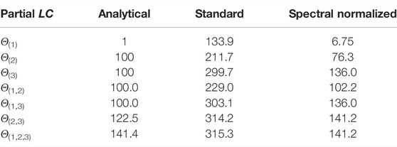
TABLE 2. Comparison of Lipschitz constant values when γ = 0. Test performance for standard training: NMSE = 0.007, NMAE = 0.005, for spectral normalization: NMSE = 0.011, NMAE = 0.009.

TABLE 3

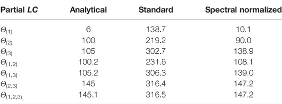
TABLE 3. Comparison of Lipschitz constant values when γ = 1/10. Test performance for standard training: NMSE = 0.006, NMAE = 0.005, for spectral normalization: NMSE = 0.009, NMAE = 0.007.

TABLE 4

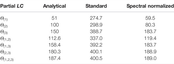
TABLE 4. Comparison of Lipschitz constant values when γ = 1. Test performance for standard training: NMSE = 0.006, MAE = 0.005, for spectral normalization: NMSE = 0.014, NMAE = 0.009.

Comments on the results:

• In general, ξ₃ impacts the output of this system the most, and (ξ₂, ξ₃) mainly account for the global dynamics of the system.

• With standard training, we see that there exists a significant increase of the sensitivity with respect to the input variations, so making the neural network vulnerable to adversarial perturbations.

• By using spectral normalization, it is possible to constrain the global Lipschitz constant of the system to be close to the analytical global value while keeping a good accuracy. One may however notice an increase of the sensitivity to ξ₁ and ξ₃, and a decrease of the sensitivity to ξ₂ with respect to the original system.

• For all the three models, the values obtained with neural networks follow the same trend, for different groups of inputs, as those observed with the analytical values.

• Although the Lipschitz constant of the neural networks is computed on the whole space and the one of the system on (−50,50)³, our Lipschitz estimates appear to be consistent without resorting to a local analysis.

These observations emphasize the importance of controlling the Lipschitz constant of neural network models through specific training strategies. In addition, we see that evaluating the Lipschitz constant with respect to groups of inputs allow us to have a better understanding of the behaviour of the models.

In this section, we have discussed the proposed method for synthetic datasets. In the next section, the sensitivity analysis will be made on widely used open source datasets and an industrial dataset.

5 Application on Different Use Cases

5.1 Datasets and Network Description

We study four regression problems involving tabular datasets to showcase our proposed multivariate analysis of the stability of neural networks. Tabular data take advantage of heterogeneous sources of information coming from different sensors or data collection processes. We apply our methods on widely used tabular datasets: 1) Combined Cycle Power Plant dataset ⁵ which has 4 attributes with 9,568 instances; 2) Auto MPG dataset ⁶ consists of 398 instances with 7 attributes; 3) Boston Housing dataset ⁷ consists of 506 instances with 13 attributes. For Combined Power Plant and Auto MPG datasets, we solve a regression problem with a single output, whereas for Boston Housing dataset we consider a two-output regression problem with “price” and “ptratio” as the output variables. The attributes in the dataset are a combination of continuous and categorical. The datasets are divided with a ratio of 4:1 between training and test data.

Thales Air Mobility industrial application represents the prediction of the Estimated Time En-route (ETE), meaning the time spent by an aircraft between the take-off and landing, considering a number of variables as described in Table 5. The application is important in air traffic flow management, which is an activity area where safety is critical. The purpose of the proposed sensitivity analysis is thus to help engineers in building safe by design models complying with given safety stability targets. The dataset consists of 2,219,097 training, 739,639 validation, and 739,891 test samples.

TABLE 5

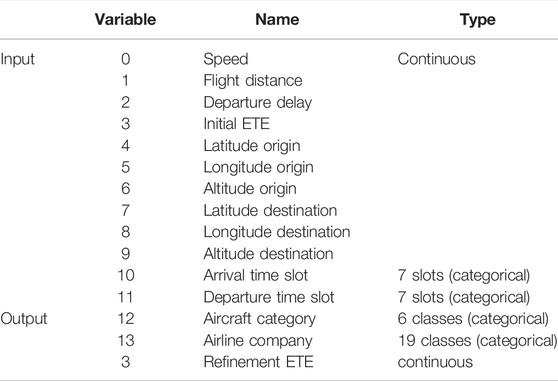
TABLE 5. Input and output variables description for the Thales Air Mobility industrial application dataset.

For all the models, we build fully connected networks with ReLU⁸ activation function on all the hidden layers, except the last one. The models are trained on Keras with Tensorflow backend. The initializers are set to Glorot uniform. The network architecture of the different models, number of layers, and neurons are tabulated in Table 6. Combined Cycle Power Plant dataset with (10, 6) network architecture is trained with two hidden layers having 10 and 6 hidden neurons, respectively. For Thales Air Mobility industrial application [10 × (30)] implies that the neural network has 10 hidden layers with 30 neurons each.

TABLE 6

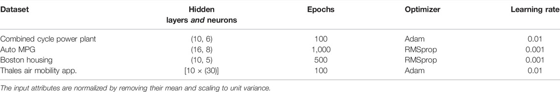
TABLE 6. Network Architecture and training setup for different datasets.

5.2 Sensitivity Analysis with Respect to Each Input

In this section we study the effect of input variables on the stability of the networks. More specifically, we study the effect of input variations on the stability of the networks by quantifying ${\vartheta }_m^{{\mathrm{\Omega }}_{ϵ,\mathbb{K}}}$ with $\left.ϵ\in \right]\left.\mathrm{0,1}\right]$, for various choices of $\mathbb{K}$, instead of a global Lipschitz constant accounting for the influence of the whole set of inputs. The obtained value of ${\vartheta }_m^{{\mathrm{\Omega }}_{ϵ,\mathbb{K}}}$ allows us to evaluate how the corresponding group of variables may potentially affect the stability of the network. By performing this analysis for several choices of $\mathbb{K}$, we thus generate a multivariate analysis of the Lipschitz regularity of the network.

As shown by Proposition 1, varying the ϵ parameter is also insightful since it allows us to measure how the network behaves when input perturbations are gradually more concentrated on a given subset of inputs.

Although our approach can be applied to groups of inputs, for simplicity in this section, we will focus on the case when the sets $\mathbb{K}$ reduce to singletons. In this context, we propose a new representation for displaying the results of the Lipschitz analysis of a neural network. More precisely, we plot the values of ${({\vartheta }_m^{{\mathrm{\Omega }}_{ϵ,\{k\}}})}_{1\le k\le N_0}$ on a star or radar chart where each branch of the star corresponds to the index k of an input. For each value of ϵ, a new plot is obtained which is displayed in a specific color. Note that, according to Proposition 3(iv), the plots generated for different ϵ values cannot cross. When ϵ = 1, we obtain an “isotropic” representation whose “radius” corresponds to the global Lipschitz constant ϑ_m of the network. This representation is called a Lipschitz star. All the results of our analysis will be displayed with this representation.

For each dataset, we first perform a standard training when designing the network. To facilitate comparisons, the Lipschitz star of the network trained in such standard manner is presented as the first subplot of all the figures in the paper. Next, we show the variation in terms of input sensitivity, when 1) a Lipschitz target is imposed, and 2) when an adversarial training of the networks is performed. The network architecture remains unchanged, for all our experiments and each dataset, as indicated in Section 5.1. All the Lipschitz constants for each value of ϵ are calculated using LipSDP-Neuron (Fazlyab et al., 2019). Since an increased stability may come at the price of a loss of accuracy (Tsipras et al., 2018a), we also report the performance of the networks on test datasets in terms of MAE (Mean Absolute Error) for each of the Lipschitz star plot.

5.3 Effect of Training With Specified Lipschitz Target

Spectral norm constrained training is performed as explained in Section 4.1. The results are shown for our three datasets in Figures 2–5. On these plots, we can observe a shrinkage of the Lipschitz stars following the reduction of the target Lipschitz value. Interestingly, improving stability does not affect significantly the performance of the networks. Let us comment on the last use case in light of the obtained results.

FIGURE 2

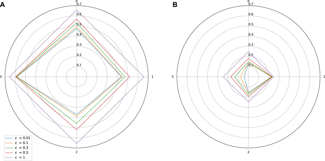
FIGURE 2. Sensitivity w.r.t. to each input on Combined Cycle Power Plant dataset. Influence of a spectral normalization constraint. (A) Standard training: Lipschitz constant = 0.66, MAE = 0.007, (B) With spectral normalization: Lipschitz constant = 0.25, MAE = 0.0066.

FIGURE 3

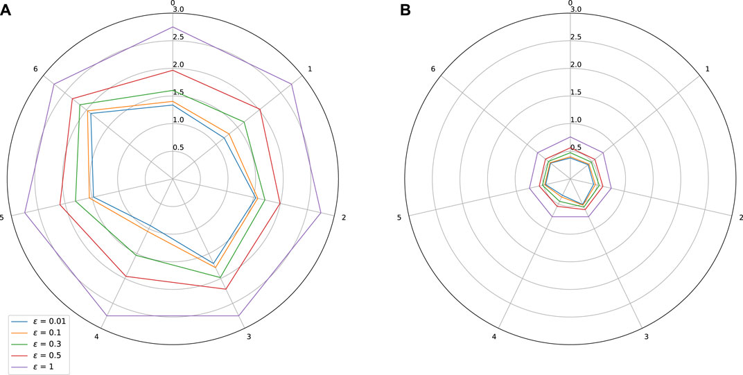
FIGURE 3. Sensitivity w.r.t. to each input on Auto MPG dataset. Influence of a spectral normalization constraint. (A) Standard training: Lipschitz constant = 2.75, MAE = 0.05, (B) With spectral normalization: Lipschitz constant = 0.76, MAE = 0.04.

FIGURE 4

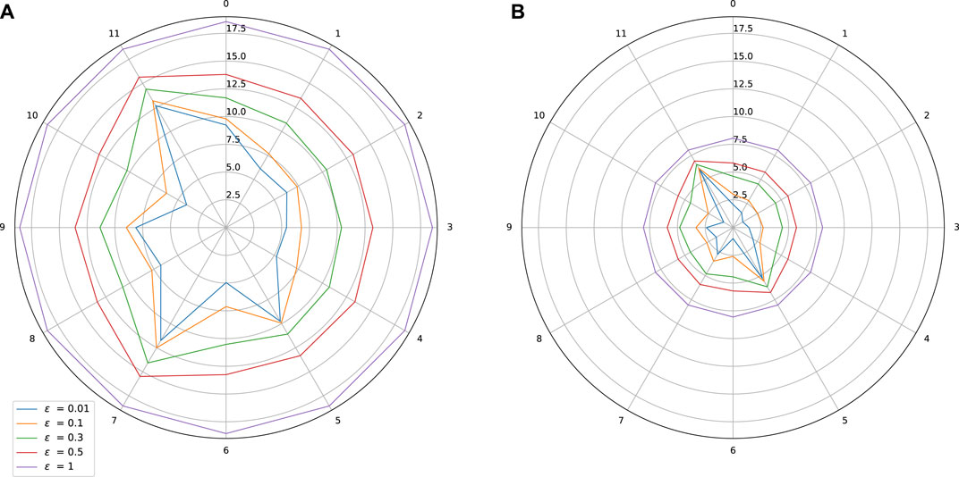
FIGURE 4. Sensitivity w.r.t. to each input on Boston Housing dataset. Influence of a spectral normalization constraint. (A) Standard training: Lipschitz constant = 18.56, MAE(y₁) = 2.45, MAE(y₂) = 1.41, (B) With spectral normalization: Lipschitz constant = 8.06, MAE(y₁) = 2.96, MAE(y₂) = 1.35.

FIGURE 5

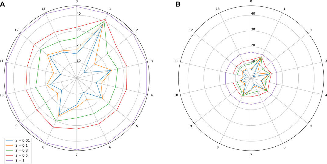
FIGURE 5. Sensitivity w.r.t. to each input on Thales Air Mobility industrial application. Influence of a spectral normalization constraint. (A) Standard training: Lipschitz constant = 45.46, MAE = 496.37 (s), (B) With spectral normalization constraint: Lipschitz constant = 16.62, MAE = 478.88 (s).

Comments on the Thales Air Mobility industrial application From the star plots, it is clear that the various variables have a quite different effect on the Lipschitz behavior of the network. This is an expected outcome since these variables carry a different amount of information captured by learning. From Figure 5 we observe that variables 1—Flight Distance and 3—Initial ETE play a prominent role, while variables 5—Longitude Origin, and 8—Longitude Destination are also sensitive. Some plausible explanations for these facts are mentioned below.

• Flight distance: The impact of a change of this input can be significant since because of air traffic management separation rules, the commercial aircrafts cannot freely increase their speed to minimize the impact of a longer flight distance.

• Initial ETE: Modifying this input is equivalent to changing the initial conditions, which will have a significant impact. It is possible, in the worst case scenario, to accumulate other perturbations coming from other coupled inputs and parameters (e.g., weather conditions) and this is probably the reason why the partial Lipschitz constant is very high, and close to the global Lipschitz constant.

• Longitude origin and destination parameters: These parameters are related to different continents and even countries of the origin and destination airports and probably with different qualities of air traffic equipment.

5.4 Effect of Adversarial Training

Generating adversarial attacks and performing adversarial training constitute popular methods in designing robust neural networks. However, these techniques have received less attention for regression tasks, since most of the works deal with classification tasks (Goodfellow et al., 2015; Kurakin et al., 2018; Eykholt et al., 2018). Also, most of the existing works in the deep learning literature are for standard signal/image processing problems, whereas there are only few works handling tabular data (Zhang et al., 2016; Ke et al., 2018). One noticeable exception is (Ballet et al., 2019) which investigates problems related to adversarial attacks for classification tasks involving tabular data. Since our applications are related to regression problems for which few existing works are directly applicable, we designed a specific adversarial training method. More specifically, for a given amplitude of the adversarial noise and for each sample in the training set, we generate the worst attack based on the spectral properties of the Jacobian of the network, computed by backpropagation at this point. At each epoch of the adversarial training procedure, we solve the underlying minmax problem (Tu et al., 2019). More details on the generation of adversarial attacks for regression attacks can be found in (Gupta et al., 2021).

The generated adversarial attacks from the trained model at the previous epoch are successively concatenated to the training set for the next training epoch, much like in standard adversarial training practices using FGSM (Goodfellow et al., 2015) and Deepfool (Moosavi-Dezfooli et al., 2016) attacks. While generating adversarial attacks on tabular data, some of the variables may be more susceptible to attacks than others. The authors of (Ballet et al., 2019) take care of this aspect by using a feature importance vector. They also only attack the continuous variables, disregarding categorical ones while generating attacks. For the Power plant and Boston Housing datasets, we attack all the four input variables, while on the MPG dataset, we attack only the continuous variables. For the industrial dataset, we generate attacks for the five most sensitive input variables. We also tried attacking all the variables of the dataset but this was not observed to be more efficient. The results in form of Lipschitz star are given in Figures 6–9.

FIGURE 6

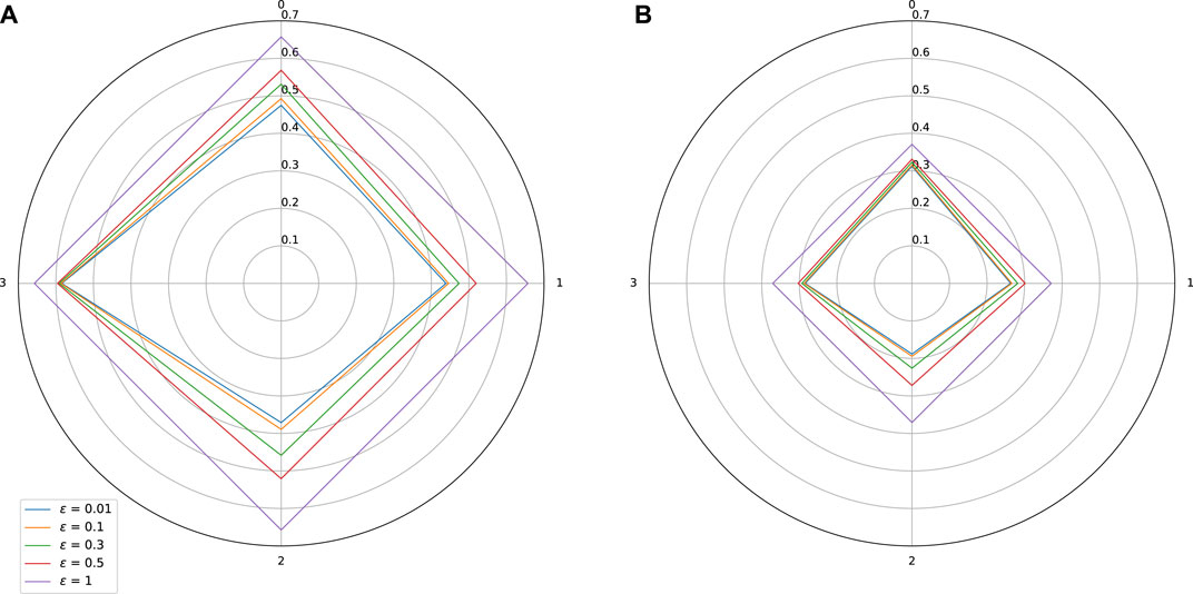
FIGURE 6. Sensitivity w.r.t. to each input on Combined Cycle Power Plant dataset. Effect of adversarial training. (A) Standard training: Lipschitz constant = 0.657, MAE = 0.007, (B) Adversarial training: Lipschitz constant = 0.37, MAE = 0.0068.

FIGURE 7

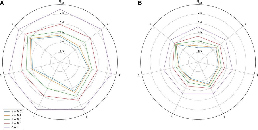
FIGURE 7. Sensitivity w.r.t. to each input on Auto MPG dataset. Effect of adversarial training. (A) Standard training: Lipschitz constant = 2.75, MAE = 0.05, (B) Adversarial training: Lipschitz constant = 1.84, MAE = 0.042.

FIGURE 8

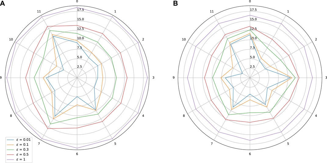
FIGURE 8. Sensitivity w.r.t. to each input on Boston Housing dataset. Effect of adversarial training. (A) Standard training: Lipschitz = 18.56, MAE(y₁) = 2.45, MAE(y₂) = 1.41, (B) Adversarial training: Lipschitz constant = 16.50, MAE(y₁) = 2.35 MAE(y₂) = 1.32.

FIGURE 9

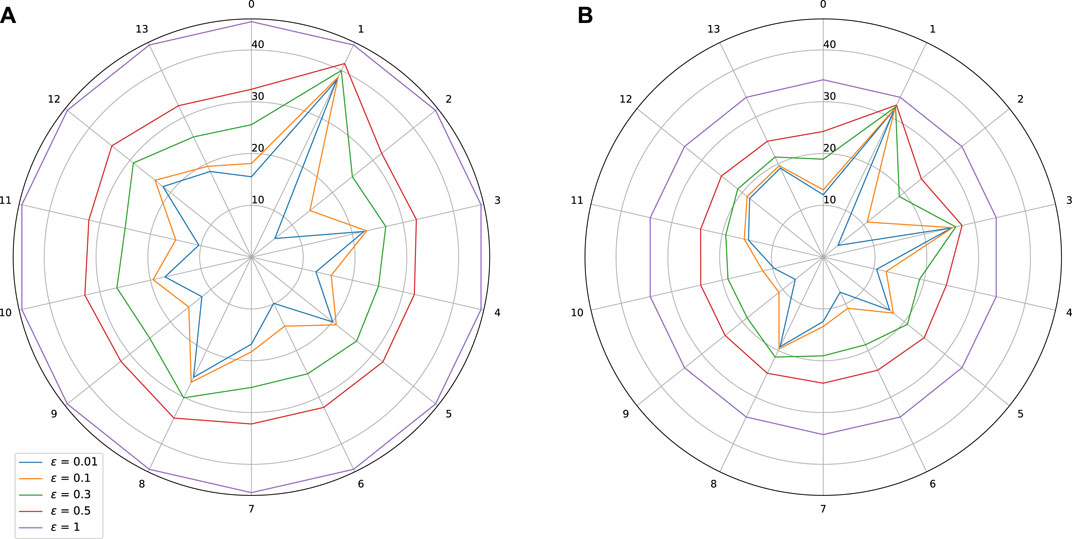
FIGURE 9. Sensitivity w.r.t. to each input on Thales Air Mobility industrial application. Effect of adversarial training. (A) Standard training: Lipschitz = 45.47, MAE = 496.37 (s), Adversarial training. (B) Lipschitz = 34.26, MAE = 494.7 (s).

As expected, adversarial training leads to a shrinkage of the star plots, which indicates a better control on the stability of the trained models, while also improving slightly the MAE. In the test we did, we observe however that our adversarial training procedure is globally less efficient than the spectral normalization technique.

5.5 Sensitivity w.r.t. Pair of Variables

We now consider the case when the set $\mathbb{K}$ contains pairs of elements. We first show the corresponding Partial Lipschitz constants using a Lipschitz star representation in Figure 10, for the different datasets we have discussed in the article. Vertices in the Lipschitz star represent the obtained Lipschitz constant value ${\vartheta }_m^{{\mathrm{\Omega }}_{ϵ,\mathbb{K}}}$ for all possible combinations of pair of variables with varying values of ϵ, i.e., it represents the sensitivity w.r.t. to that particular pair.

FIGURE 10

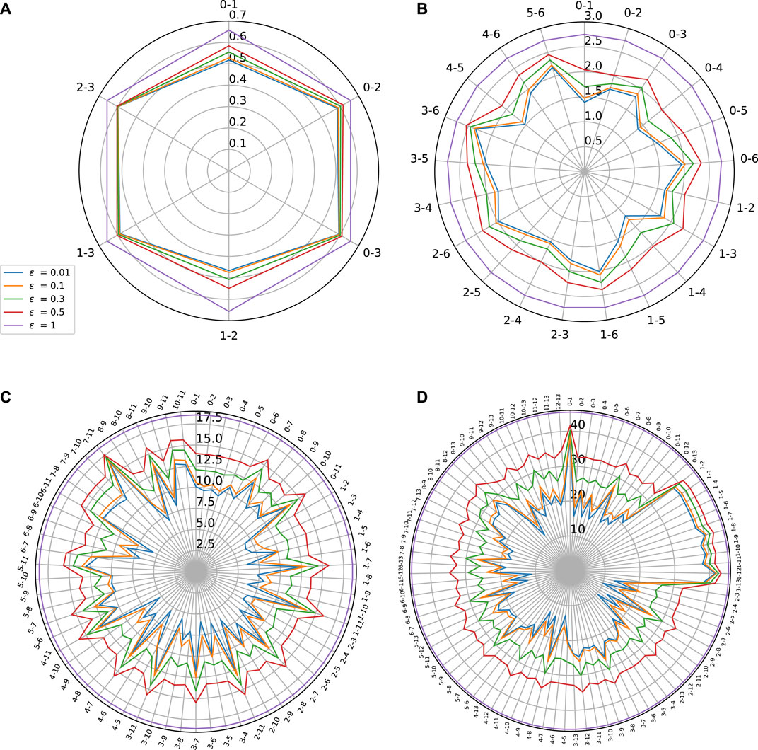
FIGURE 10. Sensitivity w.r.t to pair of variables on (A) Combined Power Plant dataset (B) Auto MPG Dataset (C) Boston Housing dataset and (D) Thales Air Mobility industrial application.

As shown by Figure 10, this Lipschitz star representation can be useful for displaying the influence of groups of variables instead of single ones. This may be of high interest when the number of inputs is large, especially if they can be grouped into variables belonging to a given class having a specific physical meaning (e.g., electrical variables versus mechanical ones). Such Lipschitz star representation might however not be very insightful for identifying the coupling that may exist between the variables within a given group. For example, it may happen that, considered together, two variables yield an increased sensitivity than the sensitivity of each of them individually. The reason why we need to find a better way for highlighting these coupling effects is related to Proposition 3(v) which states that, for every $\left.ϵ\in \right]\left.\mathrm{0,1}\right]$ and $(k,\ell )\in {\{1,\dots ,N_0\}}^2$,

$\max \left\{{\vartheta }_m^{{\mathrm{\Omega }}_{ϵ,\left\{k\right\}}},{\vartheta }_m^{{\mathrm{\Omega }}_{ϵ,\left\{\ell \right\}}}\right\}\le {\vartheta }_m^{{\mathrm{\Omega }}_{ϵ,\left\{k,\ell \right\}}}.(63)$

This property means that, when considering a pair of inputs, the one with the highest partial Lipschitz constant will “dominate” the other. To circumvent this difficulty and make our analysis more interpretable, we can think of normalizing the Lipschitz constant in a suitable manner. Such a strategy is a common practice in statistics when, for example, the covariance of a pair of variables is normalized by the product of their standard deviations to define their correlation factor. Once again, we can take advantage of the properties established in Proposition 3 to provide us a guideline to perform this normalization. In addition to Eq. 63, according to Property (viii),

$\begin{array}{ll}\hfill {\vartheta }_m^{{\mathrm{\Omega }}_{ϵ,\left\{k,\ell \right\}}}& \le {\left({\left({\vartheta }_m^{{\mathrm{\Omega }}_{ϵ,\left\{k\right\}}}\right)}^{p^{*}}+{\left({\vartheta }_m^{{\mathrm{\Omega }}_{ϵ,\left\{\ell \right\}}}\right)}^{p^{\ast }}\right)}^{1/p^{\ast }}+o\left(ϵ\right)\hfill \\ \hfill & \le 2^{1/p^{\ast }}\max \left\{{\vartheta }_m^{{\mathrm{\Omega }}_{ϵ,\left\{k\right\}}},{\vartheta }_m^{{\mathrm{\Omega }}_{ϵ,\left\{\ell \right\}}}\right\}+o\left(ϵ\right).\hfill \end{array}(64)$

The two previous inequalities suggest to normalize the Lipschitz constant for pairs of inputs by defining

${\tilde{\vartheta }}_m^{{\mathrm{\Omega }}_{ϵ,\left\{k,\ell \right\}}}=\frac{1}{2^{1/p^{\ast }}-1}\left(\frac{{\vartheta }_m^{{\mathrm{\Omega }}_{ϵ,\left\{k,\ell \right\}}}}{\max \left\{{\vartheta }_m^{{\mathrm{\Omega }}_{ϵ,\left\{k\right\}}},{\vartheta }_m^{{\mathrm{\Omega }}_{ϵ,\left\{\ell \right\}}}\right\}}-1\right).(65)$

Indeed, when ϵ is close to zero, Eqs 63–65 show that ${\tilde{\vartheta }}_m^{{\mathrm{\Omega }}_{ϵ,\{k,\ell \}}}\in [\mathrm{0,1}]$. Note that, for the diagonal terms, ${\tilde{\vartheta }}_m^{{\mathrm{\Omega }}_{ϵ,\{k,k\}}}=0$. The higher ${\tilde{\vartheta }}_m^{{\mathrm{\Omega }}_{ϵ,\{k,\ell \}}}$, the higher the gain in sensitivity due to the coupling between k and ℓ. The normalized values for the different datasets are reported in Table 7.

TABLE 7

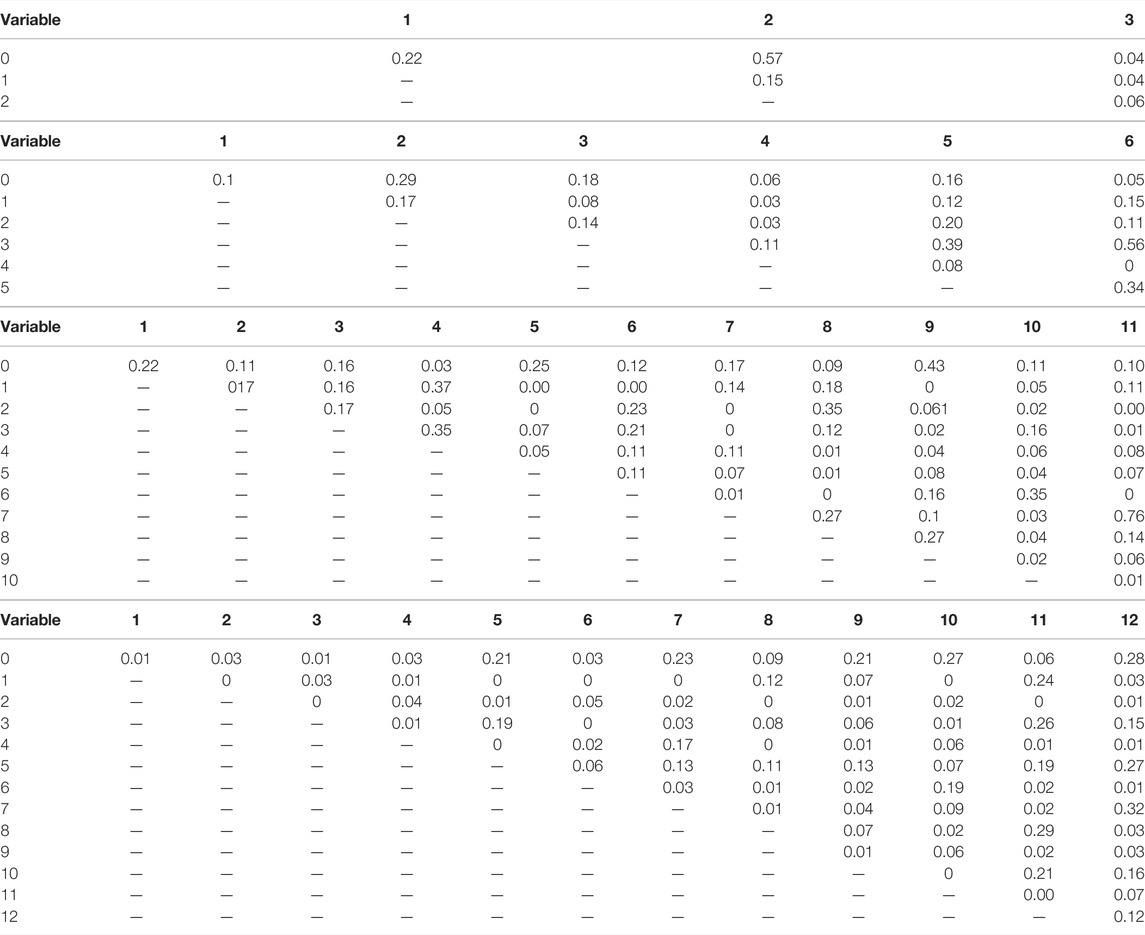
TABLE 7. Second order normalized coupling matrix with ϵ = 0.001 on (A) Combined Power Plant Dataset (B) Auto MPG Dataset (C) Boston Housing Dataset and (D) Thales Air Mobility industrial application.

5.6 Interpretation of the Results

We summarize some important observations/properties concerning the stability of the NNs which can be drawn from training on different datasets and leveraging the quantitative tools we have proposed in this article.

a) Combined Power Plant Dataset

• “3—Exhaust Vacuum” is the most sensitive variable out of the four variables.

• We observe for any variable coupled with “3” gives a higher partial Lipschitz constant.

• From Table 7A, we see that the effect is mostly caused by the sensitivity of “3” and there is no gain when coupled with other variables. Hence, “3” dominates the overall sensitivity of the NN.

• On the other hand, we observe that, “0” when coupled with “1” and “2” becomes more sensitive as evidenced by the gain in Table 7A.

b) Auto MPG Dataset

• Variable “6—Origin” and “3—Weight” are the most sensitive variables.

• The values of partial Lipschitz constant peak when the other variables are coupled with “3” or “6”.

• From Table 7B, we see that most of the values coupled with either “3” or “6” are close to zero, except when “3” and “6” are coupled together. Also, we see an exception when “5” is coupled with either “3” or “6”. This suggests that altogether “3”, “5”, and “6” have a higher impact on the stability of the network.

c) Boston Housing Dataset

• Variable “7—DIS” and “11—LSTAT” are the most sensitive variables.

• We observe a high partial Lipschitz constant when coupling any variables with “7” or “11”.

• From Table 7C, we see that all the values for both “7” and “11” coupled with other variables are close to zero, except when “7” and “11” are jointly considered. Hence, “7” and “11” dominate the sensitivity of the NN.

• We observe from the table of normalized values, that “2–9” have a higher impact on the sensitivity of the NN when coupled. Similar observation can be made for pairs “2–8”,“1–4”,“3–4”.

d) Thales Air Mobility industrial application

• Variable “1—Flight distance”,“3—Initial ETE”, and “8—Longitude Destination” are the most sensitive variables.

• We see peaks in the partial Lipschitz constant values when these highly sensitive variables are coupled with other variables.

• But when analyzing the normalized tables, it becomes clear that the gain is mostly due to these sensitive variables.

• We also observe from Table 7D, an increased sensitivity of “0” when coupled with other variables “5”, “7”, “10”, “11”, and “13”.

6 Conclusion

We have proposed a new multivariate analysis of the Lipschitz regularity of a neural network. Our approach, whose theoretical foundations are given in Section 3, allows the sensitivity with respect to any group of inputs to be highlighted. We have introduced a new “Lipschitz star” representation which is helpful to display how each input or group of inputs contributes to the global Lipschitz behaviour of a network. The use of these tools has been illustrated on four regression use cases involving tabular data. The improvements brought by two robust training methods (training subject to Lipschitz bounds and adversarial training) have been measured. More generally the proposed methodology is applicable to various machine learning tasks to build “safe-by-design” models where heterogeneous/multimodal/multi-omic data can be used.

Data Availability Statement

The industrial dataset presented in this article is not readily available because the dataset is internal to Thales. Further inquiries should be directed to kavya.gupta100@gmail.com. All other datasets are readily available from the following: https://archive.ics.uci.edu/ml/datasets/Combined+Cycle+Power+Plant; https://archive.ics.uci.edu/ml/datasets/auto+mpg; https://www.cs.toronto.edu/∼delve/data/boston/bostonDetail.html.

Author Contributions

KG—Doctoral student handling the processing of the datasets, coding of the tools proposed, optimization of the results and writing of the article. FK—Thales advisor of the doctoral student. Responsible for procuring industrial datasets and technical advises on the experimentation and better utilization of tools, editing of the article. BP-P—Thales advisor of the doctoral student. Responsible for procuring industrial datasets and technical advises on the experimentation.and better utilization of tools, editing of the article. J-CP—Academic advisor responsible mathematical proofs of the work presented in the article and writing of the article. FM—Academic advisor responsible for editing the article.

Funding

Doctoral thesis of KG is funded by l’Association Nationale de la Recherche et de la Technologie (ANRT) and Thales LAS France under CIFRE convention. Part of this work was supported by the ANR Research and Teaching Chair in Artificial Intelligence, BRIDGEABLE.

Conflict of Interest

KG, FK and BP-P were employed by the company Thales LAS France.

The remaining authors declare that the research was conducted in the absence of any commercial or financial relationships that could be construed as a potential conflict of interest.

Publisher’s Note

All claims expressed in this article are solely those of the authors and do not necessarily represent those of their affiliated organizations, or those of the publisher, the editors and the reviewers. Any product that may be evaluated in this article, or claim that may be made by its manufacturer, is not guaranteed or endorsed by the publisher.

Supplementary Material

The Supplementary Material for this article can be found online at: https://www.frontiersin.org/articles/10.3389/frsip.2022.794469/full#supplementary-material

Footnotes

¹More generally, a function ρ_i,k can be applied to each component ξ_i,k but this situation rarely happens in standard neural networks.

²The result remains valid if different scalar activation functions are used in a given layer.

³This can be extended to multiple output network, if the output space is equipped with the ℓ+∞ norm.

⁴Recall that this interpretation is valid when p = 2 in Eq. 47.

⁵https://archive.ics.uci.edu/ml/datasets/Combined+Cycle+Power+Plant.

⁶https://archive.ics.uci.edu/ml/datasets/auto+mpg.

⁷https://www.cs.toronto.edu/∼delve/data/boston/bostonDetail.html.

⁸We present the results only for ReLU, but we tested our approach with other activation functions such as tanh as well and found the trends in sensitivity of inputs to be similar.

References

Ballet, V., Renard, X., Aigrain, J., Laugel, T., Frossard, P., and Detyniecki, M. (2019). Imperceptible Adversarial Attacks on Tabular Data. NeurIPS 2019 Workshop on Robust AI in Financial Services: Data, Fairness, Explainability, Trustworthiness and Privacy (Robust AI in FS 2019). Available at https://hal.archives-ouvertes.fr/hal-03002526.

Google Scholar

Bartlett, P. L., Foster, D. J., and Telgarsky, M. J. (2017). “Spectrally-normalized Margin Bounds for Neural Networks,” in Advances in Neural Information Processing Systems, 6240–6249.

Google Scholar

Chen, T., Lasserre, J.-B., Magron, V., and Pauwels, E. (2020). Semialgebraic Optimization for Lipschitz Constants of ReLU Networks. Adv. Neural Inf. Process. Syst. 33, 19189–19200.

Google Scholar

Combettes, P. L., and Pesquet, J.-C. (2020a). Deep Neural Network Structures Solving Variational Inequalities. Set-Valued Variational Anal. 28, 1–28. doi:10.1007/s11228-019-00526-z

CrossRef Full Text | Google Scholar

Combettes, P. L., and Pesquet, J.-C. (2020b). Lipschitz Certificates for Layered Network Structures Driven by Averaged Activation Operators. SIAM J. Math. Data Sci. 2, 529–557. doi:10.1137/19m1272780

CrossRef Full Text | Google Scholar

Combettes, P. L., and Pesquet, J.-C. (2008). Proximal Thresholding Algorithm for Minimization over Orthonormal Bases. SIAM J. Optim. 18, 1351–1376. doi:10.1137/060669498

CrossRef Full Text | Google Scholar

Eykholt, K., Evtimov, I., Fernandes, E., Li, B., Rahmati, A., Xiao, C., et al. (2018). “Robust Physical-World Attacks on Deep Learning Visual Classification,” in Proceedings of the IEEE Conference on Computer Vision and Pattern Recognition, 1625–1634. doi:10.1109/cvpr.2018.00175

CrossRef Full Text | Google Scholar

Fazlyab, M., Robey, A., Hassani, H., Morari, M., and Pappas, G. (2019). “Efficient and Accurate Estimation of Lipschitz Constants for Deep Neural Networks,” in Advances in Neural Information Processing Systems, 11423–11434.

Google Scholar

Goodfellow, I. J., Shlens, J., and Szegedy, C. (2015). Explaining and Harnessing Adversarial Examples. International Conference on Learning Representations. Available at http://arxiv.org/abs/1412.6572.

Google Scholar

Gupta, K., Pesquet, J.-C., Pesquet-Popescu, B., Malliaros, F., and Kaakai, F. (2021). An Adversarial Attacker for Neural Networks in Regression Problems. IJCAI Workshop on Artificial Intelligence Safety (AI Safety). Available at http://ceur-ws.org/Vol-2916/paper_17.pdf.

Google Scholar

Hancock, J. T., and Khoshgoftaar, T. M. (2020). Survey on Categorical Data for Neural Networks. J. Big Data 7, 1–41. doi:10.1186/s40537-020-00305-w

CrossRef Full Text | Google Scholar

Katz, G., Barrett, C., Dill, D. L., Julian, K., and Kochenderfer, M. J. (2017). “Reluplex: An Efficient SMT Solver for Verifying Deep Neural Networks,” in International Conference on Computer Aided Verification (Springer), 97–117. doi:10.1007/978-3-319-63387-9_5

CrossRef Full Text | Google Scholar

Ke, G., Zhang, J., Xu, Z., Bian, J., and Liu, T.-Y. (2018). TabNN: A Universal Neural Network Solution for Tabular Data.

Google Scholar

Kurakin, A., Goodfellow, I. J., and Bengio, S. (2018). Adversarial Examples in the Physical World. Artificial Intelligence Safety and Security. Chapman and Hall/CRC, 99–112.

CrossRef Full Text | Google Scholar

Latorre, F., Rolland, P. T. Y., and Cevher, V. (2020). Lipschitz Constant Estimation of Neural Networks via Sparse Polynomial Optimization. 8th International Conference on Learning Representations.

Google Scholar

Lewis, A. D. (2010). A Top Nine List: Most Popular Induced Matrix Norms. Available at https://mast.queensu.ca∼andrew/notes/pdf/2010a.pdf.

Google Scholar

Miyato, T., Kataoka, T., Koyama, M., and Yoshida, Y. (2018). Spectral Normalization for Generative Adversarial Networks. International Conference on Learning Representations. Available at https://openreview.net/forum?id=B1QRgziT-.

Google Scholar

Moosavi-Dezfooli, S.-M., Fawzi, A., and Frossard, P. (2016). “Deepfool: a Simple and Accurate Method to Fool Deep Neural Networks,” in Proceedings of the IEEE Conference on Computer Vision and Pattern Recognition (IEEE), 2574–2582. doi:10.1109/cvpr.2016.282

CrossRef Full Text | Google Scholar

Pauli, P., Koch, A., Berberich, J., Kohler, P., and Allgower, F. (2022). Training Robust Neural Networks Using Lipschitz Bounds. IEEE Control. Syst. Lett. 6, 121–126. doi:10.1109/LCSYS.2021.3050444

CrossRef Full Text | Google Scholar

Serrurier, M., Mamalet, F., González-Sanz, A., Boissin, T., Loubes, J.-M., and del Barrio, E. (2021). “Achieving Robustness in Classification Using Optimal Transport with Hinge Regularization,” in Proceedings of the IEEE/CVF Conference on Computer Vision and Pattern Recognition (IEEE), 505–514. doi:10.1109/cvpr46437.2021.00057

CrossRef Full Text | Google Scholar

Szegedy, C., Zaremba, W., Sutskever, I., Bruna, J., Erhan, D., Goodfellow, I. J., et al. (2013). “Intriguing Properties of Neural Networks,” in 2nd International Conference on Learning Representations, Banff, AB, April 14–16, 2014. Available at https://dblp.org/rec/journals/corr/SzegedyZSBEGF13.bib.

Google Scholar

Tsipras, D., Santurkar, S., Engstrom, L., Turner, A., and Madry, A. (2018a). Robustness May Be at Odds with Accuracy. International Conference on Learning Representations. Available at https://openreview.net/forum?id=SyxAb30cY7.

Google Scholar

Tsipras, D., Santurkar, S., Engstrom, L., Turner, A., and Madry, A. (2018b). There Is No Free Lunch in Adversarial Robustness (But There Are Unexpected Benefits). arXiv preprint arXiv:1805.12152 2 (3).

Google Scholar

Tu, Z., Zhang, J., and Tao, D. (2019). Theoretical Analysis of Adversarial Learning: A Minimax Approach. Advances in Neural Information Processing Systems 32.

Google Scholar

Virmaux, A., and Scaman, K. (2018). “Lipschitz Regularity of Deep Neural Networks: Analysis and Efficient Estimation,” in Advances in Neural Information Processing Systems, 3835–3844.

Google Scholar

Weng, L., Chen, P.-Y., Nguyen, L., Squillante, M., Boopathy, A., Oseledets, I., et al. (2019). “Proven: Verifying Robustness of Neural Networks with a Probabilistic Approach,” in International Conference on Machine Learning (Long Beach, CA: PMLR), 6727–6736.

Google Scholar

Yang, Y.-Y., Rashtchian, C., Zhang, H., Salakhutdinov, R. R., and Chaudhuri, K. (2020). A Closer look at Accuracy vs. Robustness. Advances in Neural Information Processing Systems. 33, 8588–8601.

Google Scholar

Zhang, W., Du, T., and Wang, J. (2016). “Deep Learning over Multi-Field Categorical Data,” in European Conference on Information Retrieval (Springer), 45–57. doi:10.1007/978-3-319-30671-1_4

CrossRef Full Text | Google Scholar