PancreaSys: An Automated Cloud-Based Pancreatic Cancer Grading System

1 Introduction

Pancreatic cancer is considered one of the most lethal malignant neoplasms in the world. The pancreas is a long flattened gland sandwiched between the stomach and the spine, located deep in the abdomen. It is a vital part of the human digestive system. The pancreatic cancer disease is developed when cells multiply and grow out of control in the pancreas, forming a tumor. This happens when cells develop a mutation in their DNA. Doctors commonly perform a biopsy to diagnose cancer when a physical examination or imaging tests like MRI and CT scan are insufficient. It is a procedure where a tissue sample is extracted from the patient for a pathologist to examine under a microscope. There are various methods to obtain tissue samples, such as by surgery, using a needle, or with endoscopy.

A cytopathologist is a pathologist or physician who studies and diagnoses disease or injury on the cellular level. In pancreatic cancer, grading is essential for planning treatment. The tumor node metastasis classification of the malignant tumor was developed by the Union for International Cancer Control and is recognized widely as the standard for classifying the spread of cancer. A pathologist runs several analyses to determine the grade of cancer for a tissue sample. With the advancement of today’s computer technology, artificial intelligence (AI) has become more and more robust. Many medical and AI researchers have adopted deep learning (DL), a branch of AI, to develop a model to classify medical images and detect an abnormality. The healthcare industry is benefiting immensely from DL with the ability to analyze data at exceptional speeds without compromising on accuracy. In digital pathology, DL can identify intricate patterns in images and help pathologists make quicker and more accurate diagnoses from pathology images. The combination of pathology and DL in the medical field could boost diagnosis and treatment performance.

Pancreatic cancer is one of the most challenging diseases to diagnose. In fact, it is one of the most misdiagnosed and often undetected diseases affecting humans. Manual identification of cancer grades from pathology images is time-consuming, and the result often takes days after a biopsy. Misdiagnosis commonly occurs due to human error and lack of expertise in grading cancer. Such medical malpractice and issues can cause incorrect treatment or late treatment for cancer patients, increasing the risk of other sicknesses. Up until now, there was no successful implementation of AI for classifying pancreatic cancer grades. In the absence of such an AI system, the aim of this study is to build a high-performance automated pancreatic cancer grading system utilizing a DL model for pathology images. The grading system will be taking a sophisticated convolutional neural network (CNN) algorithm to develop a model for accurate prediction of pathology images. The dataset for training a DL model was obtained from the collaborator of this research and trained using the DenseNet201 model with the transfer learning method. The model is integrated in a cloud-based system to ease the grading process; hence, no installation is needed for the pathologists to use our system.

The contributions of this study are listed as follows:

• An automated cloud-based system: to predict cancer grades from pathology images using the integrated DL model to classify the pancreatic cancer grade. With this system, pathologists can upload the image to the cloud and run the prediction right away without having to install any application.

• A DL model based on DenseNet201: to grade the pancreatic cancer from pathology images automatically into Normal, Grade I, Grade II, and Grade III.

• Private dataset based on high-resolution High Power Field (HPF) images: comprises three new datasets of small patches sized 200 × 200 pixels, with May Grunwald-Giemsa (MGG), hematoxylin and eosin (H&E), and a mixture of both staining colors.

The rest of this article is organized as follows: Section 2 reviews the related work on the pancreatic cancer including the histologic grade of the cancer. Section 3 explains the methodology, and Section 4 discusses the results. Last, Section 5 concludes the article.

2 Background Study and Related Work

2.1 Background Study

Pancreatic cancer is one of the deadliest diseases, which has taken millions of lives over the past 20 years. It is a well-known “silent killer” because the symptom is usually not shown in the early stage and is often mistaken for other diseases (Pereira et al., 2020). McGuigan et al. (2018) stated that the disease is understudied, and the improvements in the diagnosis and prognosis of pancreatic cancer are minor. Digital pathology or whole slide imaging (WSI) is an image-based environment obtained by scanning tissue samples from a glass slide. It is a sub-field of pathology that incorporates the acquisition, management, sharing, and interpretation of pathology information. A tissue sample’s high-resolution digital image is captured using a scanning device to be viewed on a computer screen. This technology essentially reduces laboratory expenses and helps pathologists do clinical research, develop medicine, diagnose, and improve treatment decisions and patient care. Nam et al. (2020) explained that staining is usually done on tissue samples before digitalizing the tissue samples to further enhance the visibility and characteristics of the tissue cells. The most common staining method for pancreatic tissue samples is by using H&E solution. Visual inspection of stained biopsy tissue has long been the standard method for expert pathologists to classify pancreatic cancer grading. A computer-aided grading can definitely assist the experts and accelerate the overall diagnosis process.

The histologic grade of pancreatic cancer depends on how normal the cancer cell looks under a microscope. According to Wasif et al. (2010), the cancer grade is identified by the degree of differentiation of the tumor, ranging from well differentiated to poorly differentiated. Grading for tissue samples of the pancreas uses a scale from Normal (lowest grade) to Grade III (highest grade). A higher grade means that the cancer cell looks less like a normal cell. This gives the pathologist insights into how fast the cancer will grow and whether it will spread. Examples of pathology images are shown in Figure 1.

FIGURE 1

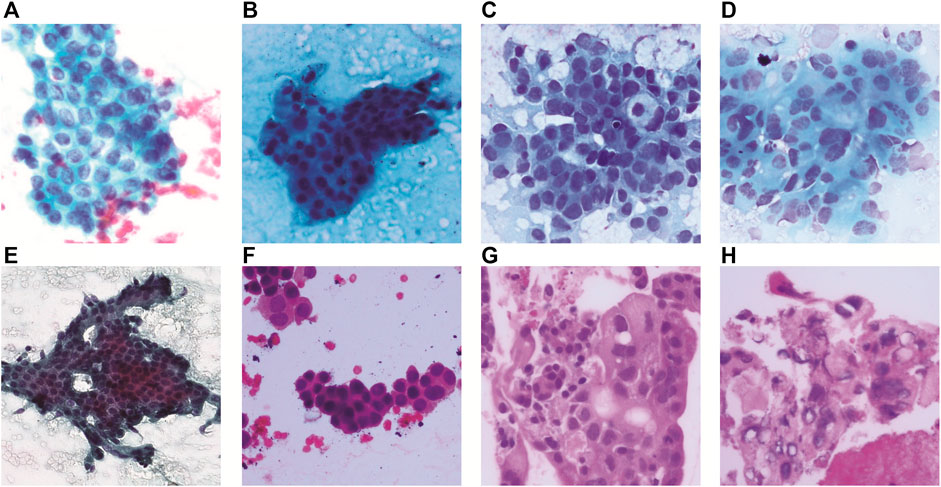
FIGURE 1. Pancreatic cancer grade and corresponding pathology image. (A) MGG: Normal, (B) MGG: Grade I, (C) MGG: Grade II, (D) MGG: Grade III, (E) H&E: Normal, (F) H&E: Grade I, (G) H&E: Grade II, and (H) H&E: Grade III.

2.2 Related Work

The advancement of the DL model enables an automated and fast discovery of many underlying features that only can be identified with exhaustive manual analysis by the medical experts. The transfer learning approach makes DL very robust to many different applications. For example, during this pandemic, DL is able to provide early detection of COVID-19–positive cases using an optimized transfer learning–based approach for quick treatment to prevent the spread (Bahgat et al., 2021). In pathological images, detection and classification of cancerous cells using DL has been widely used to extract relevant information such as morphology features on WSI to identify cancer conditions and classify them into binary or multiple classes (Bhatt et al., 2021). DL can automate many processes, but different models will perform differently with different stain types and biomarkers. DL stands out in terms of accuracy, computational efficiency, and generalizability in analyzing pathological images, specifically on segmentation (tumor region identification), detection (metastasis detection), and classification (cancer grading and patient prognosis).

Detection and assessment of pancreatic cancer is majorly done by computed tomography (CT) modality, but it is highly dependent on the radiologists’ experience. DL can help distinguish pancreatic cancer accurately on a CT scan, as studied by Liu et al. (2020) using a CNN. The challenge was to detect small tumors (less than 2 cm), and the authors proposed a patch-based detection where the optimal patch size was found to be 50 by 50 pixels or equivalent to 3.5 by 3.5 cm to detect pancreatic cancers on CT. Many other studies on pancreatic cancer grading using CT modality are available in the literature. A study by Chu et al. (2021) reviewed advanced visualization techniques for improving pancreatic cancer detection through DL. For grading the pancreatic tumor, there are two main features that have been identified from previous work: radiomics features and histogram. Radiomics features are used together with clinical features for studying specific cancer types named intraductal papillary mucinous neoplasm malignancy in pancreatic protocol CT (Hanania et al., 2016), portal venous phase CT (Permuth et al., 2016; Chakraborty et al., 2018; Attiyeh et al., 2019; Gu et al., 2019), and arterial phase CT (Gu et al., 2019). For histogram features, it was used for pancreatic neuroendocrine tumor grade and also in similar imaging (portal venous phase CT (Canellas et al., 2018), arterial phase CT (Guo et al., 2019), and both arterial and portal venous phase CT (Choi et al., 2018; D’Onofrio et al., 2019)). Histogram features are used together with texture geometrical features such as size and margin.

Grading of pancreatic cancer from pathological images has not yet been studied in DL because the cancer itself is not common (around 3% of all cancers (Society, 2021)) but deadly if misdiagnosed. This is supported by the latest review article by the British Journal of Cancer on deep learning in cancer pathology (Echle et al., 2021) covering various cancer types but not pancreatic cancer. However, we found a very recent study on detection and classification of pancreatic adenocarcinoma in WSIs using DL with EfficientNet-B1 architecture (Naito et al., 2021). This model was pre-trained using ImageNet, and the analysis for transfer learning of 372 WSIs was done using overlapping fixed-sized tiles of 512 by 512 pixels with a stride of 256 pixels. The f1-score and accuracy obtained for these endoscopic ultrasonography–guided fine-needle aspiration cytology specimens are 0.9581 and 0.9417, respectively. The work has potential as a supportive system for pathologists to diagnose difficult cases, specifically with regard to identifying the adenocarcinoma and non-adenocarcinoma tissues without grading.

For cancer grading in pathological images, the common one is using the Gleason system as the single most relevant morphological biomarker for patient stratification in prostate cancer (Echle et al., 2021). An automated Gleason grading of prostate biopsies was done by Bulten et al. (2020) on a total of 1243 annotated WSIs using an extended U-Net DL model. The model was trained on patches extracted from the internal training dataset (933 WSIs), tuned with the internal tuning dataset (100 WSIs), and tested using the internal test dataset (210 WSIs). The f1-score for the grading results of the internal test set ranges from 0.887 to 0.915 and from 0.825 to 0.898 for the external test set. A similar study was carried out by Ström et al. (2020) using two CNN ensembles, each consisting of 30 Inception V3 models pre-trained on ImageNet and adapted classification layers. The first ensemble will perform binary classification on image patches into benign or malignant, and the second ensemble will classify patches into Gleason patterns 3–5. A total of 6682 slides were digitized from needle core biopsies, and smaller patches sized 598 by 598 pixels were used at a resolution corresponding to ×10 magnification, resulting in around 5.1 million patches. The study did not measure the f1-score, but the model achieved an area under the receiver operating characteristics curve of 0.997 on the independent test dataset and 0.986 on the external validation dataset.

A research study by Karimi et al. (2020) on Gleason grading also employed a DL approach but with two augmentation techniques applied: image synthesis and image deformation. It is interesting to note that this study employed generative adversarial network architecture to synthesize superficially authentic histology images to a human observer. The image deformation methods used are jittering, elastic, and rigid deformation. Different patch sizes and massive data augmentation are used with a small amount of labeled training data. An over-sampling algorithm called the balanced batch generator is applied to address the issue of class imbalance. Three separate CNNs (CNNSmall, CNNMedium, and CNNLarge) are utilized for Gleason grading of prostate cancer of different sizes of histopathology patches. After the CNNs are trained, a logistic regression model is trained to combine the decisions of the three CNNs. The method achieved an accuracy of 0.92 in classifying cancerous patches versus benign patches and an accuracy of 0.86 in classifying low-grade from high-grade patches.

One of the promising DL networks is GoogLeNet, which has been used in WSI of kidney renal clear cell carcinoma to classify six different classes of H&E stained histology sections (normal, fat, blood, stroma, low-grade granular tumor, and high-grade clear cell carcinoma) (Khoshdeli et al., 2018). The authors employed the transfer learning method of GoogLeNet to compare with a shallow CNN (Vanilla CNN). The experiment concluded that the GoogLeNet (22 layer) network built by a repetition of the inception module can learn more diverse phenotypic signatures than the shallow network. On the other hand, the Vanilla CNN differentiated tumor samples effectively but not tumor grades. As a result, the GoogLeNet CNN gives higher performance (0.99 f1-score) than the shallow CNN (0.92 f1-score). The use of multi-task DL for colon cancer grading has been demonstrated by (Vuong et al., 2020) with a neural network consisting of DenseNet121 and two consecutive fully connected layers (classification and regression layers). Regression is applied to predict the values of a desired target quantity when the target quantity is continuous. The multitask learning neural network is evaluated on colon tissue images from six tissue microarrays and three WSIs that are stained with H&E scanned at ×40 optical magnification. Data augmentation techniques are applied on each image patch using the Aleju library (random cropping, random Gaussian blurring, random color change, random elastic transformation, and so on). The Adam optimizer is used in training using the default parameter for 100 epochs. The result showed an overall accuracy of 0.8591 with more than 98% of benign patches (Normal) being correctly classified. An accuracy of 0.832 is obtained from the Grade I, II, and III tumor patches.

From the existing studies, there are many techniques used by medical researchers to develop algorithms for diagnosing diseases. All the different algorithms and DL models show promising progress and results, but there is a lot left to do before we are able to build trustable models that are nearly as accurate as expert pathologists in diagnosing the diseases. In this study, we will contribute to the pancreatic cancer grading of pathological images for MGG and H&E stains and present it with an automated cloud-based system. The main advantage of having a cloud-based system is that the pathologist does not have to spend their time on installing or setting up the system but can easily access our portal and upload the image into the web interface. The processing will be done immediately, and results can be obtained in a short time. This pancreatic cancer grading system is yet to be found in the literature to the best of our knowledge.

3 Methodology

A computer-aided prognosis can assist the pathologists in automating the time-consuming manual identification of cancer grades from pathology images. As elaborated in the previous section, pancreatic cancer grading in pathological images has not yet been studied in computer vision. The overall methodology of this work on the pancreatic cancer grading system, named PancreaSys, is illustrated in Figure 2. The deployment of the system involved a cloud-based platform, utilizing Anvil for the graphical user interface (GUI) and Google Colab to process the algorithms. There were two major stages involved: data acquisition and DL model development. Pathology images of pancreas tissue samples were obtained from the collaborator and prepared into a dataset where each image was pre-classified by the pathologist into four classes. The dataset was then trained and evaluated using a DL network and integrated into the cloud-based system for online grading purposes. The cloud-based system allows this work to take advantage of the robust computing power available in the market and assist the pathologist to make cancer prediction and grading through the web-based application.

FIGURE 2

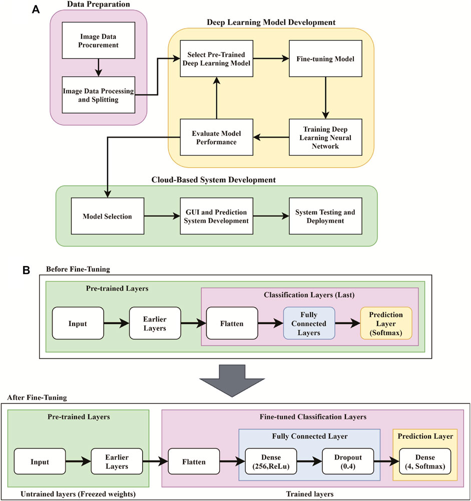
FIGURE 2. Flowchart for the development of the PancreaSys grading system. (A) Overall flowchart. (B) Pre-trained model pipeline before and after fine-tuning.

3.1 Data Acquisition

3.1.1 Pathology Image Procurement

The stain images of pancreatic tissue was obtained from our collaborator, Clinipath (Malaysia) Sdn. Bhd., and the classification of each image into subsequence grade classes was done together with a pathologist from International Medical University, Malaysia. The images were carefully organized into a folder of the class they belonged to. A total of four classes were available in the dataset, which are Normal, Grade I, Grade II, and Grade III. Each class consists of images of tissue samples with MGG and H&E stains. Labeling was done on every image for validation purposes. There are three types of high-resolution image dimensions in the dataset (1600 by 1200, 1807 by 835, and 1807 by 896), but the number of stain images in each class is unequally distributed. For example, Grade II class has the highest number of images (58) while the lowest is Normal class (20). Low number of images in each class, especially in Normal class, is not suitable for training a DL model because learning the models requires hundreds to millions of images to reduce bias in making prediction. Hence, a new dataset was prepared using the image slicing method to increase the number of images. Table 1 shows the number of HPF images, related dimensions, and sliced images procured for each grade class.

TABLE 1

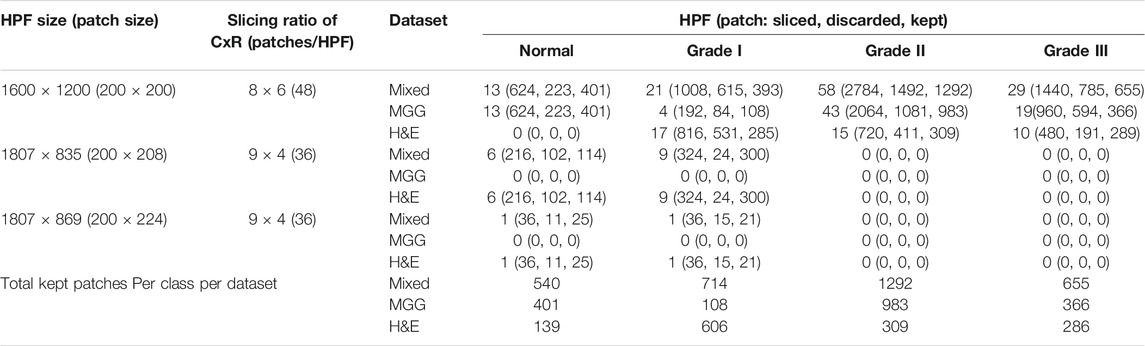
TABLE 1. Dataset distribution: number of images per class and dataset.

3.1.2 Image Slicing

Many DL models require a low dimension and square image for training and prediction. One way is to resize the original high-resolution and rectangular-shaped image into square-shaped, but this will cause loss of image information because the pixels are altered. Here, an image slicing method is used to divide the large high-resolution HPF stain images into smaller non-overlapped squared patches. The patch size will be around 200 by 200 pixels, where the exact pixel dimensions are determined using ratio equations in 1, 2. N_C and N_R are the number of rows and columns to slice, I_W and I_H are the image width and height in pixels, respectively, and P is the patch size, also in pixels. For the three types of image dimensions, the slicing ratio, output dimension, and output number of patches per image are listed in Table 1.

$N_C=I_W/P(1)$

$N_R=I_H/P(2)$

After slicing the images, many unnecessary patches appeared such as white background and non-tissue or non-cell related images that provide no value for training DL model. The first step to diagnosing is to identify the individual cells. Some of the patches contain just stain or stain of the fragmented cells. These kinds of patches were likely to introduce discrepancies and cause the model to be unable to make a good generalization. Hence, these patches were discarded from the dataset and only ones with cell clusters were kept, as illustrated in Figure 3. The slicing method will produce a larger set of images to suit the DL pre-trained model requirements. The new set of small patch images is called a “Sliced Dataset” with a total of 6468 patch images, produced from 138 original high-resolution HPF stain images, which is an increase of 468% in the number of images. 50.5% or 3267 of 6468 patch images were discarded and left with 3201 images, which will be used for building a training set and a validation set for the DL model. The detailed number of images in the Sliced dataset per image class is summarized in Table 1. Of all the images kept, 16.87% (540) were Normal, 22.31% (714) were Grade I, 40.36% (1292) were Grade II, and 20.46% (655) were Grade III. For the MGG Stain image kept, 21.58% (401) were Normal, 5.81% (108) were Grade I, 52.91% (983) were Grade II, and 19.70% (366) were Grade III. As for the H&E Stain, 10.35% (139) were Normal, 45.12% (606) were Grade I, 23% (309) were Grade II, and 21.52% (289) were Grade III. The number of images per class is still unequally distributed in this Sliced dataset, but this challenge can be mitigated by employing weighted average (WA) to evaluate the DL model, which will be explained in the CNN Deep Learning Model Development section.

FIGURE 3

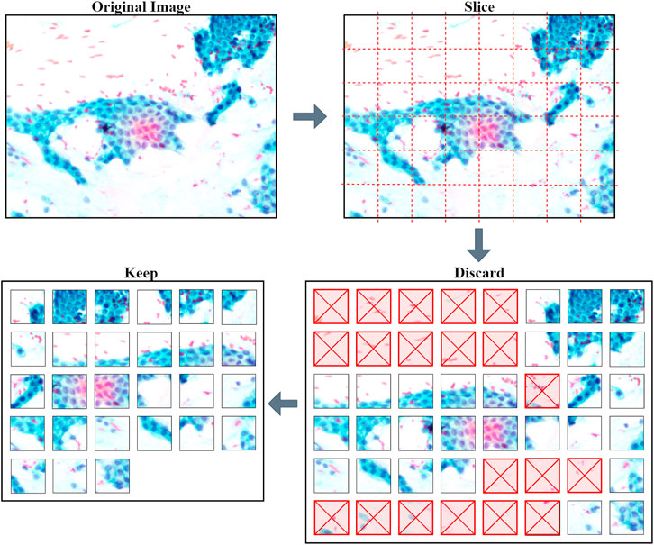
FIGURE 3. Process of slicing an image and discarding unwanted patches.

3.1.3 MGG, H&E, and Mixed Dataset

Three new datasets were created from the Sliced dataset to compare DL model performance on different stain colors of pathology images: MGG Dataset, H&E Dataset, and Mixed Dataset (with both MGG and H&E stains). The number of images is tabulated in Table 1 with the numbers of kept patches highlighted in bold font. Figure 1 shows an example of MGG stain and H&E stain pathology image.

3.1.4 Training-Validation Splitting and K-Fold Cross-Validation Set

As part of evaluating the DL model, images in a dataset are usually separated into training, validation, and testing. However, due to the limited number of images, the images in each set were split into training and validation sets only. To reduce the randomness of image selection during splitting, the K-fold CV procedure was used to allow all images in the dataset to be used for both training and validation, with the value of K = 5. Therefore, five new copies of MGG, H&E, and Mixed datasets were created and labeled accordingly (e.g., MGG Set 1 up to MGG Set 5 for MGG Dataset). These datasets are called CV sets, which were used for developing the DL model. Each set has a different set of images used for training (80%) and validation (20%). The model will be trained on five sets each where in the first iteration, the first fold is used for validation and the rest are for training. In the second iteration, the second fold is used for validation and the rest are for training. This process is repeated until each of the 5 folds is used for validation. To evaluate the performance of the model, a mean value is calculated from each training iteration.

3.1.5 Image Data Augmentation

Due to the challenge of having a small number of images in the dataset, image data augmentation is implemented to virtually expand the size of the training set. It is a process of creating a transformed version of images so there will be many variations of the same image for the model to learn during the training, but is not applied on the validation set. Data augmentation can help the model to generalize well and improve its performance on predicting the image (in validation set) as well as reducing overfitting. The transformation parameter involved is horizontal flip, vertical flip, and -90° to 90° rotation range. These procedures were done using the ImageDataGenerator() function from the Keras API Library (Keras, 2021), which creates a new batch of randomly transformed images for every training epoch. This means that in every epoch, the same number of images in the training set was used for training, but they were transformed randomly in the next subsequent epoch. Image rotations will cause an image to create a white space as it tries to fit the whole rotated image within the square perimeter. The white space is filled with symmetric padding of the image by using the “Reflect” fill mode in the ImageDataGenerator() function.

3.2 CNN Deep Learning Model Development

Deep CNN algorithms are widely used in image classification applications. The CNN algorithm for this work is to develop a model for classifying pancreatic cancer grading from pathology images. A technique called “Transfer learning” is adopted to train the small dataset. A pre-trained model with 200 convolution layers named DenseNet201 was selected from the Keras API Library to develop the best model for classifying the four grade classes of pancreatic cancer pathology images. DenseNet201 was chosen based on our preliminary study (Sehmi et al., 2021), which tested 14 powerful deep CNN models (Xception, VGG16, VGG19, ResNet50V2, ResNet101V2, ResNet152V2, Inception V3, InceptionResNetV2, MobileNetV2, DenseNet121, DenseNet169, DenseNet201, NASNetMobile, and NASNetLarge), with the top three most performed models being from the DenseNet family: DenseNet201, DenseNet169, and DenseNet121, sorted in ascending order. Huang et al. (2017) developed DenseNet, a densely connected convolutional network, inspired from ResNet (He et al., 2016) but with an improved network. In DenseNet, all previous feature maps became the input of the next layer and able to mitigate a common problem for a very deep neural network, known as the vanishing gradient. A DenseNet model is usually made from multiple dense blocks where each block is stacked with two convolution layers (1×1 and 3×3). The primary difference between DenseNet121, DenseNet169, and DenseNet201 is the number of blocks and the number of convolution layers (120, 168, and 200, respectively). DenseNet201 has the deepest network with the depth of 709, representing all layers and functions in the model such as input layer, activation layers, dropout layers, convolutional layers, pooling layers, flatten layer, and dense layers.

3.2.1 Fine-Tuning

Fine-tuning is part of the transfer learning process, done by removing the last layers such as the fully connected layer and the prediction layer and replacing it with a newer (fine-tuned) layer for our specific task. Since the pre-trained DenseNet201 model was trained on ImageNet, this experiment will take advantage of features that the model has already learned from the previous ImageNet dataset by loading the weights of ImageNet to the earlier layer. These weights were then frozen, and the layers became untrainable. Only the weights of the newly added fine-tuned layers were trained to classify the pancreatic cancer grade as shown in Figure 2B.

By referring to Figure 2B, four new layers were added as the feature extractor from pathology images. It is done after removing the last layer of the pre-trained models, and the first step is to flatten the network into a 1D array to form a fully connected layer. The fully connected layer consists of a dense layer and ReLu activation function. The dense layer is experimented with 256, 512, and 1024 nodes and is added to allow the network to learn more additional features. The weight in this layer is initially randomized with a fixed random seed value of 2020 so that the result can be reproduced. A dropout layer was added after the dense layer to regularize the network and prevent the neurons in the dense layer from converging to the same goal, which can affect the network learning ability and causes overfitting. The dropout rate is tested with 0.4, 0.6, and 0.8 to observe the effectiveness. Finally, another dense layer was added as an output layer with four nodes and SoftMax activation function to normalize the probability of prediction for four classes of pancreatic cancer grade. The output of this layer is a Python list of size 4 where each index in the list resembles the order of the class (Normal, Grade I, Grade II, and Grade III). Prediction is based on the index of the class with the highest probability.

3.2.2 Optimization and Setup

Before we begin to train the neural network, image data normalization is another step of image pre-processing which is done together with data augmentation using the ImageDataGenerator() function. It is a method where the image pixels are rescaled from a range of [0,255] to [0,1] to ensure that each input pixel has similar data distribution. A batch size of size 64 is chosen to allow the computer to train and validate 64 patch samples at the same time. An Adam optimizer with a default initial learning rate of α = 0.01 and a moment decay rate of β1 = 0.9 and β2 = 0.999 was used in this experiment to update the trainable weights of the neural network and reduce losses. Adam stands for “Adaptive Moment Estimation” where the learning rate constantly changes after every epoch. Image data normalization and the Adam optimizer have allowed faster convergence of gradient descent and achieved a faster learning rate. The loss function is calculated using categorical cross-entropy for our four classes classification task. With this setup, the model is compiled and trained for 100 epochs.

3.2.3 Performance Metrics

Confusion matrix, precision, recall, and f1-score are the metrics used for evaluating our classification model’s performance. The confusion matrix is used to evaluate the performance of the classification model. It provides a clear picture for which classes are being predicted correctly and incorrectly. It is also used to count the number of predicted samples for finding precision and recall. The normalized confusion matrix was also obtained to see the percentage of the predicted samples clearly. Precision (3) measures the ratio of the correctly predicted sample to the total predicted sample. Recall (4) measures the ratio of the correctly predicted sample to all samples in the actual class. Accuracy metric is only useful when the classes in a dataset are well balanced. Due to the challenge of having uneven class distribution, f1-score (5) is used for measuring the performance of a model instead of accuracy. F1-score measures the harmonic mean of precision and recall. It takes false positive (FP) and false negative (FN) into account while accuracy is measured when true positive (TP) and true negative (TN) are more important. Weighted average, WA (6), is computed by considering the number of images in a class of imbalanced datasets. It is calculated for precision, recall, and f1-score of each individual CV set. Since the CV set is used to evaluate the performance, the mean of all metrics such as precision, recall, and f1-score are calculated simply by averaging the WA of each individual result of the CV set. The equations are listed in 3–6.

$Precision=\frac{TP}{TP+FP}(3)$

$Recall=\frac{TP}{TP+FN}(4)$

$F1-score=2\times \frac{\left(precision\times recall\right)}{\left(precision+recall\right)}(5)$

$WA=\sum _n^{k=1}\left(P_k\times \frac{N_k}{\sum K}\right),(6)$

where

n is the total number of classes; k is the individual class; P_k is the precision, recall, or f1-score of class k; and

N is the total number of images in a class.

3.3 Cloud-Based System Development

3.3.1 System Architecture

The proposed architecture of the PancreaSys cloud-based system consists of Anvil Cloud and Google Colab platforms. The Anvil Cloud platform is used to develop the front-end of the web application using the Python language, with a GUI for the pathologist to view and interact with. It is also used to store the developed web application so the pathologist can effortlessly load the web application using a browser and not have to go through a tedious installation process on their device. The Google Cloud Platform is used to host the secondary back end of the web application system. This work uses Google Colab which is hosted on the Google Cloud Platform to develop the code for deploying the DL model and making predictions, where image processing will take place. Data transfer will happen bi-directionally between the user browser and Anvil Cloud and between Anvil Cloud and Google Cloud. Anvil Cloud acts as an intermediary between a user and the secondary back end as it will encrypt the data uploaded by the user. Data transfer will also happen when the pathologist uploads an image for prediction and configure the parameters at the web application. During the upload stage, the image will go through Anvil Cloud before arriving at Google Cloud. After prediction, the results are transferred to the pathologist via Anvil Cloud. Function calling to Anvil will happen when the pathologist interacts with the web application, such as uploading images and pressing buttons. Function calling between Anvil and Google Colab happened when the image is ready to be sent to Google Colab for prediction and return the result to Anvil to display result. The communication between Anvil and Google Colab is achieved by using Anvil Uplink API.

3.3.2 Web Application System and Design

The main purpose of building a web application is to allow a pathologist to input an image and make predictions from the image. However, the DL model was trained on roughly 200 pixels of squared patches from large images, but the pathologist needs to input an HPF because it is impractical for them to slice the image into patches. With an HPF, the prediction will not be accurate if the input image is exceptionally large and non-squared since it needs to be resized to a smaller square size and a lot of information in the image will be altered. Hence, PancreaSys is designed to help the pathologist to automatically process the large WSI, using a similar technique to that explained in the Data Preparation section. The system was designed to slice the input HPF into squared patches with a slightly modified equation from Eqs 1, 2 to find the ratio for slicing. The equations are listed in 7, 8, where h is the scaling factor. The scaling factor is introduced to allow the pathologist to choose the size of patches to see the result of prediction. In this system, the scaling factor is fixed in the program to make the system easy to use. The optimum value of h is chosen as 0.5, 1, and 1.5. Examples of output patch sizes when the input image dimension is 1600×1200 are shown in Table 2.

$N_C=\left(I_W/P\right)\times h(7)$

$N_R=\left(I_H/P\right)\times h(8)$

TABLE 2

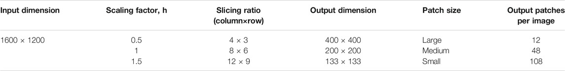
TABLE 2. Example of image slicing output with the scaling factor.

After the image was sliced in the background, PancreaSys will predict each individual patch, with a list of prediction probability for the four classes. This probability value will be referred to as the confidence value in predicting that class. The next step after making prediction is to overlay a bounding box together with the class name and its confidence level on the patches. A contrasting color of the text and bounding box was chosen to depict different classes. The color of the bounding box for each class is green (Normal), orange (Grade I), magenta (Grade II), and red (Grade III). There will be a selection for which patches will get overlayed depending on the minimum confidence threshold. If the confidence level is lower than the threshold, the patches will not be overlayed. Last, the patches will then merge back together to form a single image. At this stage, the new image is an altered version from the original image where the colored bounding box will indicate the region which the model is confident to predict. An example of the PancreaSys prediction process is shown in Figure 4.

FIGURE 4

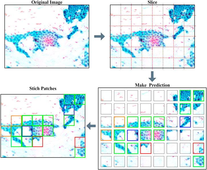
FIGURE 4. PancreaSys prediction process from MGG stain image.

When designing the GUI in Anvil for web application, several factors need to be considered to achieve good user experience. The GUI is designed to be simple and easy to use. In the main page of the web application, several important input elements in the GUI must be included, such as button to upload an image, to choose the size of patches for prediction, a slider to choose the confidence threshold, and finally, a button to begin making prediction. The main page GUI will also show basic information such as the uploaded image and other selected configuration values. After prediction, a new page showing the detailed predicted result will be loaded, together with the merged image, a histogram to show frequency of predicted classes, and also the overall predicted grade.

When the pathologist clicks the predict button, Anvil will send the uploaded image to the Google Colab back end to make prediction. The flow chart after the prediction button is pressed is shown in Figure 5. At this stage, the primary back end in the Anvil side will check if there is an input image and whether the secondary back end (Google Colab) is running. If both conditions are not satisfied, the user will see an error. Otherwise, Anvil Uplink API will send a signal to the running Google Colab program and transfer the uploaded image. Google Colab will wait until Anvil sends a signal to retrieve the image together with the configuration information. Once received, the program in Google Colab will begin slicing the image before making prediction. Then, colored bounding boxes and text will be super imposed on the patches depending on user configuration setting. The program will also count how many images were predicted in each class and then merge all patches back into a single image before sending the results to the Anvil server. Anvil will retrieve the results and choose a class with the highest frequency (majority vote) to display the overall class prediction.

FIGURE 5

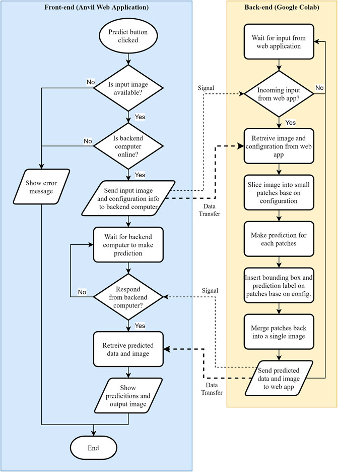
FIGURE 5. Flowchart behind the PancreaSys program when the predict button is clicked.

4 Results and Discussions

In this section, the user of PancreaSys is referred to as the pathologist, and the DenseNet201 model was trained for the system prediction using the Mixed Dataset. Figure 6 shows the PancreaSys web application GUI after the pathologist has uploaded an input image. The right pane will preview the uploaded image, and the resolution or dimension of the image is displayed in the left pane, below the upload button. There are two interactable configuration settings inside the same pane, which are the prediction patch size and prediction confidence threshold. When the pathologist chooses the prediction patch size, it will display the ratio of slicing and the number of output patches the system will predict. Figure 6B shows the result page after the pathologist pressed the “PREDICT GRADE” button. Google Colab will be running inside the Virtual Machine of Google Cloud Platform, where the DL model is deployed and the input image from the web application is processed for prediction and result.

FIGURE 6

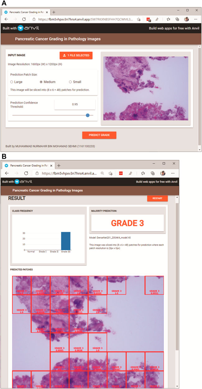
FIGURE 6. PancreaSys web application GUI: (A) main page (after an input image is uploaded); (B) result page (after prediction).

In the result page (Figure 6B), three types of results are displayed. The prominent output is an image with merged patches that shows Grade III in a red bounding box and its confidence level. There is a histogram that shows the frequency of patches predicted to the respective classes and an indicator that tells the class of the majority prediction, which in this case is Grade III. The pathologist can press the restart button to return to the main page and make a new prediction with different images or different configuration settings.

4.1 Web Configuration Settings Comparison

A sample of a full-size pathology image from the Normal class is selected to demonstrate the prediction result with different configuration settings available in the web application.

4.1.1 Comparison Between Prediction Patch Sizes

In this comparison, the confidence threshold is set at 0.95. The patch sizes of large, medium, and small will be compared. Figure 7 demonstrates the result of using the three patch sizes, respectively. The size of the patches is calculated using (Eqs 7, 8) to evenly slice the original image with different scaling factors. Table 3 shows the results from the different patch sizes. It can be seen that the prediction can still be done accurately on different patch sizes even though the model was trained on the medium-sized patch samples.

FIGURE 7

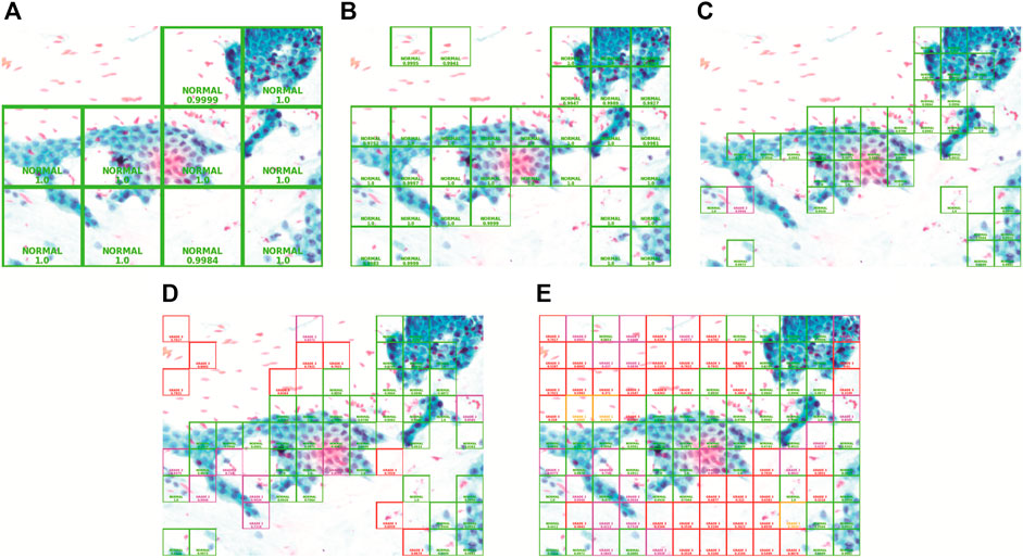
FIGURE 7. Patch size and confidence threshold (CT): (A) Large with 0.95 CT, (B) Medium with 0.95 CT, (C) Small with 0.95 CT, (D) Small with 0.7 CT, and (E) Small with 0 CT.

TABLE 3

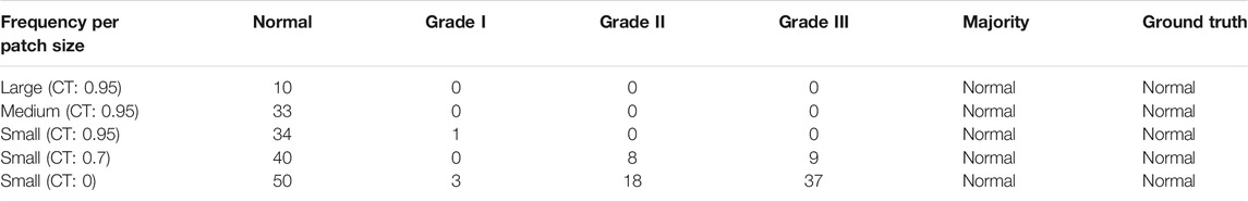
TABLE 3. Prediction results using different patch sizes and different confidence thresholds (CTs).

4.1.2 Comparison Between Different Confidence Thresholds

In this comparison, the patch size is set to “small.” The confidence threshold of 0.95, 0.7, and 0 will be analyzed. Comparing with Figures 7C–E, as the confidence threshold is reduced from 0.95 to 0.7 and 0, respectively, we can clearly see that the system will reveal more patches superimposed with colored bounding boxes in the output image with a different grade class and lower confidence level. This configuration exists for the pathologist to see in case the model could not show prediction on certain regions with high confidence. The lower confidence prediction will be inaccurate as it is also showing the prediction of the background region which does not have information about the cell tissue. Hence, it is best to keep the confidence threshold high in order to avoid the model from making inaccurate prediction on the whole full-sized image.

4.2 Data Augmentation and Effect on Model Performance

This experiment was done only with the first CV set of Mixed Dataset, to observe how data augmentation impacts a model training performance after 100 epochs. The graph result of model loss and accuracy is shown in Figure 8 for both with and without data augmentation. Looking at the graphs without data augmentation, it is evident that overfitting has occurred, where the model accuracy of the training set is much higher than that of the validation set, with the difference in model loss being −0.95 and accuracy being 14.45%. This shows that the model is doing very well on the training set but not on the validation set. The increase of the gradient in model loss indicates that the model is unable to learn enough features from the training data. With data augmentation, the graphs show consistent model loss and accuracy, where the gap is closer and validation accuracy has been improved by 2.67% and validation loss has been reduced by −0.63. The difference with training results are also lessened, −0.23 for model loss and 8.62% for model accuracy.

FIGURE 8

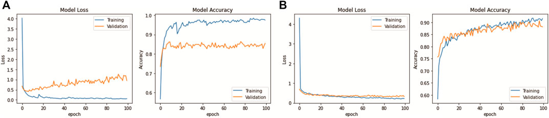
FIGURE 8. DenseNet201 model learning performance: (A) Without data augmentation. (B) With data augmentation.

4.3 Fine-Tuning Result of the Pre-Trained DenseNet201

The depth, parameters, and size of the pre-trained network model were affected, and the trainable parameters in the model network were introduced after the fine-tuning process. These trainable parameters represent the updatable weights of the model after each iteration of optimization. After fine-tuning, the DenseNet201 model produced more trainable parameters, which are 57%, 72%, and 84% of total parameters for 256, 512, and 1024 dense nodes, respectively. The number of total parameters and model size increases tremendously with the increase in dense layer nodes. Initial number of parameters before fine-tuning is 20,242,984 with a size of 80 MB. The new fine-tuned network model shows a significant increase in the total number of parameters and model size because the original pre-trained model does not have any heavy layers in their fully connected (last) layer for training ImageNet dataset whereas there are an additional two layers of depth on the fine-tuned model. The total parameters and model size after fine-tuning for 256, 512, and 1024 dense nodes are 42,407,748 (346.7 MB), 66,493,508 (622.3 MB), and 114,665,028 (1173.6 MB) for each of them.

Different dropout rates and dense layer nodes have also affected the model performance. Tested with Mixed Dataset, the mean f1-score results are illustrated in Table 4. Based on the result, the most optimum setting is found to be a dropout rate of 0.4 with 256 dense nodes, as the higher number of dense nodes will incredibly increase the model size, but with just a slight improvement of its performance. The following analysis of the DenseNet201 will be using this optimum set of parameters.

TABLE 4

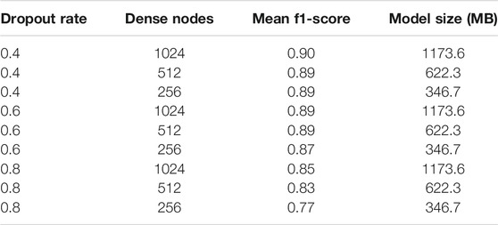
TABLE 4. Fine-tuning results: mean f1-score for different dropout rates and dense layer nodes, based on Mixed Dataset.

4.4 Analysis of Model Performance

This section presents the performance result of transfer learning for the DenseNet201 model, which was trained with three datasets: the MGG Dataset, H&E Dataset, and Mixed Dataset, with 5-fold CV. After training the DenseNet201, the evaluation was done by first obtaining the confusion matrix with a single CV set, one by one from CV1 to CV5. For each fold per dataset, both the confusion matrix and its normalized result are presented in Figure 9 (on the left and the right, respectively). Figure 10 shows the CV results for each 5-fold of all datasets.

FIGURE 9

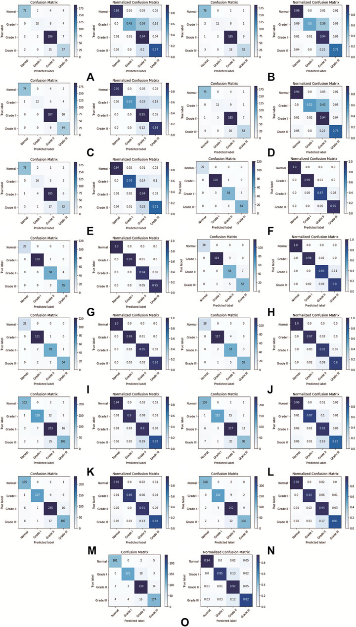
FIGURE 9. DenseNet201 model confusion matrix for each k-fold CV set: (A) Fold 1 (MGG dataset), (B) Fold 2 (MGG dataset), (C) Fold 3 (MGG dataset), (D) Fold 4 (MGG dataset), (E) Fold 5 (MGG dataset), (F) Fold 1 (H&E dataset), (G) Fold 2 (H&E dataset), (H) Fold 3 (H&E dataset), (I) Fold 4 (H&E dataset), (J) Fold 5 (H&E dataset), (K) Fold 1 (Mixed dataset), (L) Fold 2 (Mixed dataset), (M) Fold 3 (Mixed dataset), (N) Fold 4 (Mixed dataset), and (O) Fold 5 (Mixed dataset).

FIGURE 10

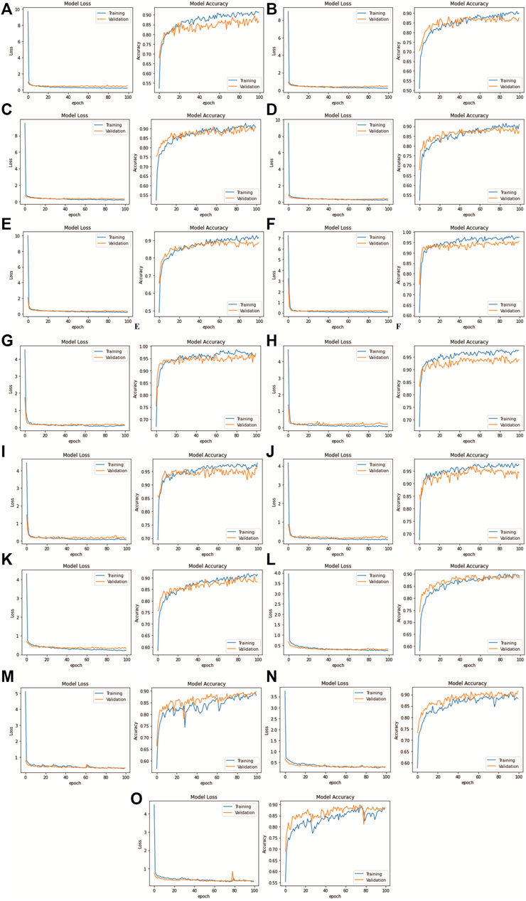
FIGURE 10. DenseNet201 model loss and accuracy with 100 epochs for each k-fold CV set: (A) Fold 1 (MGG dataset), (B) Fold 2 (MGG dataset), (C) Fold 3 (MGG dataset), (D) Fold 4 (MGG dataset), (E) Fold 5 (MGG dataset), (F) Fold 1 (H&E dataset), (G) Fold 2 (H&E dataset), (H) Fold 3 (H&E dataset), (I) Fold 4 (H&E dataset), (J) Fold 5 (H&E dataset), (K) Fold 1 (Mixed dataset), (L) Fold 2 (Mixed dataset), (M) Fold 3 (Mixed dataset), (N) Fold 4 (Mixed dataset), and (O) Fold 5 (Mixed dataset).

Further evaluation metrics such as precision, recall, and f1-score for each CV set were obtained, and the WA for each metrics was calculated. The mean performance is then calculated after training all 5-fold CV sets. The detailed performance result on individual MGG, H&E, and Mixed Dataset are presented in Table 5.

TABLE 5

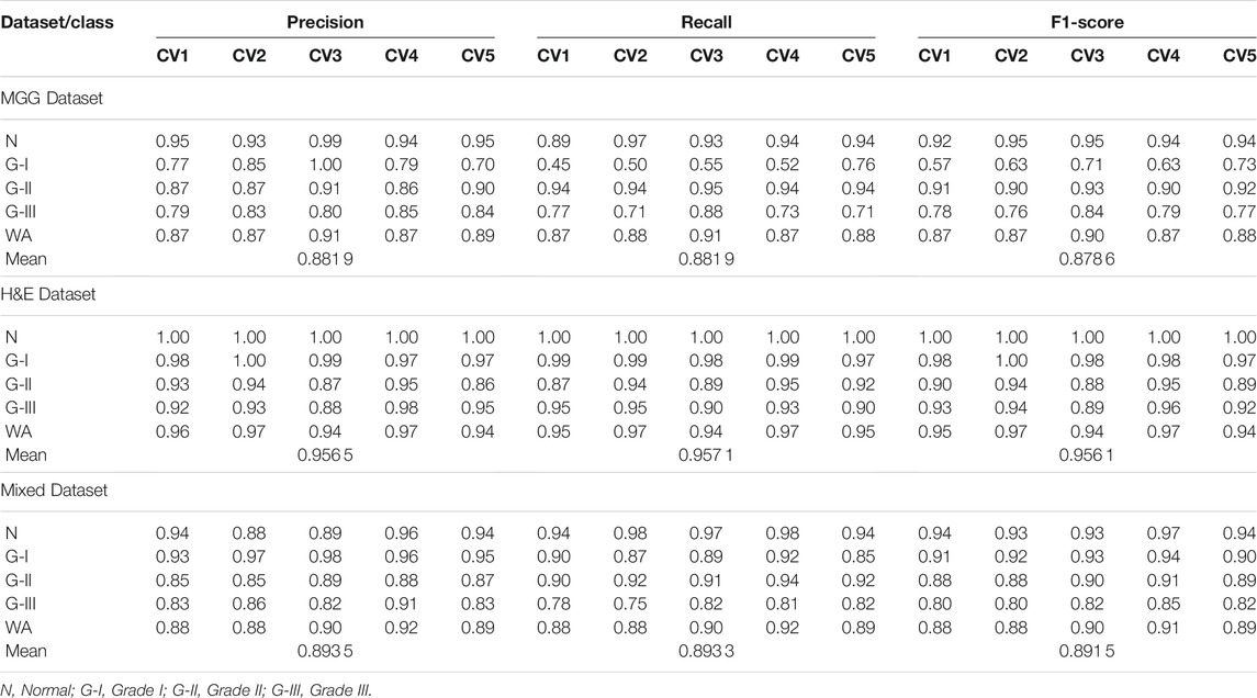
TABLE 5. Precision, recall and f1-score for 5-fold CV set of MGG, H&E, and Mixed Dataset, with WA and mean for the 5-fold CV set.

For the MGG dataset, Grade II cancer seems to be classified better than other grades, measuring recall above 0.94 for all five folds. The cause behind this is the size of Grade II images dominating 53% of the dataset. Grade I cancer has the lowest recall rate ranging from 0.45 to 0.76, due to the small amount of images, that is, 5.8% of the dataset. The WA can fairly measure the class imbalance of the MGG dataset, with a mean value of 0.88 for all precision, recall, and f1-score. In the H&E dataset, it is dominated by Grade I cancer with 45.2% images of the whole dataset, and the recall rate is 0.97–0.99. The grade with the least number of images is the Normal class with only 10.4% of the dataset, but the recall rate is perfect at 1.0 for all CV sets. The cause is due to a highly distinguishable appearance of this class (refer Figure 1E) compared to other cancer grades. Despite the imbalance class images in the H&E dataset, it can perform well in all CV sets for all performance metrics, measuring from 0.86 to 1.0, and its mean WA of 0.96. For the Mixed dataset, it is expected to perform in between the MGG and H&E datasets because it contains the two stains’ combination. The mixture, however, did not affect Grade I prediction, as it affects the MGG dataset, with the recall rate ranging from 0.87 to 0.92. The mean WA is 0.89, which is 0.01 higher than that of the MGG dataset. Since the mean WA of the H&E dataset is 0.96, this value is observed to be biased toward the MGG dataset. The reason behind this is that the MGG dataset contributed 58% of the Mixed dataset, that is, 16% more than the H&E dataset.

The results for model loss and accuracy of DenseNet201 when training each 5-fold CV set with 100 epochs are illustrated in Figure 10. The average model accuracy for the MGG dataset is 0.96 for the training set but went down to 0.88 for the validation set, where the difference is −0.08. The average model loss is 0.113 for the training set and increased from 0.301 to 0.414 for validation. This shows that images in the MGG dataset are difficult to learn, regardless of the high training accuracy. For the H&E dataset, the results are more promising, with 0.99 average model accuracy and 0.024 average model loss for the training set. For the validation set, a reduction of 0.03 is observed for average model accuracy, and an increment of 0.155 for average model loss, making them 0.96 and 0.179, respectively. Looking back at Figure 1, the differences between the images of these two datasets are visually similar to our human eyes, but somehow the DenseNet201 model performed differently when learning them. It might perform better if was trained with higher and balanced number of images in the dataset. For the training set of the Mixed dataset, the performance of average model accuracy and loss are slightly lower than that of the MGG dataset, which are 0.95 and 0.136, respectively, with a difference of −0.01 and +0.023, respectively. However, for the validation set, the Mixed dataset performs as expected, that is, in between the MGG and H&E datasets. The average model accuracy of 0.89 and 0.317 model loss is observed, still biased toward MGG dataset performance due to its higher number of images in the Mixed dataset.

For comparison with our DenseNet-based grading system, we made an analysis with other DL models in ImageNet to see how they compare with DenseNet201 in terms of performance. The models are VGG19, NASNetLarge, InceptionV3, NASNetMobile, MobileNetV2, Xception, and ResNet152V2, fed with the three datasets as trained for our system. The results of the mean f1-score are shown in Table 6, sorted in ascending order based on Mixed Dataset. Overall, all models are capable of accurately grading the H&E dataset, where they scored above 0.9 except for VGG19, just slightly lower at 0.87. This could be due to the small VGG neural network architecture and small fully connected layers making it unable to learn complex features and patterns in pathology images. The MGG dataset is a bit challenging for the models to grade because of their limited number of images, specifically for Grade I. Looking at the results for Mixed Dataset, VGG19 scored a bit low at 0.65, followed by NASNetLarge at 0.80. The Inception V3 model that was used in the study by Ström et al. (2020) for Gleason grading of prostate biopsies scored 0.83, similar to NASNetMobile, and the subsequent models’ scores show an increment of either 0.01 or 0.02. As a concluding remark, the DenseNet201 model implemented in our system still has the highest score, showing that it is the best model for grading pancreatic cancer in pathological images.

TABLE 6

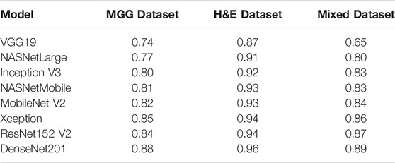
TABLE 6. Mean f1-score for other DL ImageNet models in comparison with DenseNet201, sorted in ascending order based on Mixed Dataset.

5 Conclusion

Deep learning has helped in improving the analysis and prognosis of many diseases in the medical field. This study presented a new automated cloud-based system, named PancreaSys, to assist the pathologist in classifying pancreatic cancer grades from high power field pathological images. The system comprises the DenseNet201 model for the prediction, utilizing Anvil and Google Colab platforms as its backbone. The cloud-based PancreaSys takes a high-resolution image as input using a web user interface and sliced them into smaller patches sized 200 by 200 pixels. The patches are then classified into their respective grades using DenseNet201 and are stitched back to produce one whole image before sending the final result to the pathologist. Promising f1-score measures are reported: 0.88 and 0.96 for each MGG and H&E dataset, respectively, and 0.89 for the Mixed dataset. To the best of our knowledge, no similar work on a pancreatic cancer grading system has been reported in the literature.

Improvements to the proposed system include using the state-of-the-art deep learning model, increasing the image dataset, and using color augmentation to improve the model’s learning rate on different color variation. Furthermore, a recent synthetic image generation such as a generative adversarial network can be designed to synthesize more pancreatic cancer pathology images with supervision from the experts before the training process. At this stage, this research can help to provide the pathologists a reliable diagnosis for the pancreatic cancer grade using a simple web interface, without any installation. We hope that the system will perform better with accuracy close to 1.0 in order to serve as a second opinion to the pathologist in the future.

Data Availability Statement

The datasets presented in this study can be found in online repositories. The names of the repository/repositories and accession number(s) can be found below: https://doi.org/10.17605/OSF.IO/WC4U9; https://github.com/mnmahir/FYProject-PCGIPI; https://colab.research.google.com/github/mnmahir/FYProject-PCGIPI/blob/main/System_web_app_(Backend).ipynb; https://FBM5VHPXV3N7HNS4.anvil.app/SW7RKXNBSFHH7QCWML3S7TRZ.

Ethics Statement

The studies involving human participants were reviewed and approved by IMU 434/2019: This is approval for the project under International Medical University (IMU) internal funding (2019–2020) IMU R269/2021: This is approval for the continuation of the project, under IMU external funding (2021–2022) EA2102021: This is approval from Multimedia University (MMU) for the work carried out at MMU. The project is collaborative work between MMU and IMU. The particular work reported in the article is from June 2020 to May 2021. Written informed consent for participation was not required for this study in accordance with the national legislation and the institutional requirements.

Author Contributions

MS performed the investigation, software, validation, and writing (original draft preparation). MF proposed the methodology and supervision. WA reviewed and edited the manuscript and was responsible for project administration. EC was involved in data curation and resources.

Conflict of Interest

The authors declare that the research was conducted in the absence of any commercial or financial relationships that could be construed as a potential conflict of interest.

Publisher’s Note

All claims expressed in this article are solely those of the authors and do not necessarily represent those of their affiliated organizations, or those of the publisher, the editors and the reviewers. Any product that may be evaluated in this article, or claim that may be made by its manufacturer, is not guaranteed or endorsed by the publisher.

Funding

This work was supported by the internal grants from International Medical University (IMU), Multimedia University (MMU) and IsDB-STI Transform Fund.

Acknowledgments

We would like to thank our collaborators Clinipath (Malaysia) Sdn. Bhd. for providing the image dataset and their ground truth for evaluation.

References

Attiyeh, M. A., Chakraborty, J., Gazit, L., Langdon-Embry, L., Gonen, M., Balachandran, V. P., et al. (2019). Preoperative Risk Prediction for Intraductal Papillary Mucinous Neoplasms by Quantitative Ct Image Analysis. HPB 21, 212–218. doi:10.1016/j.hpb.2018.07.016

PubMed Abstract | CrossRef Full Text | Google Scholar

Bahgat, W. M., Balaha, H. M., AbdulAzeem, Y., and Badawy, M. M. (2021). An Optimized Transfer Learning-Based Approach for Automatic Diagnosis of Covid-19 from Chest X-ray Images. PeerJ Comp. Sci. 7, e555. doi:10.7717/peerj-cs.555

CrossRef Full Text | Google Scholar

Bhatt, A. R., Ganatra, A., and Kotecha, K. (2021). Cervical Cancer Detection in Pap Smear Whole Slide Images Using Convnet with Transfer Learning and Progressive Resizing. PeerJ Comp. Sci. 7, e348. doi:10.7717/peerj-cs.348

CrossRef Full Text | Google Scholar

Bulten, W., Pinckaers, H., van Boven, H., Vink, R., de Bel, T., van Ginneken, B., et al. (2020). Automated Deep-Learning System for Gleason Grading of Prostate Cancer Using Biopsies: A Diagnostic Study. Lancet Oncol. 21, 233–241. doi:10.1016/s1470-2045(19)30739-9

PubMed Abstract | CrossRef Full Text | Google Scholar

Canellas, R., Burk, K. S., Parakh, A., and Sahani, D. V. (2018). Prediction of Pancreatic Neuroendocrine Tumor Grade Based on Ct Features and Texture Analysis. Am. J. Roentgenology 210, 341–346. doi:10.2214/ajr.17.18417

PubMed Abstract | CrossRef Full Text | Google Scholar

Chakraborty, J., Midya, A., Gazit, L., Attiyeh, M., Langdon‐Embry, L., Allen, P. J., et al. (2018). CT Radiomics to Predict High‐risk Intraductal Papillary Mucinous Neoplasms of the Pancreas. Med. Phys. 45, 5019–5029. doi:10.1002/mp.13159

PubMed Abstract | CrossRef Full Text | Google Scholar

Choi, T. W., Kim, J. H., Yu, M. H., Park, S. J., and Han, J. K. (2018). Pancreatic Neuroendocrine Tumor: Prediction of the Tumor Grade Using Ct Findings and Computerized Texture Analysis. Acta Radiol. 59, 383–392. doi:10.1177/0284185117725367

PubMed Abstract | CrossRef Full Text | Google Scholar

Chu, L. C., Park, S., Kawamoto, S., Yuille, A. L., Hruban, R. H., and Fishman, E. K. (2021). Pancreatic Cancer Imaging: A New Look at an Old Problem. Curr. Probl. Diagn. Radiol. 50, 540–550. doi:10.1067/j.cpradiol.2020.08.002

PubMed Abstract | CrossRef Full Text | Google Scholar

D'Onofrio, M., Ciaravino, V., Cardobi, N., De Robertis, R., Cingarlini, S., Landoni, L., et al. (2019). Ct Enhancement and 3d Texture Analysis of Pancreatic Neuroendocrine Neoplasms. Sci. Rep. 9, 2176–2178. doi:10.1038/s41598-018-38459-6

PubMed Abstract | CrossRef Full Text | Google Scholar

Echle, A., Rindtorff, N. T., Brinker, T. J., Luedde, T., Pearson, A. T., and Kather, J. N. (2021). Deep Learning in Cancer Pathology: A New Generation of Clinical Biomarkers. Br. J. Cancer 124, 686–696. doi:10.1038/s41416-020-01122-x

CrossRef Full Text | Google Scholar

Gu, D., Hu, Y., Ding, H., Wei, J., Chen, K., Liu, H., et al. (2019). Ct Radiomics May Predict the Grade of Pancreatic Neuroendocrine Tumors: A Multicenter Study. Eur. Radiol. 29, 6880–6890. doi:10.1007/s00330-019-06176-x

PubMed Abstract | CrossRef Full Text | Google Scholar

Guo, C., Zhuge, X., Wang, Z., Wang, Q., Sun, K., Feng, Z., et al. (2019). Textural Analysis on Contrast-Enhanced Ct in Pancreatic Neuroendocrine Neoplasms: Association with Who Grade. Abdom. Radiol. 44, 576–585. doi:10.1007/s00261-018-1763-1

PubMed Abstract | CrossRef Full Text | Google Scholar

Hanania, A. N., Bantis, L. E., Feng, Z., Wang, H., Tamm, E. P., Katz, M. H., et al. (2016). Quantitative Imaging to Evaluate Malignant Potential of Ipmns. Oncotarget 7, 85776–85784. doi:10.18632/oncotarget.11769

PubMed Abstract | CrossRef Full Text | Google Scholar

He, K., Zhang, X., Ren, S., and Sun, J. (2016). “Deep Residual Learning for Image Recognition,” in Proceedings of the IEEE Computer Society Conference on Computer Vision and Pattern Recognition, Las Vegas, NV, June 27–30, 2016. doi:10.1109/CVPR.2016.90

CrossRef Full Text | Google Scholar

Huang, G., Liu, Z., Van Der Maaten, L., and Weinberger, K. Q. (2017). “Densely Connected Convolutional Networks,” in Proceedings - 30th IEEE Conference on Computer Vision and Pattern Recognition, CVPR 2017, Honolulu, HI, July 21–26, 2017, 2261–2269. doi:10.1109/CVPR.2017.243

CrossRef Full Text | Google Scholar

Karimi, D., Nir, G., Fazli, L., Black, P. C., Goldenberg, L., and Salcudean, S. E. (2020). Deep Learning-Based Gleason Grading of Prostate Cancer from Histopathology Images-Role of Multiscale Decision Aggregation and Data Augmentation. IEEE J. Biomed. Health Inform. 24, 1413–1426. doi:10.1109/JBHI.2019.2944643

PubMed Abstract | CrossRef Full Text | Google Scholar

Keras (2021). Keras Applications. Available at: https://keras.io/api/applications/ (Accessed December 15, 2020)

Google Scholar

Khoshdeli, M., Borowsky, A., and Parvin, B. (2018). “Deep Learning Models Differentiate Tumor Grades from H&E Stained Histology Sections,” in Proceedings of the Annual International Conference of the IEEE Engineering in Medicine and Biology Society, EMBS, Honolulu, HI, July 18–21, 2018. doi:10.1109/EMBC.2018.8512357

CrossRef Full Text | Google Scholar

Liu, K.-L., Wu, T., Chen, P.-T., Tsai, Y. M., Roth, H., Wu, M.-S., et al. (2020). Deep Learning to Distinguish Pancreatic Cancer Tissue from Non-cancerous Pancreatic Tissue: A Retrospective Study with Cross-Racial External Validation. The Lancet Digital Health 2, e303–e313. doi:10.1016/S2589-7500(20)30078-9

PubMed Abstract | CrossRef Full Text | Google Scholar

McGuigan, A., Kelly, P., Turkington, R. C., Jones, C., Coleman, H. G., and McCain, R. S. (2018). Pancreatic Cancer: A Review of Clinical Diagnosis, Epidemiology, Treatment and Outcomes. Wjg 24, 4846–4861. doi:10.3748/wjg.v24.i43.4846

PubMed Abstract | CrossRef Full Text | Google Scholar

Naito, Y., Tsuneki, M., Fukushima, N., Koga, Y., Higashi, M., Notohara, K., et al. (2021). A Deep Learning Model to Detect Pancreatic Ductal Adenocarcinoma on Endoscopic Ultrasound-Guided fine-needle Biopsy. Sci. Rep. 11, 8454–8458. doi:10.1038/s41598-021-87748-0

PubMed Abstract | CrossRef Full Text | Google Scholar

Nam, S., Chong, Y., Jung, C. K., Kwak, T.-Y., Lee, J. Y., Park, J., et al. (2020). Introduction to Digital Pathology and Computer-Aided Pathology. J. Pathol. Transl Med. 54, 125–134. doi:10.4132/jptm.2019.12.31

CrossRef Full Text | Google Scholar

Pereira, S. P., Oldfield, L., Ney, A., Hart, P. A., Keane, M. G., Pandol, S. J., et al. (2020). Early Detection of Pancreatic Cancer. Lancet Gastroenterol. Hepatol. 5, 698–710. doi:10.1016/S2468-1253(19)30416-9

PubMed Abstract | CrossRef Full Text | Google Scholar

Permuth, J. B., Choi, J., Balarunathan, Y., Kim, J., Chen, D.-T., Chen, L., et al. (2016). Combining Radiomic Features with a Mirna Classifier May Improve Prediction of Malignant Pathology for Pancreatic Intraductal Papillary Mucinous Neoplasms. Oncotarget 7, 85785–85797. doi:10.18632/oncotarget.11768

PubMed Abstract | CrossRef Full Text | Google Scholar

Sehmi, M. N. M., Fauzi, M. F. A., Ahmad, W. S. H. M. W., and Ling, E. C. W. (2021). “Pancreatic Cancer Grading in Pathology Images,” in Multimedia University Engineering Conference (MECON 2021).

Google Scholar

Society, A. C. (2021), Cyberjaya, Malaysia, June 21–23, 2021. [Dataset]

Ström, P., Kartasalo, K., Olsson, H., Solorzano, L., Delahunt, B., Berney, D. M., et al. (2020). Artificial Intelligence for Diagnosis and Grading of Prostate Cancer in Biopsies: A Population-Based, Diagnostic Study. Lancet Oncol. 21, 222–232. doi:10.1016/S1470-2045(19)30738-7

PubMed Abstract | CrossRef Full Text | Google Scholar

Vuong, T. L. T., Lee, D., Kwak, J. T., and Kim, K. (2020). “Multi-task Deep Learning for colon Cancer Grading,” in 2020 International Conference on Electronics, Information, and Communication, ICEIC 2020, Barcelona, Spain, January 19–22, 2020. doi:10.1109/ICEIC49074.2020.9051305

PubMed Abstract | CrossRef Full Text | Google Scholar

Wasif, N., Ko, C. Y., Farrell, J., Wainberg, Z., Hines, O. J., Reber, H., et al. (2010). Impact of Tumor Grade on Prognosis in Pancreatic Cancer: Should We Include Grade in AJCC Staging? Ann. Surg. Oncol. 17, 2312–2320. doi:10.1245/s10434-010-1071-7

PubMed Abstract | CrossRef Full Text | Google Scholar