 Spilios Evmorfos1†
 Dionysios Kalogerias
 Athina Petropulu
- 1Electrical and Computer Engineering, Rutgers, The State University of New Jersey, New Brunswick, NJ, United States
- 2Electrical Engineering, Yale University, New Haven, CT, United States
We consider the problem of joint beamforming and discrete motion control for mobile relaying networks in dynamic channel environments. We assume a single source-destination communication pair. We adopt a general time slotted approach where, during each slot, every relay implements optimal beamforming and estimates its optimal position for the subsequent slot. We assume that the relays move in a 2D compact square region that has been discretized into a fine grid. The goal is to derive discrete motion policies for the relays, in an adaptive fashion, so that they accommodate the dynamic changes of the channel and, therefore, maximize the Signal-to-Interference + Noise Ratio (SINR) at the destination. We present two different approaches for constructing the motion policies. The first approach assumes that the channel evolves as a Gaussian process and exhibits correlation with respect to both time and space. A stochastic programming method is proposed for estimating the relay positions (and the beamforming weights) based on causal information. The stochastic program is equivalent to a set of simple subproblems and the exact evaluation of the objective of each subproblem is impossible. To tackle this we propose a surrogate of the original subproblem that pertains to the Sample Average Approximation method. We denote this approach as model-based because it adopts the assumption that the underlying correlation structure of the channels is completely known. The second method is denoted as model-free, because it adopts no assumption for the channel statistics. For the scope of this approach, we set the problem of discrete relay motion control in a dynamic programming framework. Finally we employ deep Q learning to derive the motion policies. We provide implementation details that are crucial for achieving good performance in terms of the collective SINR at the destination.
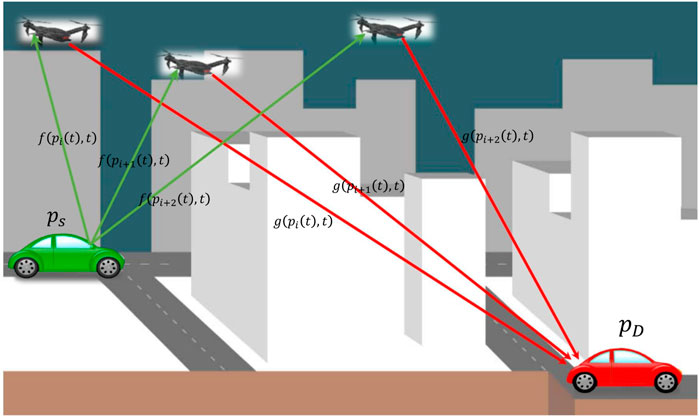
GRAPHICAL ABSTRACT
1 Introduction
In distributed relay beamforming networks, spatially distributed relays synergistically support the communication between a source and a destination (Havary-Nassab et al., 2008a; Li et al., 2011; Liu and Petropulu, 2011). The concepts of distributed beamforming hold the promise of extending the communication range and of minimizing the transmit power that is being wasted by being scattered to unwanted directions (Barriac et al., 2004).
Intelligent node mobility has been studied as a means of improving the Quality-of-Service (QoS) in communications. In (Chatzipanagiotis et al., 2014), the interplay of relay motion control and optimal transmit beamforming is considered with the goal of minimizing the relay transmit power, subject to a QoS-related constraint. In (Kalogerias et al., 2013), optimal relay positioning in the presence of an eavesdropper is considered, aiming to maximize the secrecy rate. In the context of communication-aware robotics, motion has been controlled with the goal of maintaining in-network connectivity (Yan and Mostofi, 2012; Yan and Mostofi, 2013; Muralidharan and Mostofi, 2017).
In this work, we examine the problem of optimizing the sequence of relay positions (relay trajectory) and the beamforming weights so that some SINR-based metric is maximized at the destination. The assumption that we adopt is that the channel evolves as a stochastic process that exhibits spatiotemporal correlations. Intrinsically, optimal relay positioning requires the knowledge of the Channel State Information (CSI) in all candidate positions at a future time instance. This is almost impossible to achieve since the channel varies with respect to time and space. Nonetheless, since the channel exhibits spatiotemporal correlations (induced by the shadowing propagation effect (Goldsmith, 2005; MacCartney et al., 2013) that is prominent in urban environments), it can be, explicitly or implicitly, predicted. We follow two different directions, when it comes to the discrete relay motion control.
The first direction (Kalogerias and Petropulu, 2018; Kalogerias and Petropulu, 2016) (we call it model-based) pertains to the formulation of a stochastic program that computes the beamforming weights and the subsequent relay positions, so that some SINR-based metric at the destination is maximized, subject to a total relay power budget, assuming the availability of causal CSI information. This 2-stage problem is equivalent to a set of 2-stage subproblems that can be solved in distributed fashion, one by each relay. The objective of each subproblem is impossible to be analytically evaluated, so an efficient approximation is proposed. This approximation acts as a surrogate to the initial objective. The surrogate relies on the Sample Average Approximation (SAA) (Shapiro et al., 2009). The term “model-based” is not to be confused with model-based reinforcement learning. We just use it because this method (or direction rather) assumes complete knowledge of the underlying correlation structure of the channels, so it is helpful formalism to distinguish this method from the second approach that makes no particular assumption for the channel statistics.
The second direction (Evmorfos et al., 2021a; Evmorfos et al., 2021b; Evmorfos et al., 2022) tackles the problem of discrete relay motion control from a dynamic programming viewpoint. We formulate the Markov Decision Process (MDP), that is induced by the problem of controlling the motion. Finally, we employ deep Q learning (Mnih et al., 2015) to find relay motion policies that maximize the sum of SINRs at the destination over time. We propose a pipeline for adapting deep Q learning for the problem at hand. We experimentally show that Multilayer Perceptron Neural Networks (MLPs) cannot capture high frequency components in natural signals (in low-dimensional domains). This phenomenon, referred to as “Spectral Bias” (Jacot et al., 2018) has been observed in several contexts, and also arises as an issue in the adaptation of deep Q learning for the relay motion control. We present an approach to tackle spectral bias, by parameterizing the Q function with a Sinusoidal Representation Network (SIREN) (Sitzmann et al., 2020).
Our intentions for this work lie in two directions. First, we attempt to compare two methods for relay motion control in urban communication environments. The two methods constitute two different viewpoints in terms of tackling the problem. The first method assumes complete knowledge on the underlying statistics of the channels (model-based) Kalogerias and Petropulu, (2018). The second method is completely model-free in the sense that it drops all assumptions for knowledge of the channel statistics and employs deep reinforcement learning to control the relay motion Evmorfos et al. (2022). In addition to the head-to-head comparison, we propose a slight variation of the model-free method that deviates from the one in Evmorfos et al. (2022) by augmenting the state with the addition of the timestep as an extra feature. This variation is more robust than the previous one, especially when the shadowing component of the urban environment is particularly strong.
Notation: We denote the matrices and vectors by bold uppercase and bold lowercase letters, respectively. The operators
2 Problem Formulation
2.1 System Model
Consider a scenario where source
Source
where fr denotes the flat fading channel from
Each relay operates in an Amplify-and-Forward (AF) fashion, i.e., it transmits received signal, xr(t), multiplied by weight
where gr denotes the flat fading channel from relay Rr to destination
where ysignal(t) is the received signal component and
In the following, we will use the vector
2.2 Channel Model
The channel evolves in time and space and can be described in statistical terms. In particular, during time slot t, the channel between the source and a relay positioned at
where
The logarithm of the squared channel magnitude of Eq. 1 converts the multiplicative channel model into an additive one, i.e.,
with
where η2 is the shadowing power, and
The multipath fading component,
where
with c1 denoting the correlation distance, and c2 the correlation time. Similar correlations hold for similarly
Further,
where
and c3 denoting the correlation distance of the source-destination channel (Kalogerias and Petropulu, 2018).
2.3 Joint Scheduling of Communications and Controls
Let us assume the same carrier for all communication tasks, and employ a basic joint communication/decision making TDMA-like protocol. At each time slot
1. The source broadcasts a pilot signal to all relays, based on which the relays estimate their channels to the source.
2. The destination also broadcasts pilots, which the relays use to estimate their channels relative to the destination.
3. Then, based on the estimated channels, the relays beamform in AF mode. Here we assume perfect CSI estimation.
4. Based on the CSI that has been received up to that point, a decision is made on where the relays need to go to, and relay motion controllers are determined to steer the relays to those positions.
The above steps are repeated for NT time slots. Let us assume that the relays pass their estimated CSI to the destination via a dedicated low-rate channel. This simplifies information decoding at the destination (Gao et al., 2008; Proakis and Salehi, 2008).
Concerning relay motion, we assume that the relays obey the differential equation (Kalogerias and Petropulu, 2018)
where
with
To determine the relay motion controller
Based on the above, the motion control problem can be formulated in terms of specifying the relay positions at the next time slot, given the relay positions at the current time slot and the estimated CSI. We assume here for simplicity that there exists some path planning and collision avoidance mechanism, the derivation of which is out of the scope of this paper.
For simplicity and tractability, we are assuming that the channel is the same for every position within each grid cell, and for the duration of each time slot. In other words, we are essentially adopting a time-space block fading model, at least for motion control purposes. This is a valid approximation of reality as the grid cell size and the time slot duration become smaller, at the expense of more stringent resource constraints at the relays, and faster channel sensing capability. Under this setting, communication and relay control can indeed happen simultaneously within each time slot, with the understanding that at the start of the next time slot, each relay must have completed their motion (starting at the previous time slot–also see our discussion earlier in this section–). In this way, our approach is valid in a practical setting where communication needs to be continuous and uninterrupted.
Additionally, we are assuming that the relays move sufficiently slowly, such that the local spatial and temporal changes of the wireless channel due to relay motion itself are negligible, e.g., Doppler shift effects. Then, spatial and temporal variations in channel quality are only due to changes in the physical environment, which happen at a much slower rate than that of actual communication. Note that this is a standard requirement for achieving a high communication rate, whatsoever.
We see that there is a natural interplay between relay velocity and the relative rate of change of the communication channel Kalogerias and Petropulu (2018). The challenge here is to identify a fair tradeoff between a reasonable relay velocity, grid size and a time slot, which would enable simultaneously faithful channel prediction and feasible and effective motion control (adherring to potential relay motion constraints). The width of the communication time slot depends on the spatial characteristics of the terrain, which varies with each application. This also determines the sampling rate employed for identifying the parameters of the adopted channel model. In theory, for a given relay velocity, the relays could move to any position up to which the channel remains correlated. However, as the per time slot rate of communications depends on the relay velocity (characterizing system throughput), the relays should move to much smaller distances within the slot.
In the following we use
2.4 Spatially Controlled SINR Maximization at the Destination
Next, we present the first stage of the 2-stage generic formulation. The 2-stage approach optimizes network QoS by optimally selecting beamforming weights and relay positions, on a per time slot basis. In this subsection, we focus on the calculation of the beamforming weights. The calculation of the weights at each step remains the same both for the stochastic programming (model-based) method and the dynamic programming (model-free) method.
Optimization of Beamforming Weights: At time slot
where
where, dropping the dependence on
The optimization problem of Eq. 3 is always feasible, as long as Pc is nonnegative, and the optimal value of Eq. 3 can be expressed in closed form as (Havary-Nassab et al., 2008b)
for all
The above analytical expression of the optimal value Vt in terms of relay positions and their corresponding channel magnitudes will be key in our subsequent development.
3 Stochastic Programming for Myopic Relay Control
During time slot t − 1, we need to determine the relay positions for time slot t, so that we achieve the maximum Vt. However, at time slot t − 1, we only know
Since deterministic optimization of Vt with respect to
to be solved at time slot
The map
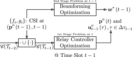
FIGURE 1. 2-Stage optimization of beamforming weights and relay motion controls. The variable
As compared to traditional AF beamforming for a static case, our spatially controlled system described above, uses the same CSI as in the stationary case, to predict the optimal beamforming performance in its vicinity in the MMSE sense, and moves to the optimally selected location. The prediction here relies on the aforementioned spatiotemporal channel model. Of course, this requires a sufficiently slowly varying channel relatively to relay motion, which can be guaranteed if the motion is constrained within small steps.
3.1 Motion Policies & the Interchangeability Principle
To assist in the process of understanding the techniques to solve Eq. 4, we make note of an important variational property of Eq. 4, related to the long-term performance of the proposed spatially controlled beamforming system. Our discussion pertains to the employment of the so-called Interchangeability Principle (IP) (Bertsekas and Shreve, 1978; Bertsekas, 1995; Rockafellar and Wets, 2004; Shapiro et al., 2009; Kalogerias and Petropulu, 2017), also known as the Fundamental Lemma of Stochastic Control (FLSC) (Astrom, 1970; Speyer and Chung, 2008) Kalogerias and Petropulu, (2018). The IP refers conditions that allow the interchange of expectation and maximization or minimization in general stochastic programs.
A version of the IP for the first-stage problem of (4) is established in (Kalogerias and Petropulu, 2017) Specifically, the IP implies that (4) is exchangeable by the variational problem (Kalogerias and Petropulu, 2017)
to be solved at each
for all
3.2 Near-Optimal Beamformer Motion Control
One can readily observe that the problem of (4) is separable. Given that, for each
at each
However, the objective of problem Eq. 11 is impossible to obtain analytically, and it is necessary to resort to some well behaved and computationally efficient surrogates. Next, we present a near-optimal such approach. The said approach relies on global function approximation techniques, and achieves excellent empirical performance.
The proposed approximation to the stochastic program (11) will be based on the following technical, though simple, result.
Lemma 1 (Big Expectations) (Kalogerias and Petropulu, 2018) Under the assumptions of the wireless channel model, it is true that, at any
for all
with m1:t−1, μ1:t−1,
at any
The detailed description of the proposed technique for efficiently approximating our base problem (11) now follows.
Sample Average Approximation (SAA): This is a direct Monte Carlo approach, where, at worst, existence of a sampling, or pseudosampling mechanism at each relay is assumed, capable of generating samples from a bivariate Gaussian measure. We may then observe that the objective of Eq. 11 can be represented, for all
for any choice of
for all
for all
Now, for each relay
the SAA of our initial problem Eq. 11 is formulated as
at relay
On the downside, computing the objective of the SAA problem Eq. 12 assumes availability of Monte Carlo samples, which could be restrictive in certain scenarios. Nevertheless, assuming mutual independence of the sequences
We denote this approach as SAA for the rest of the paper. The control flow of the SAA is presented in Algorithm 1.
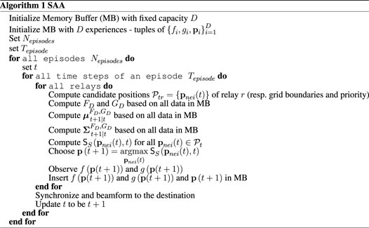
Algorithm 1. SAA
4 Deep Reinforcement Learning for Adaptive Discrete Relay Motion Control
4.1 Dynamic Programming for Relay Motion Control
The previously mentioned approach tackles the problem of relay motion control from a myopic perspective in the sense that the stochastic program is formulated so as to select the relay positions for the subsequent time slot with the goal of maximizing the collective SINR at the destination only for that particular slot.
The employment of reinforcement learning for the problem of discrete relay motion control entails that we reformulate the problem as a dynamic program. In this set up we want, at time slot t − 1, to derive a motion policy (a methodology for choosing the relays’ displacement) so as to maximize the discounted sum of VIs (in expectation) from the subsequent time step t to the infinite horizon.
To formally pose that program we need to introduce a Markov Decision Process (MDP). The MDP is a tuple defined as
The formulation of the dynamic program is as follows:
If γ is a discount factor, we can formulate the infinite horizon relay control problem as:
where u(t) is the control at time t (essentially determining the relay displacement), and the driving noise W(t) is distributed as
Now, either the above problem defines a MDP or POMDP is dependent on the history
On the other hand, if
4.2 Deep Q Learning for Discrete Relay Motion Control
The employment of deep Q learning for relay motion control expels the need for making particular assumption for the underlying correlation structure of the channels.
Taking into account the (12) one can infer that we can construct a single policy that is learned by the collective experience of all the agents/relays and it constitutes the single policy that the movement of all relays strictly adhere to. In that spirit, we instantiate one neural network to parameterize the state-action value function (Q) and it is being trained on the experiences of all the relay. The motion policy is ϵ-greedy with respect to the estimation of the Q function.
Initially, we adopt the deep Q learning algorithm as described in (Mnih et al., 2015) and illustrated in Figure 2. Even though, as we pointed out in the previous subsection, the state of the MDP is the concatenation of the relay position p = s and the channels f (p, t) and g (p, t), we follow a slightly different approach in the adoption of deep Q learning. In particular, the input to the neural network is the concatenation of the position p = [x, y] and the time step t. We should note at this point that augmenting the neural network input with the timestamp of the transition is a differentiation between the algorithm presented in this current work and the solution proposed in Evmorfos et al. (2022). This alternative, even though does not affect the implementation much, provides measurable improvements in cases where the power of the shadowing is strong. The reward r is the contribution of the relay to the SINR at the destination during the respective time step (VI). At each time slot the relay selects an action
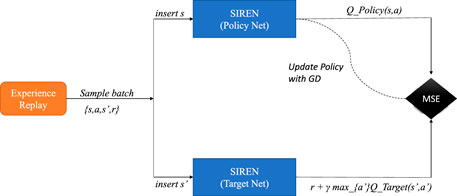
FIGURE 2. Figure for visualizing the Pipeline of the deep Q learning with SIRENs approach.
In general, Q learning with rich function approximators such as neural networks requires some heuristics for stability. The first such heuristic is the Experience Replay (Mnih et al., 2015). Each tuple of experience for a relay, namely
The second heuristic is the Target Network (Mnih et al., 2015). The Target Network (Qtarget (s′, a′; θ−)) provides the estimation for the targets (labels) for the updates of the Policy Network (Qpolicy (s′, a′; θ+)), i.e., the network used for estimating the Q function. The two networks share (typically) the same architecture. We do not update the Target Network’s weights with any optimization scheme, but, after a predefined number of training steps, the weights of the Policy Network are copied to the Target Network. This provides stationary targets for the weight updates and brings the task of the Q function approximation closer to a supervised learning paradigm.
Therefore, at each update step we sample a batch of experiences from the Experience Replay and use the batch to perform gradient descent on the loss:
At each step, the Policy Network’s weights are updated according to:
where,
The parameter λ is the learning rate. The parameter γ is a scalar called the discount factor and γin (0, 1). The choice for the discount factor pertains to a trade off between the importance assigned to long term rewards and the importance assigned to short term rewards. The parameters a,
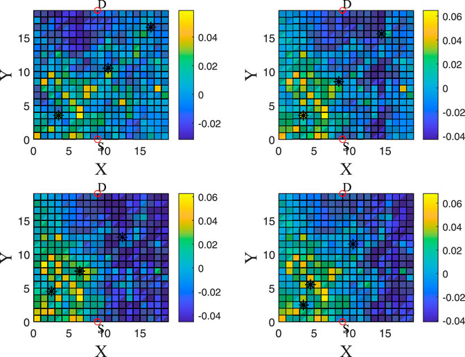
FIGURE 3. This is a heatmap for visualizing a trajectory of the relays. We can see the VI for all grid cells for four different time steps (each time step has a 2-time-slot difference with the previous and the next). One can see the positions of the relays for every time slot. The relays are moving towards better and better positions (larger VIs).
When the relays move (the do not stay in the same grid cell for two consecutive slots), they require additional energy consumption. i some cases though, the diplacement to a neighboring grid cell does not correspond to significant improvement in terms of the cumulative SINR at the destination. Therefore, to account for the energy used for the application, we choose to not perform the ϵ-greedy policy directly on the estimates Qpolicy (s, a; θ+) of the Q function, but we decrease the estimates for all actions a, except for the action
4.3 Sinusoidal Representation Networks for Q Function Parameterization
There have been many recent works which convincingly claim that coordinate-based Multilayer Perceptron Neural Networks (MLPs), i.e., MLPs that map a vector of coordinates to a low-dimensional natural signal, fail to learn high frequency components of the said signal. This constitutes a phenomenon that is called the spectral bias in machine learning literature (Jacot et al., 2018; Cao et al., 2019). The work in (Sitzmann et al., 2020) examines the amelioration of spectral bias for MLPs. The inadequacy of MLPs for such inductive biases is bypassed by introducing a variation of the conventional MLP architecture with sinusoid (sin (⋅)) as activation function between layers. Tis MLP alternative was termed Sinusoidal Representation Networks (SIRENs), and was shown, both theoretically and experimentally, to effectively tackle the spectral bias.
The sinusoid is a periodic function which is quite atypical as a choice for activation function in neural networks. The authors in (Sitzmann et al., 2020) propose the employment of weight initialization framework so that the distribution of activations is retained during training and convergence is achieved without the network oscillating.
In particular, if we assume an intermediate layer of the neural network with input
When we adopt the deep Q learning approach for discrete relay motion control, we basically train a neural network (MLP) to learn a low-dimensional natural signal from coordinates, namely the state-action value function Q (s, a). The Q function, Q (s, a), represents the sum of SINR at the destination that the relays are expected to achieve for an infinite time horizon, starting from the respective position s and performing action a. The Policy Network, being a coordinate MLP may not be able to converge for the high frequency components of the underlying Q function that arise from the fact that the channels exhibit very abrupt spatiotemporal variations.
Therefore we propose that both the Policy and the Target Networks are SIRENs. The control flow of the algorithm we propose is given in Algorithm 2. We denote this as DQL-SIREN, which stands for Deep Q Learning with Sinusoidal Representation Networks.
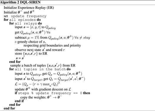
Algorithm 2. DQL-SIREN
5 Simulations
We test our proposed schemes by simulating a 20, ×, 20 m grid. All the grid cells are 1m × 1m. The number of agents/relays that assist the single source destination communication pair is R = 3. For every time slot the position of each relay is constrained within the boundaries of the gridded region and also constrained to adhere to a predetermined relay movement priority. Only one relay can occupy a grid cell per time slot. The center of the relay/agent and the center of the respective grid cell coincide.
When it comes to the shadowing part of our assumed channel model, we define a threshold θ which quantifies the distance in time and space where the shadowing component is important and can be taken into account for the construction of the motion policy. We assume that the shadowing power η2 = 15 and the autocorrelation distance is c1 = 10m and the autocorrelation time is c2 = 20sec. The variances of noises at the relays and destination are fixed as
Each one of the relays can move 1 grid cell/time slot and the size of each cell is 1m × 1m (as mentioned before). The time slot length is set to be 0.6sec. Therefore the calculation of the channel and the decision of the movement for each relay should take up an amount of time that is strictly less than the duration of the time interval.
5.1 Specifications for the DQL-SIREN and the SAA
Regarding the DQL-SIREN, we employ SIRENs for both the Policy and the Target Networks. Each SIREN is comprised by three dense layers (350 neurons for each layer) and the learning rate is 1e − 4.
The Experience Replay size is 3,000 tuples and we begin every experiment with 300 transitions derived by a completely random policy before the start of training for all the deep Q learning approaches. The ϵ of the ϵ-greedy policy is initialized to be 1 but it is steadily decreased until it gets to 0.1 This is a very typical regime in RL. It is a very simple way to handle the dilemma between exploration and exploitation in RL, where we begin by giving emphasis to exploration first and then gradually exploration is traded for exploitation. We copy the weights of the Policy Network to the weights of the Target Network every 100 steps of training. The batch size is chosen to be 128 (even though the methods work reliably for different batch sizes ranging from 64 to 512) and the discount factor γ is chosen to be 0.99. We want to mention that small values for γ translate to a more myopic agent (an agent that assigns significance to short term rewards at the expense of long term/delayed rewards). On the other hand, values of γ closer to 1 correspond to agents that assign almost equal value to long term rewards and short term rewards. For the deep Q learning methods that we have proposed, we noticed that for low values of γ converence and performance is impeded, something that we attribute to the interplay of Q learning and neural network employment rather than to the nature of the underlying MDP.
We set the ω0 for the DQL-SIREN to 5 (the performance of the algorithm is robust for different values of the said parameter). Finally, we use the Adam optimizer for updating the network weights.
When it comes to the SAA, the sample size is set to 150 for the experiments.
5.2 Synthesized Data and Simulations
We create synthetic CSI data that adhere to the channel statistics described in 2.2.
In Figure 4, we plot the average SINR at the destination (in dB scale) achieved by the cooperation of all three relays, per episode, for 100 episodes, where every episode is comprised by 30 steps. The transmission power of the source is PS = 57dbm and the relay transmission power budget is PR = 57dBm. The assumed channel parameters are set as ℓ = 2.3, ρ = 3, η2 = 15,
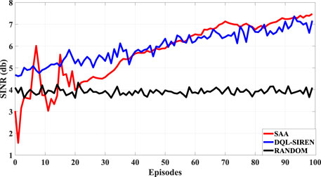
FIGURE 4. Comparison of the SAA, the DQL-SIREN and the Random policy.
We generate 3,000 = 100, ×, 30 instances of the source-relay and relay destination channels for the whole grid (20, ×, 20). Every 30 time steps we initialize the relays to random positions in the grid and let them move. We plot the average SINR for every 30 steps of the algorithms.
5.3 Simulation Results and Discussion
We present the results of our simulations in Figure 4. As we stated before, the results correspond to the average SINR at the destination for 100 episodes. Each episode consists of 30 time steps. The runs correspond to the average over six different seeds.
We compare three different policies. The first one is the Random policy, where each relay chooses the displacement for the next step at random. The second policy is the DQL-SIREN that solves the dynamic program (maximization of the discounted sum of VIs for every relay from the current time step to the infinite horizon). The third policy is the myopic SAA that corresponds to the stochastic program and optimizes each individual relay’s VI for the subsequent slot.
As one can see that both the SAA and the DQL-SIREN perform significantly better than the Random policy (they both achieve an average SINR of approximately 7 db in contrast to the Random policy that achieves about 4 db). Table 1 contains a head-to-head comparison of the SAA and the DQL-SIREN approaches regarding some qualitative and some quantitative features.
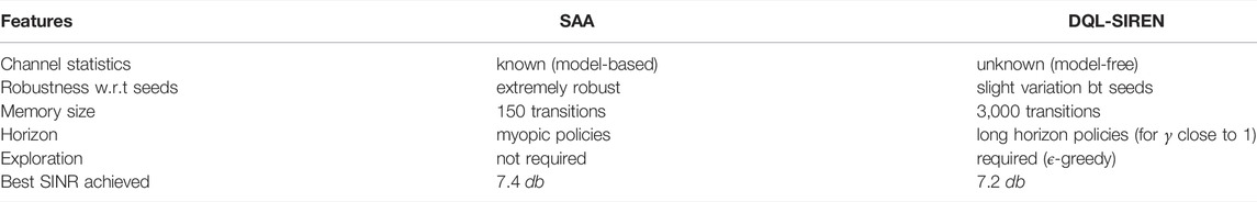
TABLE 1. Table of comparison between the two methods regarding key features.
The convergence of the DQL-SIREN is faster than that of SAA. This is reasonable since, when it comes to the SAA approach, for the first five episodes there have not been collected enough samples (150). Both SAA and DQL-SIREN perform approximately the same in terms of average SINR. Towards the end of the experiments there is a small gap between the two (with the SAA performing slightly better). This can be attributed to the ϵ-greedy policy of the DQL-SIREN, where ϵ never goes to zero (choosing a random action a small percentage of the time for maintaining exploration).
There are some interesting inferences that one can make, based on the simulations. First of all, even though the SAA is myopic and only attempts to maximize the SINR for the subsequent time slot, works quite well in the sense of the aggregated statistic of the average SINR. This is a clear indication that, for the formulated problem, being greedy translates to performing adequately in the sense of cumulative reward.
Of course this peculiarity stands true only when the statistics of the channels are completely known and do not change significantly during the operation time. Apparently, in such a scenario, the phenomenon of delayed rewards is not much prevalent.
6 Conclusion
In this paper, we examine the discrete motion control for mobile relays facilitating the communication between a source and a destination. We compare two different approaches to tackle the problem. The first approach employs stochastic programming for scheduling the relay motion. This approach is myopic meaning that it seeks to maximize the SINR at the destination, only at the subsequent time slot. In addition, the stochastic programming approach makes specific assumption for the statistics of the channel evolution. The second approach is a deep reinforcement learning approach that is not myopic meaning that its goal is to maximize the discounted sum of SINR at the destination from the subsequent slot to an infinite time horizon. Additionally, the second approach makes no particular assumptions for the channel statistics. We test our methods in synthetic channel data produced in accordance to a known model for spatiotemporally varying channels. Both methods perform similarly and achieve significant improvement in comparison to a standard random policy for relay motion. We also provide a head-to-head comparison of the two approaches regarding various key qualitative and quantitative features. As future work, we plan on extending the current methods for scenarios with multiple source-destination communication pairs and, possibly, include the existence of eavesdroppers.
Data Availability Statement
The raw data supporting the conclusion of this article will be made available by the authors, without undue reservation.
Author Contributions
All authors listed have made a substantial, direct, and intellectual contribution to the work and approved it for publication.
Funding
Work supported by ARO under grant W911NF2110071.
Conflict of Interest
The authors declare that the research was conducted in the absence of any commercial or financial relationships that could be construed as a potential conflict of interest.
Publisher’s Note
All claims expressed in this article are solely those of the authors and do not necessarily represent those of their affiliated organizations, or those of the publisher, the editors and the reviewers. Any product that may be evaluated in this article, or claim that may be made by its manufacturer, is not guaranteed or endorsed by the publisher.
References
Barriac, G., Mudumbai, R., and Madhow, U. (2004). “Distributed Beamforming for Information Transfer in Sensor Networks,” in Third International Symposium on Information Processing in Sensor Networks, 2004 (IEEE), 81–88. doi:10.1145/984622.984635
Bertsekas, D. (1995). Dynamic Programming & Optimal Control. 4th edn., II. Belmont, Massachusetts: Athena Scientific.
Bertsekas, D. P., and Shreve, S. E. (1978). Stochastic Optimal Control: The Discrete Time Case, 23. New York: Academic Press.
Cao, Y., Fang, Z., Wu, Y., Zhou, D.-X., and Gu, Q. (2019). Towards Understanding the Spectral Bias of Deep Learning. arXiv preprint arXiv:1912.01198.
Chatzipanagiotis, N., Liu, Y., Petropulu, A., and Zavlanos, M. M. (2014). Distributed Cooperative Beamforming in Multi-Source Multi-Destination Clustered Systems. IEEE Trans. Signal Process. 62, 6105–6117. doi:10.1109/tsp.2014.2359634
Evmorfos, S., Diamantaras, K., and Petropulu, A. (2021a). “Deep Q Learning with Fourier Feature Mapping for Mobile Relay Beamforming Networks,” in 2021 IEEE 22nd International Workshop on Signal Processing Advances in Wireless Communications (SPAWC), 126–130. doi:10.1109/SPAWC51858.2021.9593138
Evmorfos, S., Diamantaras, K., and Petropulu, A. (2021b). “Double Deep Q Learning with Gradient Biasing for Mobile Relay Beamforming Networks,” in 2021 55th Asilomar Conference on Signals, Systems, and Computers, 742–746. doi:10.1109/ieeeconf53345.2021.9723405
Evmorfos, S., Diamantaras, K., and Petropulu, A. (2022). Reinforcement Learning for Motion Policies in Mobile Relaying Networks. IEEE Trans. Signal Process. 70, 850–861. doi:10.1109/TSP.2022.3141305
Gao, F., Cui, T., and Nallanathan, A. (2008). On Channel Estimation and Optimal Training Design for Amplify and Forward Relay Networks. IEEE Trans. Wirel. Commun. 7, 1907–1916. doi:10.1109/TWC.2008.070118
Havary-Nassab, V., Shahbazpanahi, S., Grami, A., and Zhi-Quan Luo, Z.-Q. (2008a). Distributed Beamforming for Relay Networks Based on Second-Order Statistics of the Channel State Information. IEEE Trans. Signal Process. 56, 4306–4316. doi:10.1109/tsp.2008.925945
Havary-Nassab, V., ShahbazPanahi, S., Grami, A., and Zhi-Quan Luo, Z.-Q. (2008b). Distributed Beamforming for Relay Networks Based on Second-Order Statistics of the Channel State Information. IEEE Trans. Signal Process. 56, 4306–4316. doi:10.1109/TSP.2008.925945
Heath, R. W. (2017). Introduction to Wireless Digital Communication: A Signal Processing Perspective. Prentice-Hall.
Jacot, A., Gabriel, F., and Hongler, C. (2018). “Neural Tangent Kernel: Convergence and Generalization in Neural Networks,” in Advances in Neural Information Processing Systems. Editors S. Bengio, H. Wallach, H. Larochelle, K. Grauman, N. Cesa-Bianchi, and R. Garnett (Curran Associates, Inc).31.
Kalogerias, D. S., Chatzipanagiotis, N., Zavlanos, M. M., and Petropulu, A. P. (2013). “Mobile Jammers for Secrecy Rate Maximization in Cooperative Networks,” in Acoustics, Speech and Signal Processing (ICASSP), 2013 IEEE International Conference, 2901–2905. doi:10.1109/ICASSP.2013.6638188
Kalogerias, D. S., and Petropulu, A. P. (2016). “Mobile Beamforming Amp; Spatially Controlled Relay Communications,” in 2016 IEEE International Conference on Acoustics, Speech and Signal Processing (ICASSP), 6405–6409. doi:10.1109/ICASSP.2016
Kalogerias, D. S., and Petropulu, A. P. (2017). Spatially Controlled Relay Beamforming: 2-stage Optimal Policies. Arxiv.
Kalogerias, D. S., and Petropulu, A. P. (2018). Spatially Controlled Relay Beamforming. IEEE Trans. Signal Process. 66, 6418–6433. doi:10.1109/tsp.2018.2875896
Li, J., Petropulu, A. P., and Poor, H. V. (2011). Cooperative Transmission for Relay Networks Based on Second-Order Statistics of Channel State Information. IEEE Trans. Signal Process. 59, 1280–1291. doi:10.1109/TSP.2010.2094614
Liu, Y., and Petropulu, A. P. (2011). On the Sumrate of Amplify-And-Forward Relay Networks with Multiple Source-Destination Pairs. IEEE Trans. Wirel. Commun. 10, 3732–3742. doi:10.1109/twc.2011.091411.101523
MacCartney, G. R., Zhang, J., Nie, S., and Rappaport, T. S. (2013). Path Loss Models for 5G Millimeter Wave Propagation Channels in Urban Microcells. Globecom, 3948–3953. doi:10.1109/glocom.2013.6831690
Mnih, V., Kavukcuoglu, K., Silver, D., Rusu, A. A., Veness, J., Bellemare, M. G., et al. (2015). Human-level Control through Deep Reinforcement Learning. nature 518, 529–533. doi:10.1038/nature14236
Muralidharan, A., and Mostofi, Y. (2017). “First Passage Distance to Connectivity for Mobile Robots,” in Proceedings of the American Control Conference (IEEE), 1517–1523. doi:10.23919/ACC.2017.7963168
Rockafellar, R. T., and Wets, R. J.-B. (2004). Variational Analysis, 317. Springer Science & Business Media.
Shapiro, A., Dentcheva, D., and Ruszczyński, A. (2009). Lectures on Stochastic Programming. 2nd edn. Society for Industrial and Applied Mathematics.
Sitzmann, V., Martel, J., Bergman, A., Lindell, D., and Wetzstein, G. (2020). Implicit Neural Representations with Periodic Activation Functions. Adv. Neural Inf. Process. Syst. 33, 7462–7473.
Yan, Y., and Mostofi, Y. (2013). Co-optimization of Communication and Motion Planning of a Robotic Operation under Resource Constraints and in Fading Environments. IEEE Trans. Wirel. Commun. 12, 1562–1572. doi:10.1109/twc.2013.021213.120138
Yan, Y., and Mostofi, Y. (2012). Robotic Router Formation in Realistic Communication Environments. IEEE Trans. Robot. 28, 810–827. doi:10.1109/TRO.2012.2188163
Keywords: relay networks, discrete motion control, stochastic programming, dynamic programming, deep reinforcement learning
Citation: Evmorfos S, Kalogerias D and Petropulu A (2022) Adaptive Discrete Motion Control for Mobile Relay Networks. Front. Sig. Proc. 2:867388. doi: 10.3389/frsip.2022.867388
Received: 01 February 2022; Accepted: 01 June 2022;
Published: 06 July 2022.
Edited by:
Monica Bugallo, Stony Brook University, United StatesReviewed by:
Francesco Palmieri, University of Campania Luigi Vanvitelli, ItalyStefania Colonnese, Sapienza University of Rome, Italy
Copyright © 2022 Evmorfos, Kalogerias and Petropulu. This is an open-access article distributed under the terms of the Creative Commons Attribution License (CC BY). The use, distribution or reproduction in other forums is permitted, provided the original author(s) and the copyright owner(s) are credited and that the original publication in this journal is cited, in accordance with accepted academic practice. No use, distribution or reproduction is permitted which does not comply with these terms.
*Correspondence: Athina Petropulu, YXRoaW5hcEBydXRnZXJzLmVkdQ==
†These authors have contributed equally to this work